A 2-D process-based model for suspended sediment dynamics:
a first step towards ecological modeling
F. M. Achete1, M. van der Wegen1,2, D. Roelvink1,2,3, and B. Jaffe4 1UNESCO-IHE, Delft, the Netherlands
2Deltares, Delft, the Netherlands
3Delft University of Technology, Delft, the Netherlands
4US Geological Survey Pacific Science Center, Santa Cruz, California, USA Correspondence to: F. M. Achete ([email protected])
Received: 20 December 2014 – Published in Hydrol. Earth Syst. Sci. Discuss.: 02 February 2015 Revised: 29 May 2015 – Accepted: 01 June 2015 – Published: 19 June 2015
Abstract. In estuaries suspended sediment concentration (SSC) is one of the most important contributors to turbid-ity, which influences habitat conditions and ecological func-tions of the system. Sediment dynamics differs depending on sediment supply and hydrodynamic forcing conditions that vary over space and over time. A robust sediment transport model is a first step in developing a chain of models enabling simulations of contaminants, phytoplankton and habitat con-ditions.
This works aims to determine turbidity levels in the complex-geometry delta of the San Francisco estuary using a process-based approach (Delft3D Flexible Mesh software). Our approach includes a detailed calibration against mea-sured SSC levels, a sensitivity analysis on model parameters and the determination of a yearly sediment budget as well as an assessment of model results in terms of turbidity levels for a single year, water year (WY) 2011.
Model results show that our process-based approach is a valuable tool in assessing sediment dynamics and their re-lated ecological parameters over a range of spatial and tem-poral scales. The model may act as the base model for a chain of ecological models assessing the impact of climate change and management scenarios. Here we present a modeling ap-proach that, with limited data, produces reliable predictions and can be useful for estuaries without a large amount of pro-cesses data.
1 Introduction
Rivers transport water and sediments to estuaries and oceans. Sediment dynamics will differ depending on sediment supply and hydrodynamic forcing conditions, both of which vary over space and time. The human impact on sediment pro-duction dates from 3000 years ago, and has been accelerat-ing over the past 1000 years due to considerable engineer-ing works (Syvitski and Kettner, 2011). Milliman and Syvit-ski (1992) estimated that the budget of sediment delivered to the coastal zone varies between 9.3 and 58 Gt per year. Esti-mating the world sediment budget is still a challenge because of the lack of data and detailed modeling studies (Vörös-marty et al., 2003). In addition, there is considerable un-certainty in hydraulic forcing conditions and sediment sup-ply dynamics due to variable adaptation timescales over sea-sons and years (such as varying precipitation and river flow), decades (such as engineering works) and centuries to millen-nia (sea level rise and climate change).
con-tinuous change in sediment dynamics and hence sediment budget in the estuary, and (b) change in sediment availability leading to change in turbidity levels.
Turbidity is a measurement of light attenuation in water and is a key ecological parameter. Fine sediment is the main contributor to turbidity. Therefore, suspended sediment con-centration (SSC) can be translated into turbidity by applying empirical formulations. Besides SSC, algae, plankton, mi-crobes and other substances may also contribute to turbid-ity levels (ASTM International, 2002). High turbidturbid-ity lev-els limit photosynthesis activity by phytoplankton and mi-croalgae, therefore decreasing associated primary production (Cole et al., 1986). Turbidity levels also define habitat condi-tions for endemic species (Davidson-Arnott et al., 2002). For example, in the San Francisco Bay–Delta estuary the delta smelt seeks regions where the turbidity is between 12 and 18 NTU to hide from predators (Baskerville and Lindberg, 2004; Brown et al., 2013). Examples of other ecological im-pacts related to SSC are vegetation stabilization (Morris et al., 2002; Whitcraft and Levin, 2007), and salt marsh survival under sea level rise scenarios (Kirwan et al., 2010; Reed, 2002).
To assess the aforementioned issues, the goal of this work is to provide a detailed analysis of sediment dynam-ics including (a) SSC levels in the Sacramento–San Joaquin delta (Delta), (b) sediment budget and (c) translation of SSC to turbidity levels using a two-dimensional horizon-tal, averaged in the vertical (2DH), process-based, numer-ical model. The 2DH model solves the 2-D vertnumer-ically in-tegrated shallow-water equations coupled with advective– diffusive transport. This process-based model will be able to quantify high-resolution sediment budgets and SSC, both in time (∼monthly/yearly) and space (∼10–100 s of meters). We selected the Delta area as a case study, since the area has been well monitored so that detailed model validation can take place, it hosts endemic species, and allow us to use a 2DH model approach.
The Delta and Bay are covered by a large survey net-work with freely available data on river stage, discharge and SSC and other parameters from the US Geological Survey (USGS) (nwis.waterdata.usgs.gov), Californian De-partment of Water Resources (http://cdec.water.ca.gov/) and National Oceanic and Atmospheric Administration (http:// tidesandcurrents.noaa.gov/). The continuous SSC measure-ment stations are periodically calibrated using water col-lected in situ, that is filtered and weighed in the labora-tory. In addition, the Bay–Delta system has high-resolution (10 m) bathymetry available for all the channels and bays (http://www.d3d-baydelta.org/).
Regarding ecological value, starting from the bottom of the food web, the Delta is the most important area for pri-mary production in the San Francisco estuary. The Delta is 1 order of magnitude more productive than the rest of the es-tuary (Jassby et al., 2002; Kimmerer, 2004). It is an area for spawning, breeding and feeding for many endemic species of
fishes and invertebrates, including some endangered species like delta smelt (Brown et al., 2013), chinook salmon, spring run salmon and steelhead. Additionally, several projects for marsh restoration in the Delta are planned and the success of these projects depends on sediment availability (Brown, 2003).
SSC spatial distribution and temporal variability is impor-tant information for the ecology of estuaries. However, ob-servations including both high spatial and temporal resolu-tion of SSC are difficult to make, so we revert to using cou-pled hydrodynamic–sediment transport models to make pre-dictions at any place and time.
For the first time, a detailed, process-based model is de-veloped for the San Francisco Bay–Delta, to focus on the complex delta sediment dynamics. From this model it is pos-sible to describe the spatial sediment (turbidity) distribution and deposition patterns that are important indicators to as-sess habitat conditions. Seasonal and yearly variations in sed-iment dynamics and turbidity levels can be used as indicators for ecological modeling (Janauer, 2000). This work fills the gap between the physical aspects (hydrodynamic and sedi-ment modeling) and ecology modeling. Previous work fo-cused on understanding the San Francisco Bay–delta system through data analysis (Barnard et al., 2013; Manning and Schoellhamer, 2013; McKee et al., 2006, 2013; Morgan-King and Schoellhamer, 2013; Schoellhamer, 2002, 2011; Wright and Schoellhamer, 2004, 2005), while similar work in other estuaries around the world does not provide a direct link to ecology (Manh et al., 2014).
2 Study area and model
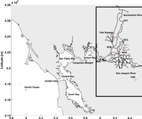
San Francisco estuary is the largest estuary on the US west coast. The estuary comprises San Francisco Bay and the inland Sacramento–San Joaquin Delta (Bay–Delta system), which together cover a total area of 2900 km2 with a mean water depth of 4.6 m (Jassby et al., 1993). The system has a complex geometry consisting of interconnected sub-embayments, channels, rivers, intertidal flats and marshes (Fig. 1). The Sacramento–San Joaquin Delta (Delta) is a col-lection of natural and man-made channel networks and lev-eed islands, where the Sacramento River and the San Joaquin River are the main tributaries followed by Mokelumne River (Delta Atlas, 1995). San Francisco Bay has four sub-embayments. The most landward is Suisun Bay followed by San Pablo Bay, central bay (connecting with the sea through Golden Gate) and, further southward, South Bay.
lo-black rectangle; Fig. 1). The topography greatly influences the wind climate in the Bay–Delta system. Wind velocities are strongest during spring and summer with afternoon north-westerly gusts of about 9 m s−1(Hayes et al., 1984).
San Francisco estuary collects 40 % of the total Califor-nian fresh water discharge. It has a Mediterranean climate, with 70 % of rainfall concentrated between October and April (winter) decreasing until the driest month, September (summer) (Conomos et al., 1985). The orographic lift of the Pacific moist air linked to the winter storms and the snowmelt in early spring govern this wet (winter) and dry (summer) season variability. This system leads to a local hydrological water year (WY) defined as 1 October to 30 September, in-cluding a full wet season in 1 WY.
The Sacramento and San Joaquin rivers, together, account for 90 % of the total fresh water discharge to the estuary (Kimmerer, 2004). The daily inflow to the Delta follows the rain and snowmelt seasonality, with average dry summer dis-charges of 50–150 m3s−1 and wet spring/winter peak dis-charges of 800–2500 m3s−1. The seasonality and geographic distribution of flows leads to several water issues related to agricultural use, habitat maintenance and water export. On a yearly average 300 m3s−1of water is pumped from the South Delta to southern California. The pumping rate is designed to keep the 2 psu (salinity) line landwards of Chipps Island avoiding salinity intrusion in the Delta, allowing for a 2DH modeling approach.
The hydrological cycle in the Bay–Delta determines the sediment input to the system, and thus biota behavior. Mc-Kee et al. (2006) and Ganju and Schoellhamer (2006) ob-served that a large volume of sediment passes through the Delta and arrives to the bay in pulses. They estimated that in 1 day approximately 10 % of the total annual sediment volume could be delivered and in extremely wet years up to 40 % of the annual total sediment volume can be delivered in 7 days. During wet months more than 90 % of the total annual sediment inflow is supplied to the Delta.
The Delta’s recent history is dominated by anthropogenic impacts. In the 1850s hydraulic mining started after placer mining in rivers became unproductive. Hydraulic mining re-mobilized a huge amount of sediment upstream of Sacra-mento. By the end of the nineteenth century the hydraulic mining was outlawed leaving approximately 1.1×10⁹m3of remobilized sediment, which filled mud flats and marshes up to 1 m in the Delta and bay (Wright and Schoellhamer, 2004; Jaffe et al., 2007). At the same time mining prohibi-tion ended, civil works such as dredging and construcprohibi-tion of levees and dams started, reducing the sediment supply to the Delta (Delta Atlas, 1995; Whipple et al., 2012).
Typical SSC in the Delta ranges from 10 to 50 mg L−1, except during high river discharge when SSC can exceed 200 mg L−1 reaching values over 1000 mg L−1 (McKee et al., 2006; Wright and Schoellhamer, 2005). Sediment
bud-and outflow, estimated that about two-thirds of the sediment entering the system is deposited in the Delta (Schoellhamer et al., 2012; Wright and Schoellhamer, 2005). The remain-ing third is exported to the bay, and represents on average 50 % of the total bay sediment supply (McKee et al., 2006), the other half comes from smaller watersheds around the bay (McKee et al., 2013).
Several studies have been carried out to determine sedi-ment pathways and to estimate sedisedi-ment budgets in the Delta area (Schoellhamer et al., 2012; Jaffe et al., 2007; Gilbert, 1917; McKee et al., 2006, 2013; Wright and Schoellhamer, 2005). These studies were based on data analysis and con-ceptual hindcast models. Although the region has a unique network of surveying stations, there are many channels with-out measuring stations. This might lead to incomplete system understanding and knowledge deficits for the development of water and ecosystem management plans. The monitoring stations are located in discrete points hampering spatial anal-ysis. Also, the impact of future scenarios related to climate change (i.e., sea level rise and changing hydrographs) or dif-ferent pumping strategies remains uncertain.
2.1 Model description
Structured grid models such as Delft3D and ROMS (Re-gional Oceanic Modeling System) have been widely used and accepted in estuarine hydrodynamics and morphody-namics modeling including studies of the San Francisco estu-ary (Ganju and Schoellhamer, 2009; Ganju et al., 2009; van der Wegen et al., 2011). In all of these studies the Delta was schematized as two long channels because the grid is not flexible, which would have allowed for efficient 2-D mod-eling of the rivers, channels and flooded island of the system together with the bay.
In cases with complex geometry, unstructured grids or a finite volume model is more suitable. There are three widely known unstructured grid models: (1) the TELEMAC-MASCARET (Hervouet, 2007), (2) the Unstruc-tured Tidal, residual, intertidal mudflat model (UnTRIM) (Casulli and Walters, 2000; Bever and MacWilliams, 2013) and (3) Delft3D Flexible Mesh (D3D FM) (Kernkamp et al., 2010). The first two models are purely triangle based and are not directly coupled (yet) with sediment transport and/or wa-ter quality and ecology models.
Figure 1. Location of the San Francisco Bay–Delta. The black
rect-angle highlights the Delta, and the red squares indicate measure-ment stations.
in terms of triangles, (curvilinear) quadrilaterals, pentagons and hexagons, or any combination of these shapes. Orthogo-nal quadrilaterals are the most computatioOrthogo-nally efficient cells and are used whenever the geometry allows. Kernkamp et al. (2010) and the D3D FM manual (Deltares, 2014) describe in detail the grid aspects and numerical solvers.
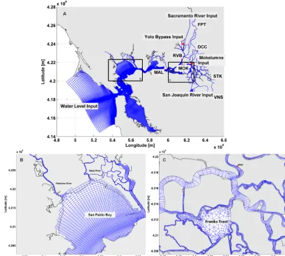
The bay area and river channels are defined by consecu-tive curvilinear grids (quadrilateral) of different resolution. Rivers discharging in the bay, and channel junctions are con-nected by triangles (Fig. 2). The average cell size ranges from 1200 m×1200 m in the coastal area, to 450 m×600 m in the bay area, down to 25×25 m in Delta channels. In the Delta, each channel is represented by at least 3 cells in the across-channel direction (Fig. 2). The grid flexibility allows for including the entire Bay–Delta in a single grid contain-ing 63 844 cells of which about 80 % are rectangles which keeps the computer run times at an acceptable level. It takes 6 real days to run 1 year of hydrodynamics simulation and 12 h to run the sediment module on an 8-core desktop com-puter. Besides the triangular grid orthogonality issues, using an entirely triangular grid for a 1-year simulation would in-crease run times from∼72 to∼192 h.
We assume that the main flow dynamics in the Delta is 2-D, which does not account for vertical stratification. The Delta does not experience salt–fresh water interactions due to the pumping operations and we assume that temperature differences between the top and bottom of the water column do not govern flow characteristics. D3D FM generates hy-drodynamic output for off-line coupling with water quality model DELWAQ (Deltares, 2014). Off-line coupling enables faster calibration and sensitivity analysis. D3D FM generates time series of the following variables: cell link area;
bound-ary definition; water flow through cell link; pointers that give information about neighbors’ cells; cell surface area; cell vol-ume; and shear stress file, which is parameterized in D3D FM using Manning’s coefficient. Given a network of water levels and flow velocities (varying over time) DELWAQ can solve the advection–diffusion–reaction equation for a wide range of substances including fine sediment, the focus of this study. DELWAQ solves sediment source and sink terms by applying the Krone–Parteniades formulation for cohesive sediment transport (Krone, 1962; Ariathurai and Arulanan-dan, 1978) (Eqs. 1 and 2).
D=ws·c·
1−τb τd
,which is approximated as
D=ws·c, (1)
where D is the deposition flux of suspended matter (mg m−2s−1),ws is the settling velocity of suspended mat-ter (m s−1),cis the concentration of suspended matter near the bed (mg m−3),τbis bottom shear stress (Pa) andτdis the critical shear stress for deposition (Pa). The approximation is made assuming, like Winterwerp et al. (2006), that deposi-tion takes place regardless of the prevailing bed shear stress. τdis thus considered much larger thanτband the second term in parentheses of Eq. (1) is small and can be neglected. E=M·(τb/τe−1)forτb> τe (2) whereEis the erosion rate (mg m−2s−1),Mis the first-order erosion rate (mg m−2s−1), andτeis the critical shear stress for erosion (Pa).
2.2 Initial and boundary conditions
The Bay–Delta is a well-measured system; therefore, all the input data to the model are in situ data. Initial bathymetry has 10 m grid resolution, which is based on an ear-lier grid (Foxgrover et al., 2012, http://sfbay.wr.usgs.gov/ sediment/delta/), modified to include new data by Wang and Ateljevich (http://baydeltaoffice.water.ca.gov/modeling/ deltamodeling/modelingdata/DEM.cfm) and further refined. The bathymetry is based on different data sources includ-ing bathymetric soundinclud-ings and lidar data. The hydrodynamic model includes real wind, which results from the model de-scribed by Ludwig and Sinton (2000). The wind model spa-tially interpolates hourly data from more than 30 meteorolog-ical stations into regular 1 km grid cells. Levees are included in the model and temporary barriers are inserted to mimic a typical operating schedule as determined by the California Department of Water Resources (http://baydeltaoffice.water. ca.gov/sdb/tbp/web_pg/tempbsch.cfm).
Figure 2. Numerical mesh for the D3D FM model. Red dots indicate the calibration stations (http://san-francisco-bay-delta-model.
unesco-ihe.org/). Detailed box of the computational grid: (b) San Pablo Bay connecting to the Petaluma and Napa rivers, (c) delta chan-nels and Franks Tract.
than 5 m b.m.s.l. (below mean sea level) including intertidal mud flats, and sand at places deeper than 5 m b.m.s.l., which are primarily the channel regions. This implies that the main Delta channels such as, the Sacramento, San Joaquin and Mokelumne are defined as sandy with a few mud patches. DELWAQ does not compute morphological changes or bed load transport.
In this study we applied five open boundaries. Water lev-els at the seaward boundary are based on hourly measure-ments from the Point Reyes station (tidesandcurrents.noaa. gov/). The other four landward boundaries are river discharge boundaries at the Sacramento River (Freeport), Yolo By-pass (YOLO) (upstream water divergence from Sacramento River), San Joaquin River and Mokelumne River. Studies show that Sacramento River accounts for 85 % of the total sediment inflow to the Delta, while the San Joaquin River accounts for 13 % (Wright and Schoellhamer, 2005), so it is reasonable to apply two sediment discharge boundaries at the
Sacramento and San Joaquin rivers. All river boundaries have unidirectional flow and are landward of tidal influence.
The river water flow hourly input data at the FPT, the VNS and YOLO were obtained from the California Data Exchange Center website (cdec.water.ca.gov/) (Fig. 3). The sediment input data, for both input stations FPT and VNS, and cal-ibration stations S Mokelumne R (SMR), N Mokelumne R (NMR), Rio Vista (RVB), Mokelumne (MOK), Little Potato slough (LPS), Middle River (MDM), Stockton (STK) and Mallard Island (MAL) (Fig. 3), were obtained by personal communication from USGS Sacramento; these data are part of a monitoring program (http://sfbay.wr.usgs.gov).
pro-Figure 3. Input boundary conditions. The top panel is water level
at Point Reyes. The lower three panels show discharge in a dashed blue line and SSC in a solid green line for Sacramento River at FPT, San Joaquin River at VNS and Mokelumne River at Woodbridge, respectively.
portional to SSC. To define the rating curve it is necessary to sample water, filter it and weigh the filter. However, in some locations the cloud of points when correlating pho-tocurrent and filtered weight shows a large scatter. Large scatter leads to errors in converting photocurrent to SSC. The causes for errors include variation in particle size, particle de-segregation (cohesiveness, flocculation, organic-rich estuar-ine mud), particle shape effects and sediment-concentration effects (Kineke and Sternberg, 1992; Downing, 2006; Suther-land et al., 2000; Gibbs and Wolanski, 1992; Ludwig and Hanes, 1990). Wright and Schoellhamer (2005) showed that for the Sacramento–San Joaquin delta these errors can sum up to 39 %, when calculating sediment fluxes through Rio Vista.
In this work we modeled the 2011 WY – 1 October 2010 to 30 September 2011. First, we ran D3D FM for this year to calculate water level, velocities, cell volume and shear stresses. Then, the 1 year hydrodynamic results were im-ported in DELWAQ which calculated SSC levels.
The SSC model results are compared to in situ measured SSC data. The calibration process assesses the sensitivity of sediment characteristics such as fall velocity (ws), critical shear stress (τcr) and erosion coefficient (M). The model out-puts are the spatial and temporal distribution of SSC
(turbid-ity), yearly sediment budget for different Delta regions, and the sediment export to the bay.
3 Results
Our focus is to represent realistic SSC levels capturing the peaks, timing and duration, and to develop a sediment bud-get to assess sediment trapping in the Delta (Fig. 1, high-lighted by the black rectangle). Throughout the following sections the results are analyzed in terms of tide-averaged quantities by filtering data and model results to frequencies lower than 2 days. We applied a Butterworth filter with a cut-off frequency of 1/30 h−1as presented in Ganju and Schoell-hamer (2006).
3.1 Calibration
The results shown below are the derived from an extensive calibration process where the different sediment fractions pa-rameters (ws,τcrandM) were tested. The first attempt ap-plied multiple fraction settings presented in previous works (van der Wegen et al., 2011; Ganju and Schoellhamer, 2009). However, tests with a single mud fraction proved to be con-sistent with the data, representative of the sediment budget, and allow for a simpler model setting and better understand-ing of the SSC dynamics. In addition, with a sunderstand-ingle fraction it was possible to reproduce more than 90 % of the sediment budget for the Delta when compared with the sediment bud-get derived from in situ data.
The best fit of the calibration process (uRMS=1 and skill=0.8) for the entire domain was obtained in the standard run, which has ws of 0.25 mm s−1,τcrerosion of 0.25 Pa and Mof 10−4kg m−2s−1. The initial bed sediment availability is defined by one mud (shoals) and one sand (channels) frac-tion. The analysis present below is based in the standard run, and the sensitivity analysis varies the 3 parameters using the standard run as a mid-point.
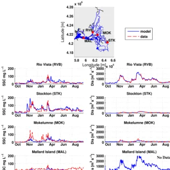
3.2 Suspended sediment dynamics (water year 2011) The 2011 WY simulation reproduces the SSC seasonal varia-tion in the main Delta regions such as the north (Sacramento River) represented by Rio Vista station (RVB), the south (San Joaquin River) represented by Stockton (STK), central-east delta represented by Mokelumne station (MOK) and delta output represented by Mallard Island (MAL) (Fig. 4).
[image:6.612.50.286.65.328.2]Figure 4. Calibration station locations (top panel) and comparison of model outputs and measured data. Left panels show SSC calibration
and right panels the show discharge. Data are dashed red lines and model results are solid blue lines. Note that in the discharge plots of RVB and STK the data line is behind the model line.
The differences found between the model and data are further discussed in Appendix B.
3.3 Sensitivity analysis Sediment fraction analysis
We considered one fraction for simplicity and because it re-produces more than 90 % of the sediment budget throughout the Delta as well as the seasonal variability of SSC levels. Although more mud fractions considerably increase running time, several tests with multiple fractions were done to ex-plore possibilities for improving the model results.
Including heavier fractions changes the peaks timing and also lowers the SSC curve. Comparing the standard run (ws=0.25 mm s−1,T =0.25 Pa, M=10−4kg m−2s−1 and bottom composition with mud available shallower than 5 m) to another run using 15 % of a heavier frac-tion (ws=1.5 mm s−1) and 30 % of a lighter fraction (ws=0.15 mm s−1), showed that the peak magnitudes were
underestimated but the first peak timing is closer to the data and the spurious peak mid-May is lower.
To be able to find a single best parameter setting a sen-sitivity analysis was done varying the main parameters in the Krone–Parteniades formulation (Table 1). Regarding sed-iment flux, these tests show that RVB and MAL are more sen-sitive to parameter change than STK (Fig. 5). The model re-sults are most sensitive to the critical shear stress for erosion and least sensitive to the erosion coefficient. Analyzing the time series, one concludes that in stations where the fluxes are higher, the change in critical shear stress is less impor-tant, since during most of the time the shear stress is already higher than any given critical shear stress.
Table 1. Parameters set of sensitivity analysis.
Parameters Minimum Maximum
Standard w=0.25;τ=0.25;M=1×10⁻⁴ Fall velocity ws (mm s−1) 0.15 0.38
[image:8.612.121.476.375.536.2]Critical shear stressτcr (Pa) 0.125 0.5 Erosion coefficientM (kg m2s−1) 2.5×10⁻⁵ 1×10⁻²
Figure 5. Sensitivity analysis for sediment flux at RVB on the Sacramento River (green squares), at STK on the San Joaquin River (red
triangles) and at MAL where the Delta meets the Bay (blue circles). The colored lines indicate the data values.
Figure 6. Statistical metrics for sensitivity runs. (a) Unbiased root mean square and (b) skill. On thexaxis are the different runs. Colored symbols are stations RVB (green square), STK (red triangle) and MAL (blue circle).
uRMSE= 1
N N X
i=1
Xmi−Xm XOi−XO 2
!0.5
, (3)
whereN is the time series size,Xis the variable to be com-pared, in this case SSC, and X is the time-averaged value. Subscript “m” and “O” represent modeled and observed val-ues, respectively.
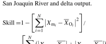
Skill is a single quantitative metric for model performance (Willmott, 1981). When skill equals 1 the model perfectly re-produces the data. The two metrics where evaluated at RVB,
STK and MAL, representing respectively Sacramento River, San Joaquin River and delta output.
Skill=1− " N
X
i=1
Xmi−XOi 2
#
/ " N
X
i−1
Xmi−XO +
XOi−XO 2
#
(4)
[image:8.612.312.485.619.691.2]3.4 Initial bottom composition
To study the importance of initial bottom sediment availabil-ity we considered two cases: one excluding sediment (no sed-iment available at the bed) and the other with mud at places shallower than 5 m b.m.s.l., the same setting as the standard run.
We did some tests varying the 5 m threshold. From 3 to 10 m the final results are all similar. However, allowing mud availability in the channels deeper than 10 m starts to affect the SSC levels. Time series of SSC comparing the two cases show that bottom composition has virtually no influence on SSC after the first couple of days. This result also applies for different mud fractions availability and suggests it may be possible to accurately model less-measured estuaries where virtually no bottom sediment data are available.
Another test shows that it is better to initialize the model with no sediment at the bed than with mud available in the en-tire domain. Initializing the channels with loose mud gener-ates unrealistically high SSC levels through the years, which can take up to 5 years to be reworked.
4 Discussion
In the previous section we presented the model calibration, a normal practice in the modeling process. In this section we discuss the new insights that were derived from the model results. Although these insights are specific to the San Fran-cisco Bay–Delta system, the same approach can be applied to other estuaries and deltas. The model produces detailed sediment dynamics and the main paths in which sediment is transported in the Delta. Sediment flux calculations define the sediment dynamics, while gradients in sediment describe the sediment distribution and deposition pattern in the Delta. We also discuss daily and seasonal variation of turbidity lev-els.
4.1 Spatial sediment distribution
We start the analysis by exploring the general Delta be-havior. During dry periods SSC in the entire Delta is low (<20 mg L−1) and the Delta water is relatively clear. The current model results confirm that the Sacramento River is the main sediment supplier into the Delta (Wright and Schoellhamer, 2004; Schoellhamer et al., 2012). The Sacra-mento River peak flow fills the north and partially fills the central/east delta with sediment. However, the rest of the Delta has quite low levels (∼20 mg L−1) of SSC all year long. Passing VNS, the San Joaquin River main branch flows to the east; however, the SSC peak does not reach much fur-ther than STK. The west branch goes toward the water pump-ing stations where the sediment is pumped out of the system.
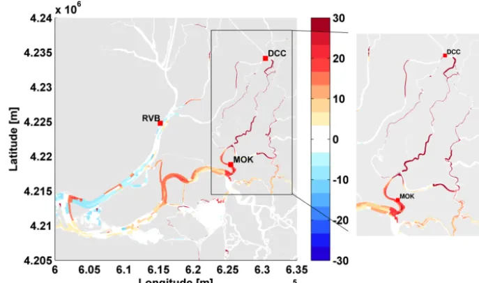
Three Mile slough (TMS) and the delta cross channel (DCC) connect the Sacramento River with the central and eastern Delta. Model results show that together they carry 60 Kt per year of sediment southward. DCC operation con-trols SSC levels in the eastern/central Delta to a large extent. To show the importance of the DCC we run the model twice, once with the DCC always open and once always closed. When the DCC is open, high SSC Sacramento River wa-ter (∼150 mg L−1) flows towards the Mokelumne River and eastern delta increasing the overall SSC in the area. When it is closed SSC levels in the central and eastern Delta are about 30 mg L−1lower than in the previous case (Fig. 7). The ef-fect of opening the DCC can be observed in the SSC level at the San Joaquin River from the MOK station seawards. In the Sacramento River, the opening decreases SSC levels, by about 10 mg L−1and affects the river SSC all the way to Mallard Island (Fig. 7).
During peak river discharge, Sacramento River sediment reaches Mallard Island in approximately 3 days, Carquinez straight in 5 days and the Golden Gate Bridge in approx-imately 10 days. This timing is proportional to river dis-charge. However, from Mallard Island seawards this estimate is inexact due to the 2-D approximation. San Joaquin River sediment remains largely trapped in the southern delta. The flooded islands, breached levees like Franks Tract, present a different behavior. During the entire year the SSC levels are below 15 mg L−1– the river peak discharge signal does not affect them.
Sediment flux is a useful tool for a quantitative and qual-itative analysis of the sediment pathways and its derivative gives sedimentation/erosion patterns. Sediment flux is de-fined by the product of water velocity (U) times cross sec-tional area (A) times SSC (C) (Eq. 5).
Fsed=U·A·C (5)
The yearly sediment flux through FPT from model re-sults is 1132 Kt yr−1 (thousand metric tons per year) and 1096 Kt yr−1from data. Farther seaward on the Sacramento River at RVB the sediment flux is 832 Kt yr−1(994 Kt yr−1, data). Sediment flux at MAL is 617 Kt yr−1 (654 Kt yr−1) (Fig. 8). We calculate that 30 Kt yr−1 of Sacramento River sediment flows to the eastern Delta through the DCC, and 30 Kt yr−1 through TMS and 20 Kt yr−1 from Georgina slough. The San Joaquin River carries 490 Kt yr−1 (498) through VNS, and at STK 205 Kt yr−1(190 Kt yr−1). An esti-mated 100 Kt yr−1is exported through pumping. To close the system in central delta, the flux through Jersey point (JPT) is 126 Kt yr−1(no data) and at the Dutch cross channel (DCH) approximately zero (no data) (Fig. 8).
Figure 7. Anomaly of a SSC (mg L−1) snapshot between runs with open–closed DCC. This pattern is representative in time as well. The right panel is a detailed box between the DCC and MOK (black rectangle). Red shades represent regions where the SSC level is higher in the open than the close scenario, the blue shades where it was lower.
Figure 8. Water discharge (a) and sediment flux (b) pathway models. The arrows represent the water (a) and sediment (b) fluxes through the
cross sections. Area of the arrow is proportional to the flux. Fluxes from data are in red and from the model are in blue. Inside each polygon are the trapping efficiency and deposition volume for the area. The bay portion is dashed because the model is 2-D and 3-D processes occur in that region.
region are inaccurate. Therefore, Fig. 8 shows preliminary sediment flux to the bay by a dashed line.
4.2 Sediment budget
[image:10.612.51.551.323.587.2]and bay in order to define sediment availability for ecology purposes. The model results agree with data estimations that about two-thirds of the sediment input is retained in the Delta (Schoellhamer et al., 2012; Wright and Schoellhamer, 2005), and retention is consistent throughout the years (Cappiella et al., 1999; Jaffe et al., 1998; Wright and Schoellhamer, 2004). Because the D3D FM model provides a detailed description of the sediment pathways, it is possible to further understand and describe the sediment budget in Delta sub-regions (north, central and south) and to compare model results to data when available (M. King, personal communication, 2012).
Besides the overall spatial trend, different parts of the Delta have different trapping efficiencies: the northern Delta (the least efficient) traps∼23 %; central/eastern Delta traps 32 %; central/western 65 %; and the most efficient region, the southern Delta, traps 67 % of the sediment input. The highest trapping efficient regions are where islands inundated through levee breaching (Wright and Schoellhamer, 2005).
Of the total Sacramento River sediment input 40 % stays in the northern Delta and about 40 % is exported to the Bay. The remaining 20 % deposits in the central/eastern delta and only 2 % travels all the way to the south Delta. About 70 % of San Joaquin sediment deposits in the southern Delta, 10 % goes to the central Delta, 15 % is exported via Clifton court pump-ing facilities and 5 % is exported to the bay. This transport is reflected in the bottom composition of the Delta. Sacramento River sediment dominates the northern and central Delta and San Joaquin River sediment dominates the southern delta bottom composition (Fig. 9).
It is enlightening to divide the sediment budget analysis into wet and the dry seasons, since the delta has different dynamics for each season. Water year 2011 was a wet year, with the wet season lasting from mid-January until the end of May. During the wet period 60 % of the yearly sediment in-put budget entered the delta through FPT and VNS and 70 % of the yearly budget was exported through MAL. In the wet season the high river water discharges and SSC pulses flush the entire delta with sediment. In this season high SSC gradi-ents are observed in the plume fronts leading to rapid changes in habitat conditions for many species. After the front the high SSC level can last for more than 1 month, indicating changing in habitat conditions
During the dry season the delta experiences lower river discharges and SSC levels resulting in lower sediment trans-port rates. In the dry season SSC levels do not have peaks and are more uniform. During the dry season the water is clear and the advective flux is lower, which will be discussed in the next section.
4.3 Sediment flux analysis
[image:11.612.322.529.66.282.2]SSC peaks at FPT can be tracked down the estuary. At the RVB station the SSC peak follows the same dynamic as that
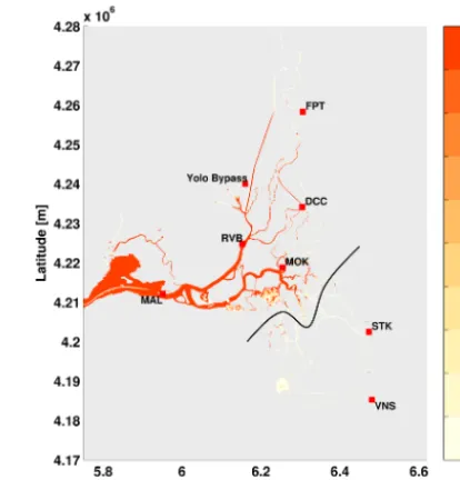
Figure 9. Sediment bottom composition after 1 year, starting with
no bed sediment available. Red shades indicate dominance of Sacra-mento River sediments and white shades dominance of San Joaquin River sediments. The black line highlights where this separation oc-curs.
observed at FPT; however, this behavior does not apply for the entire delta. Schoellhamer and Wright (2005) observed that the river signal is attenuated through the estuary. This attenuation can be understood by analyzing changes in the dominant sediment flux component.
Figure 10. Sediment flux calculations for several stations within the Delta. (a), (c), (e) and (g) show the sediment flux change following the
Figure 11. Modeled deposition in millimeters for 1 year period.
followed by RVB down to Mallard Island where the Delta joins the bay. Stations following the San Joaquin River are VNS, STK and MOK. Three Mile Slough and San Joaquin Junction (SJJ) represent the Delta smaller channels.
Sacramento River at FPT, the most landward station, ex-periences no tidal influence so the flux is purely advective. At RVB, which is seaward, there are tidal fluctuations and the dispersive flux is responsible for 22 % of the total flux; however, no Stokes drift flux is present (Fig. 10). In contrast, Stokes drift accounts for 33 % of the total flux in MAL sta-tion implying that tides have a bigger influence in this region. An analogue can be drawn to the San Joaquin branch, where VNS and STK experience only advective terms. At MOK and SJJ dispersive (20 and 63 %, respectively) and Stokes flux (5 and 11 %) start to influence the total flux (Fig. 10). The analyses of the three different flux components in smaller Delta channels show that river and tidal signals are equally important. The river peak signal is less important in-side smaller channels than in rivers. At TMS, the dispersive flow accounts for 60 % of the total flux.
The flux analyses show that there is no change in the Delta net circulation when comparing wet and dry seasons. There is not a major change in the flux direction when comparing the seasons. However, there is a change in importance of each flux component.
[image:13.612.74.263.66.272.2]Figure 10 shows that dispersive flux and Stokes drift rel-ative contributions vary seasonally. When river discharge is high the relative contribution of dispersive flux is lower than during low flow conditions. This pattern is more apparent at stations where the river signal is stronger. At RVB the dis-persive flux contribution is about 15 % during the wet season and 26 % in the dry season; the same applies for MAL and STK. In smaller channels, like TMS and SJJ, the dispersive flux seasonal variation is milder, varying about 10 %, from
Figure 12. Turbidity in each Delta region. For each region, the left
bars indicates wet season and the right bars the dry season. The light gray bars indicate the mean turbidity over the region, the darker bars the spatial deviation and the lines the daily deviation. Each horizontal line represents 10 NTU.
55 % in the wet season to 65 % in the dry season. In the dry season the change in flux contributions, from advective to dispersive and Stokes drift, leads to a lower net export of sediment from the Delta, even though the concentrations in the Delta are only about 30 mg L−1.
4.4 Sediment deposition pattern
The flux changes from completely advective to dispersive and Stokes drift sheds some light on the Delta deposition areas. The places where the dispersive flux starts to play a role, near RVB and MOK, are the same places where net de-position is observed (Fig. 11). Other locations where consid-erable sedimentation takes place are in flooded island areas, such as Franks Tract and the Clifton court. The 2-D model is sufficient for such areas (Fig. 11).
The San Joaquin River downstream of Stockton experi-ences high deposition. This finding is confirmed by constant dredging needed to maintain the Stockton navigation chan-nel. The river discharge modulates the deposition pattern in the main channels. In the Sacramento deposited sediment is gradually washed away and transported to the mud flats at the channel margins, until the next peak. At the flooded islands the sedimentation process is gradual and steady, erosion is not observed in these areas.
4.5 Turbidity
So far the discussion presented is in terms of SSC levels for the standard run, budgets and fluxes, while ecological analysis is often based on turbidity levels. SSC and turbidity are correlated by rating curves as log10 (SSC)=a·log10 (Turb)+b, where a and b are lo-cal parameters empirilo-cally defined for each Delta area. For the northern areaa=0.85 andb=0.35, central/western area a=0.91 andb=0.29, central/easterna=0.72 andb=0.26, Southern a=1.16 and b=0.27 and Eastern a=0.914 andb=0.29 (USGS Sacramento, personal communication, 2014).
In this section we present average values for turbidity within a specific Delta region as well as its seasonal and daily variations (Fig. 12). Generally, the mean turbidity lev-els and spatial variations are higher during the wet season than during the dry season. During the wet season, the south-ern area had the highest mean value (50 NTU), and deviation (15 NTU), caused by a combination of large sediment supply and low flow velocities. The Northern region is the second most turbid area (45±10 NTU), where sediment transported by the Sacramento River flows in the channels, increasing the turbidity levels. The central-western region is the least turbid area (5±2 NTU) and, as previously shown, it has the highest trapping efficiency of the entire Delta. In the dry season the mean turbidity daily variation decreases in the entire Delta. The opening of the DCC during the dry season lets sediment from the Sacramento River enter these areas, increasing the mean turbidity level. The spatial distribution of the most tur-bid areas is the same as in the wet season. The daily devi-ation is mostly proportional to the turbidity level and to the distance from the sea. In the southern and western areas the daily variation is higher during the dry season. It shows that there is a strong tidal signal in these parts of the Delta.
The DCC and Georgina Slough (GLS) channels that con-nect the Sacramento and San Joaquin rivers are important bridges to export sediment from the Sacramento River to the eastern Delta. The smaller channels of the network play a mi-nor role in the Delta sediment budget because the discharges in these channels are considerably smaller than in the rivers. 4.6 Data input discussion
As a well surveyed area that now has a complex process-based model, the Delta offers the opportunity to test how much data are necessary to develop a reliable sediment model. The model supports high temporal and spatial resolu-tion and includes multiple physical processes such as bottom friction, sedimentation and erosion. The available data allow for calibration and validation of model results.
As presented above, with simple settings of one mud frac-tion and simple bed sediment availability the model is capa-ble of representing the main sediment dynamics processes, the peak timing and duration, and results in a sediment
bud-get. The data necessary for accurate modeling and forecast-ing are fine resolution bathymetry to correctly reproduce hy-drodynamics, SSC and discharge at the inflow and outflow boundaries. It is necessary as well to have one to two stations in the domain in order to properly calibrate the model. The results from the calibrated model using these few data can be extrapolated for the entire domain, allowing for closing the sediment budget for the whole system.
The 2-D model results output is available in high temporal (∼hours) and spatial (∼20 m) resolution, and the modeled water quality parameters can be used in other models or for descriptive purposes. With limited input data we can come to a detailed system description with considerable forecast capacity, expanding the applicability of this work to less-measured estuaries.
5 Conclusions
In this work we make a step towards understanding and sim-ulating sediment dynamics from source to sink in a complex estuary. This work shows that it is possible to reproduce the main system sediment dynamics as well as construct an ac-curate detailed budget for complex areas such as the Delta using a 2-D process-based numerical model coupled with a water quality model.
Overall, the model reproduces the SSC peaks and event timing and duration (wet season) as well as the low concen-tration in dry season throughout the Delta, except at Mal-lard where the water column is stratified due to salt intrusion. Stratification issues are not solved in a 2-D model. For this reason we are working on a 3-D model in order to include the bay area, leading to a unique source to sink model.
The Delta has many observation stations. However, this work shows that substantial sediment is exported trough the pumping stations (100 kt yr−1) at the southern Delta where no data in SSC are available. This sediment export needs fur-ther investigation, since it is possible that it was deposited in the channels before the pumps.
We show that with simple sediment settings of one fraction at the input boundary and a simple distribution of bed sedi-ment availability, it is possible to reproduce seasonal varia-tions as well as construct a yearly sediment budget with more than 90 % accuracy when compared with a data derived bud-get. It also shows that it is extremely important to have dis-charge and SSC measurements at least in the input bound-aries and close to the system output in order to be able to calibrate the model settings applied for hydrodynamics and suspended sediment. This methodology now can be applied in less-measured estuaries.
phyto-to define areas of interest and/or venerable areas phyto-to be study, as well as guide data collecting efforts. The present model opens the possibility for forecast and operational modeling. Forecasting the time frame of high levels of SSC (turbidity) allows for planning of measurements campaigns for ecolo-gists, as well as the possibility of tracking potentially con-taminated sediment and be able to make a contingency plan as well as temporary barriers and pumping operations.
Appendix A: Hydrodynamic calibration
The hydrodynamic calibration was carried out for 3-month high river flow conditions (16 December 1999 to 16 March 2000) and a 3-month period of low river flow con-ditions (16 July 2001 to 16 October 2001). All data are in NAVD88 (vertical datum), UTM 10 (horizontal datum) and GMT (time reference).
Hourly measured water levels at Point Reyes (tidesandcurrents.noaa.gov/) were used as seaward boundary condition. Landward boundary conditions for the Sacra-mento River were obtained from daily measured river flow data at Freeport (FPT) and for the San Joaquin River near Vernalis (VNS) (cdec.water.ca.gov/). The inflow from the Yolo Bypass (YOLO) was approximated by curve fitting data from Qyolo and Qrsac.
Measured data for the bay area were obtained from tidesandcurrents.noaa.gov/, for part of the delta from the Cal-ifornia Data Exchange Centre cdec.water.ca.gov/ and for sta-tions with numbers from direct contact with the Department of Water Resources (DWR).
Calibration was carried out by systematically varying the value of the Manning’s coefficient for different sub-areas of the Bay–Delta system. The calibration data analysis includes (local and time varying) influence of air pressure and wind in the definition of the boundary condition as well as in the calibration data inside the modeling domain. These may ac-count for (part of) the error between measurements and mod-eling results. Also, the NAVD88 reference is not known for all measurement stations, although tidal water fluctuations may be modeled properly. To avoid these problems, a bet-ter method to assess the model performance is to focus on water level amplitude and phasing of the different tidal con-stituents. Boundary conditions, calibration data and model results are thus decomposed by Fourier transformation into tidal components which are then compared. By far, the main tidal constituents at Golden Gate (GGT) are O1, K1, N2, M2 and S2, with M2 being the largest. The model represents their values quite well. The difference in amplitude is 1.3 % for M2, up to 14 % for O1, but the phasing shows a maximum of only 3 % (O1)).
Figure B1. Comparison between SSC levels in RVB station in situ
data (dashed red) and model result (solid blue) and FPT station (dot-ted green).
Appendix B: SSC calibration
All stations clearly reproduce SSC peaks during high river flow periods and lower concentrations during the remainder of the year (apart from MAL during the July–August period). The good representation of the peak timing means that the main delta event is reproduced by the model as well as the periods of delta clearance. These two periods are critical for ecological models, and a good representation generates ro-bust input to ecological models. A closer look at Fig. 4 re-veals differences between model results and data. These dif-ferences are discussed station by station in this Appendix.
At RVB, SSC levels are directly proportional to Sacra-mento River discharge (Fig. B3), and that the model properly represents the water discharge peak intensity and duration. However, in the model, the first peak, which occurs in Oc-tober, remobilizes sediment faster than observed in the data. Analyzing the raw data, it is possible to observe a trend of SSC increase which the model overestimates. A probable ex-planation lies in the initial sediment composition of the bed. Defining the bottom sediment composition does not account for consolidation processes; therefore, the first peak comes after the dry season when the mud in the banks has consoli-dated. In the simulation case, when river discharge increases, it remobilizes non-consolidated bottom/bank sediment caus-ing an earlier peak than in the data. Similar behavior is ob-served at STK in December. Sediment trapped in sub-aquatic vegetation and marshes could be another explanation for the slower increase of the first peak as the model discharges for both stations agree with data (Fig. 4).
Another difference between the data and the model results at RVB is the peak in May (second rectangle, Fig. B1), which is not observed in the data. SSC level at the RVB station is di-rectly proportional to water discharge in FPT (Fig. B3, RVB). The May peak is observed in FPT and so should have been transported towards RVB just as the two preceding peaks.
Figure B2. Water discharge (model) and SSC level (data and
model) in MOK station.
However, the data set does not reproduce this peak. One of the possible explanations is an error in measurements, since it comes after a major event and the equipment might be dam-aged. Other explanations could be a different composition of the suspended sediment properties and/or flocculation.
The model underestimates the first and second SSC peaks at MOK. However, the measured SSC signal is not consistent with the local water discharge signal. First, we checked that modeled water discharge is reproducing the local conditions, where data are available from mid-February onwards. The last peak in Fig. 4 (mid-March) shows that water discharge, in situ and modeled SSC have the same rage of variation. Therefore, the SSC levels are proportional to the local water discharge. Earlier, the January SSC data peak is much higher than the water discharge and the SSC level calculated in the model. The same happens in mid-February when no water discharge peak is observed but there is a peak in the SSC data. Again the peaks in SSC could be caused by an error in the measurements or local, diffuse input of sediment such as from local farm waste water or biological activity remobiliz-ing the substrate.
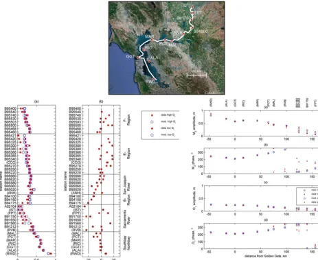
The model represents the wet season SSC peaks well at MAL; however, during the three drier periods of the year the model underestimates SSC levels (Fig. B2). From the scatter plots of water discharge versus SSC (Fig. B3), it is possible to explain the weaker performance of the model during low river flow at MAL. These graphs represent river water dis-charge in FPT lagged by 2 days to SSC in RVB and MAL. Several time lags were tested, as MAL does not have a rea-sonable correlation with any of the time lags; it is presented here with the same time lag as the one for RVB. RVB sta-tion reflects a positive correlasta-tion between river discharge and SSC derived from in situ data and model results. The correlation coefficient (R) at RVB is 0.58.
[image:18.612.325.527.65.204.2]in-Figure B3. Scatter plot discharge versus SSC shown for MAL station on the left-hand (MAL) side and on the right-hand (RVB) side for
RVB station. The red dots represent the data and the blue model results.
[image:19.612.131.463.65.347.2]Acknowledgements. The research is part of the US Geological
Survey Computational Assessment of Scenarios of Change for the Delta Ecosystem (CASCaDE) climate change project (CASCaDE contribution 60). The authors acknowledge the US Geological Survey Priority Ecosystem Studies and California Federation Bay-Delta Program (CALFED) for making this research financially possible. The data used in this work are freely available on the USGS website (nwis.waterdata.usgs.gov). The model applied in this work will be freely available from http://www.d3d-baydelta.org/. We thank Tara Morgan-King, Scott Wright and David Schoellhamer for data collection and analysis. We thank David Schoellhamer for the constructive comments on the manuscript.
Edited by: P. Molnar
References
Ariathurai, R. and Arulanandan, K.: Erosion rates of cohesive soils, J. Hydrol. Eng. Div.-ASCE, 104, 279–283, 1978.
ASTM International: Standards on Disc, Section Eleven, Water and Environmental Technolog, PA, USA, 2002.
Baskerville, B. and Lindberg, C.: The Effect of Light Intensity, Alga Concentration, and Prey Density on the Feeding Behavior of Delta Smelt Larvae, American Fisheries Society Symposium, 219–227, 2004.
Barnard, P. L., Schoellhamer, D. H., Jaffe, B. E., and McKee, L. J.: Sediment transport in the San Francisco Bay coastal system: an overview, Mar. Geol., 345, 3–17, doi:10.1016/j.margeo.2013.04.005, 2013.
Bever, A. J. and MacWilliams, M. L.: Simulating sediment trans-port processes in San Pablo Bay using coupled hydrodynamic, wave, and sediment transport models, Mar. Geol., 345, 235–253, doi:10.1016/j.margeo.2013.06.012, 2013.
Brennan, M. L., Schoellhamer, D. H., Burau, J. R., and Monismith, S. G.: Tidal asymmetry and variability of bed shear stress and sediment bed flux at a site in San Fran-cisco Bay, USA, Environmental Fluid Mechanics Laboratory, Dept. Civil & Environmental Engineering, Stanford University, Stanford, CA, US Geological Survey, Placer Hall, Sacramento, CA, 2002.
Brown, L. R.: A Summary of the San Francisco Tidal Wetlands Restoration Series, San Francisco Estuary and Watershed Sci-ence, San Francisco, 2003.
Brown, L. R., Bennett, W., Wagner, R. W., Morgan-King, T., Knowles, N., Feyrer, F., Schoellhamer, D., Stacey, M., and Dettinger, M.: Implications for future survival of delta smelt from four climate change scenarios for the Sacramento– San Joaquin Delta, California, Estuar. Coast., 36, 754–774, doi:10.1007/s12237-013-9585-4, 2013.
Cappiella, K., Malzone, C., Smith, R., and Jaffe, B. E.: Sedimenta-tion and Bathymetry Changes in Suisun Bay: 1867–1990, USGS, Menlo Park, 1999.
Casulli, V. and Walters, R. A.: An unstructured grid, three-dimensional model based on the shallow water equations, Int. J. Numer. Meth. Fluids, 32, 331–348, doi:10.1002/(sici)1097-0363(20000215)32:3<331::aid-fld941>3.0.co;2-c, 2000.
Cole, B., Cloern, J., and Alpine, A.: Biomass and productivity of three phytoplankton size classes in San Francisco Bay, Estuaries, 9, 117–126, doi:10.2307/1351944, 1986.
Conomos, T. J., Smith, R. E., and Gartner, J. W.: Environmen-tal setting of San Francisco Bay, Hydrobiologia, 129, 1–12, doi:10.1007/BF00048684, 1985.
Davidson-Arnott, R. G. D., van Proosdij, D., Ollerhead, J., and Schostak, L.: Hydrodynamics and sedimentation in salt marshes: examples from a macrotidal marsh, Bay of Fundy, Geomorphol-ogy, 48, 209–231, doi:10.1016/S0169-555X(02)00182-4, 2002. Delta Atlas: Sacramento – San Joaquin Delta Atlas, DWR –
Depart-ment of Water Resources, California, USA, 1995.
Deltares: D-Flow Flexible Mesh, Technical Reference Manual, Deltares, Delft, 82 pp., 2014.
Downing, J.: Twenty-five years with OBS sensors: the good, the bad, and the ugly, Cont. Shelf. Res., 26, 2299–2318, doi:10.1016/j.csr.2006.07.018, 2006.
Dyer, K. R.: The salt balance in stratified estuaries, Estuar. Coast. Mar. Sci., 2, 273–281, doi:10.1016/0302-3524(74)90017-6, 1974.
Foxgrover, A., Smith, R. E., and Jaffe, B. E.: http://sfbay.wr.usgs. gov/sediment/delta/, last access: October 2012.
Ganju, N. K. and Schoellhamer, D. H.: Annual sediment flux es-timates in a tidal strait using surrogate measurements, Estuar. Coast. Shelf S., 69, 165–178, doi:10.1016/j.ecss.2006.04.008, 2006.
Ganju, N. K. and Schoellhamer, D. H.: Calibration of an estuarine sediment transport model to sediment fluxes as an intermediate step for simulation of geomorphic evolution, Cont. Shelf. Res., 29, 148–158, doi:10.1016/j.csr.2007.09.005, 2009.
Ganju, N. K., Schoellhamer, D. H., and Jaffe, B. E.: Hindcast-ing of decadal-timescale estuarine bathymetric change with a tidal-timescale model, J. Geophys. Res., 114, F04019, doi:10.1029/2008jf001191, 2009.
Gibbs, R. J. and Wolanski, E.: The effect of flocs on opti-cal backscattering measurements of suspended material con-centration, Mar. Geol., 107, 289–291, doi:10.1016/0025-3227(92)90078-V, 1992.
Gilbert, G. K.: Hydraulic-Mining Debris in the Sierra Nevada, Pro-fessional Paper 105, USGS, Califronia, USA, 154 pp., 1917. Hayes, T. P., Kinney, J. J., and Wheeler, N. J.: California Surface
Wind Climatology, California Air Resources Board, Aerometric Data Division, California, USA, 107 pp., 1984.
Hervouet, J.-M.: Hydrodynamics of Free Surface Flows, John Wi-ley & Sons, Ltd, 1–360, 2007.
Jaffe, B. E., Smith, R., and Torresan, L.: Sedimentation and Bathy-metric Change in San Pablo Bay: 1856–1983, USGS, Menlo Park, 1998.
Jaffe, B. E., Smith, R. E., and Foxgrover, A. C.: Anthropogenic in-fluence on sedimentation and intertidal mudflat change in San Pablo Bay, California: 1856–1983, Estuar. Coast. Shelf S., 73, 175–187, doi:10.1016/j.ecss.2007.02.017, 2007.
Janauer, G. A.: Ecohydrology: fusing concepts and scales, Ecol. Eng., 16, 9–16, doi:10.1016/S0925-8574(00)00072-0, 2000. Jassby, A. D., Cloern, J. E., and Powell, M. A.: Organic carbon
sources and sinks in San Francisco Bay: variability induced by river flow, Mar. Ecol.-Prog. Ser., 95, 39–54, 1993.
Kernkamp, H. W. J., Van Dam, A., Stelling, G. S., and De Goede, E. D.: Efficient scheme for the shallow water equations on un-structured grids with application to the Continental Shelf, Ocean Dynam., 29, 1175–1188, doi:10.1007/s10236-011-0423-6, 2010. Kimmerer, W.: Open water processes of the San Francisco estuary: from physical forcing to biological responses, San Francisco Es-tuary and Watershed Science, San Francisco, 2 pp., 2004. Kineke, G. C. and Sternberg, R. W.: Measurements of high
concentration suspended sediments using the optical backscat-terance sensor, Mar. Geol., 108, 253–258, doi:10.1016/0025-3227(92)90199-R, 1992.
Kirwan, M. L., Guntenspergen, G. R., D’Alpaos, A., Morris, J. T., Mudd, S. M., and Temmerman, S.: Limits on the adaptability of coastal marshes to rising sea level, Geophys. Res. Lett., 37, L23401, doi:10.1029/2010gl045489, 2010.
Krone, R. B.: Flume Studies of the Transport of Sediment in Estuar-ial Shoaling Processes, University of California, Berkeley, Cali-fornia, 1962.
Ludwig, F. L. and Sinton, D.: Evaluating an objective wind analysis technique with a long 25 record of routinely col-lected data, J. Appl. Meteorol., 39, 335–348, doi:10.1175/1520-0450(2000)039<0335:eaowat>2.0.co;2, 2000.
Ludwig, K. A. and Hanes, D. M.: A laboratory evaluation of optical backscatterance suspended solids sensors exposed to sand-mud mixtures, Mar. Geol., 94, 173–179, doi:10.1016/0025-3227(90)90111-V, 1990.
Manh, N. V., Dung, N. V., Hung, N. N., Merz, B., and Apel, H.: Large-scale suspended sediment transport and sediment deposi-tion in the Mekong Delta, Hydrol. Earth Syst. Sci., 18, 3033– 3053, doi:10.5194/hess-18-3033-2014, 2014.
Manning, A. J. and Schoellhamer, D. H.: Factors controlling floc settling velocity along a longitudinal estuarine transect, Mar. Geol., 345, 266–280, doi:10.1016/j.margeo.2013.06.018, 2013. McKee, L. J., Ganju, N. K., and Schoellhamer, D. H.: Estimates of
suspended sediment entering San Francisco Bay from the Sacra-mento and San Joaquin Delta, San Francisco Bay, California, J. Hydrol., 323, 335–352, doi:10.1016/j.jhydrol.2005.09.006, 2006.
McKee, L. J., Lewicki, M., Schoellhamer, D. H., and Ganju, N. K.: Comparison of sediment supply to San Francisco Bay from wa-tersheds draining the Bay Area and the Central Valley of Califor-nia, Mar. Geol., 345, 47–62, doi:10.1016/j.margeo.2013.03.003, 2013.
Milliman, J. D. and Syvitski, J. P. M.: Geomorphic/tectonic con-trol of sediment discharge to the ocean: the importance of small mountainous rivers, J. Geol., 100, 525–544, doi:10.1086/629606, 1992.
Morgan-King, T. and Schoellhamer, D.: Suspended-sediment flux and retention in a backwater tidal slough complex near the landward boundary of an estuary, Estuar. Coast., 36, 300–318, doi:10.1007/s12237-012-9574-z, 2013.
Morris, J. T., Sundareshwar, P. V., Nietch, C. T., Kjerfve, B., and Cahoon, D. R.: Responses of coastal wetlands to ris-ing sea level, Ecology, 83, 2869–2877, doi:10.1890/0012-9658(2002)083[2869:ROCWTR]2.0.CO;2, 2002.
phology, 48, 233–243, 2002.
Schoellhamer, D. H.: Variability of suspended-sediment concen-tration at tidal to annual time scales in San Francisco Bay, USA, Cont. Shelf. Res., 22, 1857–1866, doi:10.1016/S0278-4343(02)00042-0, 2002.
Schoellhamer, D. H.: Sudden clearing of estuarine waters upon crossing the threshold from transport to supply regulation of sediment transport as an erodible sediment pool is de-pleted: San Francisco Bay, 1999, Estuar. Coast., 34, 885–899, doi:10.1007/s12237-011-9382-x, 2011.
Schoellhamer, D. H., Wright, S. A., and Drexler, J.: A Concep-tual Model of Sedimentation in the Sacramento-San Joaquin Delta, San Francisco Estuary and Watershed Science, http: //escholarship.org/uc/item/2652z8sq (last access: June 2015), 2012.
Sutherland, T. F., Lane, P. M., Amos, C. L., and Downing, J.: The calibration of optical backscatter sensors for suspended sed-iment of varying darkness levels, Mar. Geol., 162, 587–597, doi:10.1016/S0025-3227(99)00080-8, 2000.
Syvitski, J. P. M. and Kettner, A. J.: Sediment flux and the Anthropocene, Philos. T. Roy. Soc. A, 369, 957–975, doi:10.1098/rsta.2010.0329, 2011.
van der Wegen, M., Jaffe, B. E., and Roelvink, J. A.: Process-based, morphodynamic hindcast of decadal deposition patterns in San Pablo Bay, California, 1856–1887, J. Geophys. Res.-Earth, 116, F02008, doi:10.1029/2009jf001614, 2011.
Vörösmarty, C. J., Meybeck, M., Fekete, B., Sharma, K., Green, P., and Syvitski, J. P. M.: Anthropogenic sediment reten-tion: major global impact from registered river impound-ments, Global Planet. Change, 39, 169–190, doi:10.1016/S0921-8181(03)00023-7, 2003.
Whipple, A., Grossinger, R., Rankin, D., Stanford, B., and Askevold, R.: Sacramento–San Joaquin Delta historical ecology investigation: exploring patterns and process, San Francisco Es-tuary Institute – Aquatic Science Center, Richmond, CA, 2012. Whitcraft, C. R. and Levin, L. A.: Regulation of benthic algal and
animal communities by salt marsh plants: impact of shading, Ecology, 88, 904–917, doi:10.1890/05-2074, 2007.
Willmott, C. J.: On the validation of models, Phys. Geogr., 2, 184– 194, doi:10.1080/02723646.1981.10642213, 1981.
Winterwerp, J. C., Manning, A. J., Martens, C., de Mulder, T., and Vanlede, J.: A heuristic formula for turbulence-induced floccula-tion of cohesive sediment, Estuar. Coast. Shelf Sci., 68, 195–207, doi:10.1016/j.ecss.2006.02.003, 2006.
Wright, S. A. and Schoellhamer, D. H.: Trends in the sediment yield of the Sacramento River, California, 1957–2001, San Fran-cisco Estuary and Watershed Science, http://repositories.cdlib. org/jmie/sfews/vol2/iss2/art2 (last access: June 2015), 2004. Wright, S. A. and Schoellhamer, D. H.: Estimating sediment
bud-gets at the interface between rivers and estuaries with application to the Sacramento–San Joaquin River Delta, Water Resour. Res., 41, W09428, doi:10.1029/2004wr003753, 2005.