An analytical model for simulating two dimensional multispecies plume migration

Hydrol. Earth Syst. Sci., 20, 733–753, 2016 www.hydrol-earth-syst-sci.net/20/733/2016/ doi:10.5194/hess-20-733-2016

© Author(s) 2016. CC Attribution 3.0 License.

An analytical model for simulating two-dimensional multispecies

plume migration

Jui-Sheng Chen1, Ching-Ping Liang2, Chen-Wuing Liu3, and Loretta Y. Li4

1_{Graduate Institute of Applied Geology, National Central University, Jhongli, Taoyuan 32001, Taiwan} 2_{Department of Environmental Engineering and Science, Fooyin University, Kaohsiung 83101, Taiwan} 3_{Department of Bioenvironmental Systems Engineering, National Taiwan University, Taipei 10617, Taiwan} 4_{Department of Civil Engineering, University of British Columbia, Vancouver, BC V6T 1Z4, Canada} Correspondence to: Chen-Wuing Liu ([email protected])

Received: 2 July 2015 – Published in Hydrol. Earth Syst. Sci. Discuss.: 1 September 2015 Revised: 27 January 2016 – Accepted: 30 January 2016 – Published: 18 February 2016

Abstract. The two-dimensional advection-dispersion

equa-tions coupled with sequential first-order decay reacequa-tions in-volving arbitrary number of species in groundwater system is considered to predict the two-dimensional plume behav-ior of decaying contaminant such as radionuclide and dis-solved chlorinated solvent. Generalized analytical solutions in compact format are derived through the sequential appli-cation of the Laplace, finite Fourier cosine, and generalized integral transform to reduce the coupled partial differential equation system to a set of linear algebraic equations. The system of algebraic equations is next solved for each species in the transformed domain, and the solutions in the original domain are then obtained through consecutive integral trans-form inversions. Explicit trans-form solutions for a special case are derived using the generalized analytical solutions and are compared with the numerical solutions. The analytical re-sults indicate that the analytical solutions are robust, accurate and useful for simulation or screening tools to assess plume behaviors of decaying contaminants.

1 Introduction

Experimental and theoretical studies have been undertaken to understand the fate and transport of dissolved hazardous sub-stances in subsurface environments because human health is threatened by a wide spectrum of contaminants in ground-water and soil. Analytical models are essential and efficient tools for understanding pollutants behavior in subsurface en-vironments. Several analytical solutions for single-species

transport problems have been reported for simulating the transport of various contaminants (Batu, 1989, 1993, 1996; Chen et al., 2008a, b, 2011; Gao et al., 2010, 2012, 2013; Leij et al., 1991, 1993; Park and Zhan, 2001; Pérez Guerrero and Skaggs, 2010; Pérez Guerrero et al., 2013; van Genuchten and Alves, 1982; Yeh, 1981; Zhan et al., 2009; Ziskind et al., 2011). Transport processes of some contaminants such as ra-dionuclides, dissolved chlorinated solvents and nitrogen gen-erally involve a series of first-order or pseudo first-order se-quential decay chain reactions. During migrations of decay-ing contaminants, mobile and toxic successor products may sequentially form and move downstream with elevated con-centrations. Single-species analytical models do not permit transport behaviors of successor species of these decaying contaminants to be evaluated. Analytical models for multi-species transport equations coupled with first-order sequen-tial decay reactions are useful tools for synchronous deter-mination of the fate and transport of the predecessor and suc-cessor species of decaying contaminants. However, there are few analytical solutions for coupled multispecies transport equations compared to a large body of analytical solutions in the literature pertaining to the single-species advective-dispersive transport subject to a wide spectrum of initial and boundary conditions.

734 J.-S. Chen et al.: An analytical model for simulating two-dimensional multispecies plume migration

1971; Lunn et al., 1996; van Genuchten, 1985; Mieles and Zhan, 2012), decomposition by change-of-variables with the help of existing single-species analytical solutions (Sun and Clement, 1999; Sun et al., 1999a, b), Laplace transform com-bined with decomposition of matrix diagonization (Quezada et al., 2004; Srinivasan and Clememt, 2008a, b), decompo-sition by change-of-variables coupled with generalized inte-gral transform (Pérez Guerrero et al., 2009, 2010), sequential integral transforms in association with algebraic decomposi-tion (Chen et al., 2012a, b).

Multi-dimensional solutions are needed for real world applications, making them more attractive than one-dimensional solutions. Bauer et al. (2001) presented the first set of semi-analytical solutions for one-, two-, and three-dimensional coupled multispecies transport problem with distinct retardation coefficients. Explicit analytical solu-tions were derived by Montas (2003) for multi-dimensional advective-dispersive transport coupled with first-order reac-tions for a three-species transport system with distinct retar-dation coefficients of species. Quezada et al. (2004) extended the Clement (2001) strategy to obtain Laplace-domain solu-tions for an arbitrary decay chain length. Most recently, Su-dicky et al. (2013) presented a set of semi-analytical solu-tions to simulate the three-dimensional multi-species trans-port subject to first-order chain-decay reactions involving up to seven species and four decay levels. Basically, their so-lutions were obtained species by species using recursion re-lations between target species and its predecessor species. For a straight decay chain, they derived solutions for up to four species and no generalized expressions with com-pact formats for any target species were obtained. Note that their solutions were derived for the first-type (Dirichlet) in-let conditions which generally bring about physically im-proper mass conservation and significant errors in predicting the concentration distributions especially for a transport sys-tem with a large longitudinal dispersion coefficient (Barry and Sposito, 1988; Parlange et al., 1992). Moreover, in ad-dition to some special cases, the numerical Laplace trans-forms are required to obtain the original time domain solu-tion. Besides the straight decay chain, the analytical model by Clement (2001) and Sudicky et al. (2013) can account for more complicated decay chain problems such as diverging, converging and branched decay chains.

Based on the aforementioned reviews, this study presents a parsimonious explicit analytical model for two-dimensional multispecies transport coupled by a series of first-order decay reactions involving an arbitrary number of species in ground-water system. The derived analytical solutions have four salient features. First, the third-type (Robin) inlet boundary conditions which satisfy mass conservation are considered. Second, the solution is explicit, thus solution can be easily evaluated without invoking the numerical Laplace inversion. Third, the generalized solutions with parsimonious mathe-matical structures are obtained and valid for any species of a decay chain. The parsimonious mathematical structures of

the generalized solutions are easy to code into a computer program for implementing the solution computations for ar-bitrary target species. Fourth, the derived solutions can ac-count for any decay chain length. The explicit analytical so-lutions have applications for evaluation of concentration dis-tribution of arbitrary target species of the real-world decay-ing contaminants. The developed parsimonious model is ro-bustly verified with three example problems and applied to simulate the multispecies plume migration of dissolved ra-dionuclides and chlorinated solvent.

2 Governing equations and analytical solutions

2.1 Derivation of analytical solutions

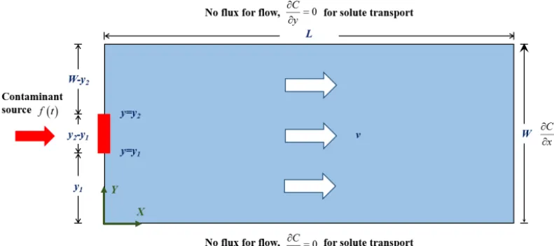
This study considers the problem of decaying contaminant plume migration. The source zone is located in the upstream of groundwater flow. The source zone can represent leaching of radionuclide from a radioactive waste disposal facility or release of chlorinated solvent from the residual NAPL phase into the aqueous phase. After these decaying contaminants enter the aqueous phase, they migrate by one-dimensional advection with flowing groundwater and by simultaneously longitudinal and transverse dispersion processes. While mi-grating in the groundwater system, the contaminants undergo linear isothermal equilibrium sorption and a series of se-quential first-order decaying reactions. Sudicky et al. (2013) provided the detailed modeling scenario. The scenario con-sidered in this study can be ideally described as shown in Fig. 1. A steady and uniform velocity in thex direction is considered in Fig. 1. The governing equations describing two-dimensional reactive transport of the decaying contam-inants and their successor species undergoing linear isother-mal equilibrium sorption and a series of sequential first-order decaying reactions can be mathematically written as

DL

∂2C1(x, y, t )

∂x2 −v

∂C1(x, y, t )

∂x +DT

∂2C1(x, y, t ) ∂y2 −k1R1C1(x, y, t )=R1

∂C1(x, y, t )

∂t (1a)

DL

∂2Ci(x, y, t )

∂x2 −v

∂Ci(x, y, t )

∂x +DT

∂2Ci(x, y, t ) ∂y2

−kiRiCi(x, y, t )+ki−1Ri−1Ci−1(x, y, t )

=Ri

∂Ci(x, y, t )

∂t i=2. . .N. (1b)

whereCi(x, y, t )is the aqueous concentration of species i

[ML−3];x andy are the spatial coordinates in the ground-water flow and perpendicular directions [L], respectively; t is time [T];DLandDTrepresent the longitudinal and trans-verse dispersion coefficients [L2T−1], respectively;vis the average steady and uniform pore-water velocity [LT−1];ki

J.-S. Chen et al.: An analytical model for simulating two-dimensional multispecies plume migration 735

Figure 1. Schematic representation of two-dimensional transport of decaying contaminants in a uniform flow field with flux boundary source

located at of the inlet boundary.

is the retardation coefficient of speciesi[−]. Note that these equations consider that the decay reactions occur simultane-ously in both the aqueous and sorbed phases. If the decay re-actions occur only in the aqueous phase, the retardation coef-ficients in the decay terms in the right-hand sides of Eqs. (1a) and (1b) become unity. For such a case, ki andki−1 in the left-hand sides could be modified as ki

Ri and ki−1

Ri−1 to facilitate

the application of the derived analytical solutions obtained by Eqs. (1a) and (1b).

The initial and boundary conditions for solving Eqs. (1a) and (1b) are

Ci(x, y, t=0)=0 0≤x≤L,0≤y≤W i=1. . .N. (2) −DL

∂Ci(x=0, y, t )

∂x +vCi(x=0, y, t )=vfi(t )

H (y−y1)−H (y−y2)

t≥0 i=1. . .N. (3) ∂Ci(x=L, y, t )

∂x =0,0≤x≤L,0≤y≤W i=1. . .N. (4) ∂Ci(x, y=0, t )

∂y =0t≥0,0≤x≤L i=1. . .N. (5) ∂Ci(x, y=W, t )

∂y =0 t≥0,0≤x≤L i=1. . .N. (6) wherefi(t )is the arbitrary time-dependent source

concen-tration of species i applied at the source segment (H (y− y1)−H (y−y2))at boundary (x=0) which will be specified later [L], H (·)is the Heaviside function,L andW are the length and width of the transport system under consideration [L]. Equation (2) implies that the transport system is free of solute mass at the initial time.

Equation (3) means that a third-type boundary condition satisfying mass conservation at the inlet boundary is con-sidered. Equation (4) considers the concentration gradient to be zero at the exit boundary based on the mass conserva-tion principle. Such a boundary condiconserva-tion has been widely

4

0 20 40 60 80

x [m] 10-12

10-11

10-10

10-9

10-8

10-7

10-6

10-5

10-4

10-3

10-2

10-1

100

R

el

a

ti

v

e

co

n

ce

n

tr

a

ti

o

n

10-12

10-11

10-10

10-9

10-8

10-7

10-6

10-5

10-4

10-3

10-2

10-1

100

0 20 40 60 80

Analytical solution Numerical solution 234U

226_Ra

238Pu

230Th

Fig. 2.

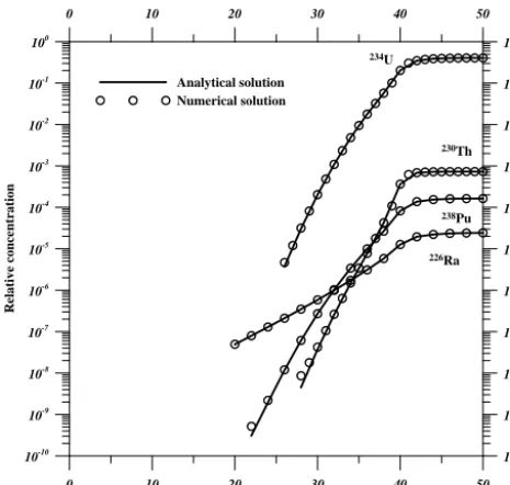
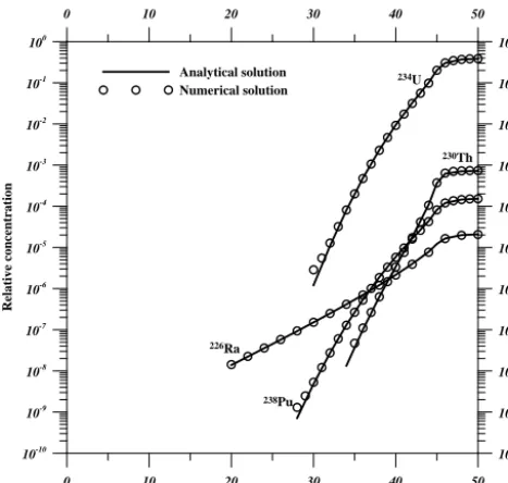
Figure 2. Comparison of spatial concentration profiles of four

species along the longitudinal direction (=50 m) att=1000 years obtained from derived analytical solutions and numerical solutions for convergence test example 1 of four-member radionuclide decay chain238Pu→234U→230Th→226Ra.

bound-736 J.-S. Chen et al.: An analytical model for simulating two-dimensional multispecies plume migration

5

0 10 20 30 40 50

y [m] 10-10 10-9 10-8 10-7 10-6 10-5 10-4 10-3 10-2 10-1 100 R el a ti v e co n ce n tr a ti o n 10-10 10-9 10-8 10-7 10-6 10-5 10-4 10-3 10-2 10-1 100

0 10 20 30 40 50

Analytical solution Numerical solution 234_U 230_Th 238Pu 226_Ra Fig. 3.

Figure 3. Comparison of spatial concentration profiles of four

species along the transverse direction (=0 m) att=1000 years ob-tained from derived analytical solutions and numerical solutions for convergence test example 1 of four-member radionuclide decay chain238Pu→234U→230Th→226Ra.

ary (Barry and Sposito, 1988; Parlange et al., 1992) are used herein. Sudicky et al. (2013) considered the source concen-tration profiles as Gaussian or Heaviside step functions. If Gaussian distributions are desired, we can easily replace the Heaviside function in the right-hand side of Eq. (3) with a Gaussian distribution.

Equations (1)–(6) can be expressed in dimensionless form as

1

P eL

∂2C1(X, Y, Z)

∂X2

−∂C1(X, Y, Z)

∂X + ρ2 P eT

∂2C1(X, Y, Z)

∂Y2

−κC1(X, Y, Z)=R1

∂C1(X, Y, T )

∂T (7a)

1

P eL

∂2_C

i(X, Y, T )

∂X2 −

∂Ci(X, Y, T )

∂X +

ρ2

P eT

∂2_C

i(X, Y, T )

∂Y2 (7b)

−κiCi(X, Y, T )+κi−1Ci−1(X, Y, T )=Ri

∂Ci(X, Y, T )

∂T

i=2. . .N. (7c)

Ci(X, Y, T=0)=0 0≤X≤1,0≤Y≤1 i=1. . .N. (8)

− 1

P eL

∂Ci(X=0, Y, T )

∂X +Ci(X=0, Y, Z)=fi(T ) [H (Y−Y1)−H (Y−Y2)]T ≥0, i=1. . .N. (9) ∂Ci(X=1, Y, T )

∂X =0 T ≥0,0≤Y≤1 i=1. . .N. (10) ∂Ci(X, Y =0, T )

∂Y =0 T≥0,0≤X≤1 i=1. . .N. (11) ∂Ci(X, Y =1, T )

∂Y =0 T≥0,0≤X≤1 i=1. . .N. (12)

Table 1. Transport parameters used for convergence test example 1

involving the four-species radionuclide decay chain problem used by van Genuchten (1985).

Parameter Value

Domain length,L[m] 250

Domain width,W[m] 100

Seepage velocity,v[m year−1] 100

Longitudinal Dispersion coefficient,DL[m2year−1] 1000

Transverse Dispersion coefficient,DT[m2year−1] 100

Retardation coefficient,Ri

238_{Pu 10 000}

234_{U 14 000}

230_{Th 50 000}

226_{Ra 500}

Decay constant,ki[year−1]

238_{Pu 0.0079}

234_{U 0.0000028}

230_{Th 0.0000087}

226_{Ra 0.00043}

Source decay constant,λm[year−1]

238_{Pu 0.0089}

234_{U 0.00100280}

230_{Th 0.00100870}

226_{Ra 0.00143}

where X= x L, Y =

y W, Y1=

y1

W, Y2= y2

W, T = vt

L, P eL= vL

DL, P eT=

vL DT, ρ=

L

W. Our solution strategy used is

ex-tended from the approach proposed by Chen at al. (2012a, b). The core of this approach is that the coupled partial dif-ferential equations are converted into an algebraic equation system via a series of integral transforms and the solutions in the transformed domain for each species are directly and algebraically obtained by sequential substitutions.

Following Chen et al. (2012a, b), the generalized analyti-cal solutions in compact formats can be obtained as follows (with detailed derivation provided in Appendix A)

Ci(X, Y, T )=fi(T )8(n=0)+e P e_L

2 X

∞

X

l=1

K(ξl, X) N (ξl)

pi(ξl, n, T )+qi(ξl, n, T )

8(n=0)2 (ξl) +2

n=∞

X

n=1

(

fi(T )8(n)+e P e_L

2 X

∞

X

l=1

K(ξl, X) N (ξl)

pi(ξl, n, T )+qi(ξl, n, T )8(n)2 (ξl) cos(nπ Y ) (13)

where 8(n)=

Y2−Y1n=0 sin(nπ Y2)−sin(nπ Y1)

nπ n=1,2,3. . .

, ξl is the

J.-S. Chen et al.: An analytical model for simulating two-dimensional multispecies plume migration 737

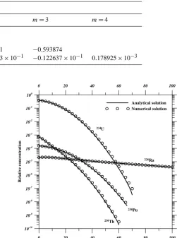
Table 2. Values for coefficients of Bateman-type boundary source for four-species transport problem used by van Genuchten (1985).

Species,i bim

m=1 m=2 m=3 m=4 238_{Pu,i=1 1.25}

234_{U,i=2 −1.25044 1.25044}

230_{Th,i=3 0.443684×10}−3 _{0.593431 −0.593874}

226_{Ra,i=4 −0.516740×10}−6 _0.120853×10−1 _{−0.122637×10}−1 _0.178925×10−3

Figure 4. Comparison of spatial concentration profiles of four

species along the transverse direction (=25 m) at t=1000 years obtained from derived analytical solutions and numerical solutions for convergence test example 1 of four-member radionuclide decay chain238Pu→234U→230Th→226Ra.

ξlcotξl− ξ_l2 P eL +

P eL

4 =0, 2 (ξl)=

P eLξl P e2_L

4 +ξl2

,K(ξl, X)= P eL

2 sin(ξlX)+ξlcos(ξlX),N (ξl)= 2

P e2_L

4 +P eL+ξl2

,

pi(ξl, n, T )=fi(T )−βie−αiT T Z

0

fi(τ ) eαiτdτ (14)

and

qi(ξl, n, T )= k=i−2

X

k=0

βi−k−1

j1=k

5 j1=0

σi−j1

j2=k+1

X

j2=0

e−αi−j₂T T R

0

eαi−j₂τ_f

i−k−1(τ )dτ

j3=i

5 j3=i−k−1,j36=i−j2

αj3−αi−j2

(15)

7

0 20 40 60 80 100

x [m] 10-10

10-9

10-8

10-7

10-6

10-5

10-4

10-3

10-2

10-1

100

R

el

a

ti

v

e

co

n

ce

n

tr

a

ti

o

n

10-10

10-9

10-8

10-7

10-6

10-5

10-4

10-3

10-2

10-1

100

0 20 40 60 80 100

Analytical solution Numerical solution

234_U

226Ra

238Pu

230_Th

Fig. 5

Figure 5. Comparison of spatial concentration profiles of four

species along the longitudinal direction (=50 m) att=1000 years obtained from derived analytical solutions and numerical solutions for convergence test example 2 of four-member radionuclide decay chain238Pu→234U→230Th→226Ra.

where αi(ξl)=_Riκi +ρ

2_n2_π2

P eTRi +

P eL

4Ri + ξ_l2

P eLRi, βi(ξl)=

P eL

4Ri + ξ2

l

P eLRi,σi=

κi−1

Ri .

Concise expressions for arbitrary target species such as de-scribed in Eqs. (13) to (15) facilitate the development of a computer code for implementing the computations of the an-alytical solutions.

The generalized solutions of Eq. (13) accompanied by two corresponding auxiliary functions pi(ξl, n, T ) and qi(ξl, n, T )in Eqs. (14)–(15) can be applied to derive

738 J.-S. Chen et al.: An analytical model for simulating two-dimensional multispecies plume migration

8

0 10 20 30 40 50

y [m] 10-10 10-9 10-8 10-7 10-6 10-5 10-4 10-3 10-2 10-1 100 R el a ti v e co n ce n tr a ti o n 10-10 10-9 10-8 10-7 10-6 10-5 10-4 10-3 10-2 10-1 100

0 10 20 30 40 50

Analytical solution Numerical solution 234_U 230Th 238Pu 226_Ra Fig. 6

Figure 6. Comparison of spatial concentration profiles of four

species along the transverse direction (=0 m) att=1000 years ob-tained from derived analytical solutions and numerical solutions for convergence test example 2 of four-member radionuclide decay chain238Pu→234U→230Th→226Ra.

source is described by

fi(t )= i X

m=1

bime−δmt (16a)

or in dimensionless form,

fi(T )= m=i X

m=1

bine−λmT. (16b)

The coefficientsbimandδm=µm+γmaccount for the

first-order decay reaction rate (µm)of each species in the waste

source and the release rate (γm)of each species from the

waste source,λm=δmL_v .

By substituting Eq. (16b) into Eqs. (13)–(15), we obtain

Ci(X, Y, T )= m=i X

m=1

bime−λmT8(n=0)+e P eL

2 X

∞

X

l=1

K(ξl, X) N (ξl)

pi(ξl, n, T )+qi(ξl, n, T )8(n=0)2 (ξl) +2

n=∞

X

n=1

(_m=i X

m=1

bime−λmT8(n)+e P e_L

2 X

∞

X

l=1

K(ξl, X) N (ξl)

pi(ξl, n, T )+qi(ξl, n, T )8(n)2 (ξl) cos(nπ Y ) (17)

where

pi(ξl, n, T )= m=i X

m=1

bi,m·e−λmT−βi m=i X

m=1 bi,m

9

0 10 20 30 40 50

y [m] 10-11 10-10 10-9 10-8 10-7 10-6 10-5 10-4 10-3 10-2 10-1 R el a ti v e co n ce n tr a ti o n 10-11 10-10 10-9 10-8 10-7 10-6 10-5 10-4 10-3 10-2 10-1

0 10 20 30 40 50

Analytical solution Numerical solution 234_U 226Ra 230_Th 238Pu Fig. 7.

Figure 7. Comparison of spatial concentration profiles of four

species along the transverse direction (=25 m) att=1000 years obtained from derived analytical solutions and numerical solutions for convergence test example 2 of four-member radionuclide decay chain238Pu→234U→230Th→226Ra.

e−λmT −e−αiT αi−λm

(18) and

pi(ξl, n, T )= k=i−2

X

k=0

βi−k−1

j1=k

5 j1=0

σi−j1

j2=k+1

X

j2=0

m=i−k−1

P

m=1

bi−k−1,m

e−λmT−e−αi−j2T

αi−j₂−λm j3=i

5 j3=i−k−1,j36=i−j1

αj3−αi−j2

(19)

2.2 Convergence behavior of the Bateman-type source solution

J.-S. Chen et al.: An analytical model for simulating two-dimensional multispecies plume migration 739

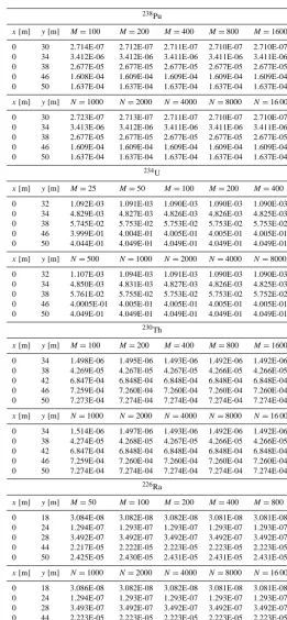
Table 3. Solution convergence of each species concentration at transect of inlet boundary (x=0) for four-species radionuclide trans-port problem considering simulated domain ofL=250 m,W=100 m, subject to Bateman-type sources located at 40 m≤y≤60 m for

t=1000 s year (M=number of terms summed for inverse generalized integral transform;N=number of terms summed for inverse fi-nite Fourier cosine transform). When we investigate the requiredM for inverse generalized integral transform,N=16 000 for the finite Fourier cosine transform inverse are used. When we investigate the requiredNfor inverse finite Fourier cosine transform,M=1600 for the generalized transform inverse are used.

238_Pu

x[m] y[m] M=100 M=200 M=400 M=800 M=1600

0 30 2.714E-07 2.712E-07 2.711E-07 2.710E-07 2.710E-07

0 34 3.412E-06 3.412E-06 3.411E-06 3.411E-06 3.411E-06

0 38 2.677E-05 2.677E-05 2.677E-05 2.677E-05 2.677E-05

0 46 1.608E-04 1.609E-04 1.609E-04 1.609E-04 1.609E-04

0 50 1.637E-04 1.637E-04 1.637E-04 1.637E-04 1.637E-04

x[m] y[m] N=1000 N=2000 N=4000 N=8000 N=16 000

0 30 2.723E-07 2.713E-07 2.711E-07 2.710E-07 2.710E-07

0 34 3.413E-06 3.412E-06 3.411E-06 3.411E-06 3.411E-06

0 38 2.677E-05 2.677E-05 2.677E-05 2.677E-05 2.677E-05

0 46 1.609E-04 1.609E-04 1.609E-04 1.609E-04 1.609E-04

0 50 1.637E-04 1.637E-04 1.637E-04 1.637E-04 1.637E-04

234_U

x[m] y[m] M=25 M=50 M=100 M=200 M=400

0 32 1.092E-03 1.091E-03 1.090E-03 1.090E-03 1.090E-03

0 34 4.829E-03 4.827E-03 4.826E-03 4.826E-03 4.825E-03

0 38 5.745E-02 5.753E-02 5.753E-02 5.753E-02 5.753E-02

0 46 3.999E-01 4.004E-01 4.005E-01 4.005E-01 4.005E-01

0 50 4.044E-01 4.049E-01 4.049E-01 4.049E-01 4.049E-01

x[m] y[m] N=500 N=1000 N=2000 N=4000 N=8000

0 32 1.107E-03 1.094E-03 1.091E-03 1.090E-03 1.090E-03

0 34 4.850E-03 4.831E-03 4.827E-03 4.826E-03 4.825E-03

0 38 5.761E-02 5.755E-02 5.753E-02 5.753E-02 5.752E-02

0 46 4.0005E-01 4.005E-01 4.005E-01 4.005E-01 4.005E-01

0 50 4.049E-01 4.049E-01 4.049E-01 4.049E-01 4.049E-01

230_Th

x[m] y[m] M=100 M=200 M=400 M=800 M=1600

0 34 1.498E-06 1.495E-06 1.493E-06 1.492E-06 1.492E-06

0 38 4.269E-05 4.267E-05 4.267E-05 4.266E-05 4.266E-05

0 42 6.847E-04 6.848E-04 6.848E-04 6.848E-04 6.848E-04

0 46 7.259E-04 7.260E-04 7.260E-04 7.260E-04 7.260E-04

0 50 7.273E-04 7.274E-04 7.274E-04 7.274E-04 7.274E-04

x[m] y[m] N=1000 N=2000 N=4000 N=8000 N=16 000

0 34 1.514E-06 1.497E-06 1.493E-06 1.492E-06 1.492E-06

0 38 4.274E-05 4.268E-05 4.267E-05 4.266E-05 4.266E-05

0 42 6.847E-04 6.848E-04 6.848E-04 6.848E-04 6.848E-04

0 46 7.259E-04 7.260E-04 7.260E-04 7.260E-04 7.260E-04

0 50 7.274E-04 7.274E-04 7.274E-04 7.274E-04 7.274E-04

226_Ra

x[m] y[m] M=50 M=100 M=200 M=400 M=800

0 18 3.084E-08 3.082E-08 3.082E-08 3.081E-08 3.081E-08

0 24 1.294E-07 1.293E-07 1.293E-07 1.293E-07 1.293E-07

0 28 3.492E-07 3.492E-07 3.492E-07 3.492E-07 3.492E-07

0 44 2.217E-05 2.222E-05 2.223E-05 2.223E-05 2.223E-05

0 50 2.425E-05 2.430E-05 2.431E-05 2.431E-05 2.431E-05

x[m] y[m] N=1000 N=2000 N=4000 N=8000 N=16 000

0 18 3.086E-08 3.082E-08 3.082E-08 3.081E-08 3.081E-08

0 24 1.294E-07 1.293E-07 1.293E-07 1.293E-07 1.293E-07

0 28 3.493E-07 3.492E-07 3.492E-07 3.492E-07 3.492E-07

0 44 2.223E-05 2.223E-05 2.223E-05 2.223E-05 2.223E-05

740 J.-S. Chen et al.: An analytical model for simulating two-dimensional multispecies plume migration

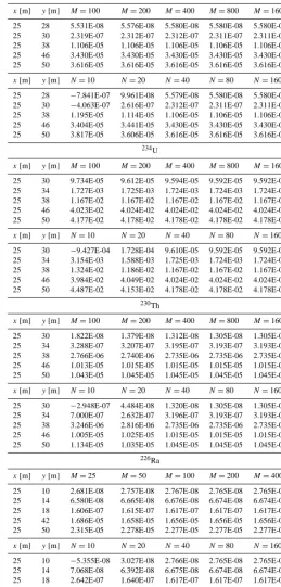
Table 4. Solution convergence of each species concentration at transect of x=25 m for four-species radionuclide transport problem considering simulated domain ofL=250 m,W=100 m, subject to Bateman-type sources located at 40 m≤y≤60 m fort=1000 year (M=number of terms summed for inverse generalized integral transform;N= number of terms summed for inverse finite Fourier cosine transform). When we investigate the requiredMfor inverse generalized integral transform,N=160 for the finite Fourier cosine transform inverse are used. When we investigate the requiredNfor inverse finite Fourier cosine transform,M=1600 for the generalized transform inverse are used.

238_Pu

x[m] y[m] M=100 M=200 M=400 M=800 M=1600

25 28 5.531E-08 5.576E-08 5.580E-08 5.580E-08 5.580E-08

25 30 2.319E-07 2.312E-07 2.312E-07 2.311E-07 2.311E-07

25 38 1.106E-05 1.106E-05 1.106E-05 1.106E-05 1.106E-05

25 46 3.430E-05 3.430E-05 3.430E-05 3.430E-05 3.430E-05

25 50 3.616E-05 3.616E-05 3.616E-05 3.616E-05 3.616E-05

x[m] y[m] N=10 N=20 N=40 N=80 N=160

25 28 −7.841E-07 9.961E-08 5.579E-08 5.580E-08 5.580E-08

25 30 −4.063E-07 2.616E-07 2.312E-07 2.311E-07 2.311E-07

25 38 1.195E-05 1.114E-05 1.106E-05 1.106E-05 1.106E-05

25 46 3.404E-05 3.441E-05 3.430E-05 3.430E-05 3.430E-05

25 50 3.817E-05 3.606E-05 3.616E-05 3.616E-05 3.616E-05

234_U

x[m] y[m] M=100 M=200 M=400 M=800 M=1600

25 30 9.734E-05 9.612E-05 9.594E-05 9.592E-05 9.592E-05

25 34 1.727E-03 1.725E-03 1.724E-03 1.724E-03 1.724E-03

25 38 1.167E-02 1.167E-02 1.167E-02 1.167E-02 1.167E-02

25 46 4.023E-02 4.024E-02 4.024E-02 4.024E-02 4.024E-02

25 50 4.177E-02 4.178E-02 4.178E-02 4.178E-02 4.178E-02

x[m] y[m] N=10 N=20 N=40 N=80 N=160

25 30 −9.427E-04 1.728E-04 9.610E-05 9.592E-05 9.592E-05

25 34 3.154E-03 1.588E-03 1.725E-03 1.724E-03 1.724E-03

25 38 1.324E-02 1.186E-02 1.167E-02 1.167E-02 1.167E-02

25 46 3.984E-02 4.049E-02 4.024E-02 4.024E-02 4.024E-02

25 50 4.487E-02 4.153E-02 4.178E-02 4.178E-02 4.178E-02

230_Th

x[m] y[m] M=100 M=200 M=400 M=800 M=1600

25 30 1.822E-08 1.379E-08 1.312E-08 1.305E-08 1.305E-08

25 34 3.288E-07 3.207E-07 3.195E-07 3.193E-07 3.193E-07

25 38 2.766E-06 2.740E-06 2.735E-06 2.735E-06 2.735E-06

25 46 1.013E-05 1.015E-05 1.015E-05 1.015E-05 1.015E-05

25 50 1.043E-05 1.045E-05 1.045E-05 1.045E-05 1.045E-05

x[m] y[m] N=10 N=20 N=40 N=80 N=160

25 30 −2.948E-07 4.484E-08 1.320E-08 1.305E-08 1.305E-08

25 34 7.000E-07 2.632E-07 3.196E-07 3.193E-07 3.193E-07

25 38 3.246E-06 2.816E-06 2.735E-06 2.735E-06 2.735E-06

25 46 1.005E-05 1.025E-05 1.015E-05 1.015E-05 1.015E-05

25 50 1.134E-05 1.035E-05 1.045E-05 1.045E-05 1.045E-05

226_Ra

x[m] y[m] M=25 M=50 M=100 M=200 M=400

25 10 2.681E-08 2.757E-08 2.767E-08 2.765E-08 2.765E-08

25 14 6.580E-08 6.665E-08 6.676E-08 6.674E-08 6.674E-08

25 18 1.606E-07 1.615E-07 1.617E-07 1.617E-07 1.617E-07

25 42 1.686E-05 1.658E-05 1.656E-05 1.656E-05 1.656E-05

25 50 2.315E-05 2.278E-05 2.277E-05 2.277E-05 2.277E-05

x[m] y[m] N=10 N=20 N=40 N=80 N=160

25 10 −5.355E-08 3.027E-08 2.766E-08 2.765E-08 2.765E-08

25 14 7.068E-08 6.392E-08 6.675E-08 6.674E-08 6.674E-08

25 18 2.642E-07 1.640E-07 1.617E-07 1.617E-07 1.617E-07

25 42 1.624E-05 1.655E-05 1.656E-05 1.656E-05 1.656E-05

J.-S. Chen et al.: An analytical model for simulating two-dimensional multispecies plume migration 741

10

0 20 40 60 80

x [m] 10-9

10-8 10-7 10-6 10-5 10-4 10-3 10-2 10-1 100 101

R

e

la

ti

v

e

c

o

n

c

e

n

tr

a

ti

o

n

10-9 10-8 10-7 10-6 10-5 10-4 10-3 10-2 10-1 100 101

0 20 40 60 80

Analytical solution Numerical solution

C1 C2 C3

C4 C5

0 20 40 60 80

x [m] 10-3

10-2 10-1 100 101

R

el

a

ti

v

e

co

n

ce

n

tr

a

ti

o

n

10-3 10-2 10-1 100 101

0 20 40 60 80

Analytical solution Numerical solution

C6 C7

C8 C9

C10

Fig. 8

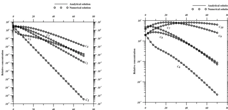
Figure 8. Comparison of spatial concentration profiles of ten-species alongx direction att=20 days obtained from derived analytical solutions and numerical solutions for the test example 3 of ten species decay chain used by Srinivasan and Clement (2008b).

terms for evaluating analytical solutions to the desired ac-curacies. Two-dimensional four-member radionuclide decay chain 238Pu→234U→230Th→226Ra is considered herein as convergence test example 1 to demonstrate the conver-gence behavior of the series expansions. This converconver-gence test example 1 is modified from a one-dimensional radionu-clide decay chain problem originated by Higashi and Pig-ford (1980) and later applied by van Genuchten (1985) to il-lustrate the applicability of their derived solution. The impor-tant model parameters related to this test example are listed in Tables 1 and 2. The inlet source is chosen to be symmet-rical with respect to thex-axis and conveniently arranged in the 40 m≤y≤60 m segment at the inlet boundary.

In order to determine the optimal term number of series expansions for the finite Fourier cosine transform inverse to achieve accurate numerical evaluation, we specify a suffi-ciently large number of series expansions for the generalized transform inverse so that the influence of the number of se-ries expansions for the generalized integral transform inverse on convergence of series expansion for finite Fourier cosine transform inverse can be excluded. A similar concept is used when investigating the required number of terms in the series expansions for the generalized integral transform inverse. An alternative approach is conducted by simultaneously varying the term numbers of series expansions for the generalized integral transform inverse and the finite Fourier cosine trans-form inverse.

Tables 3, 4 and 5 give results of the convergence tests up to 3 decimal digits of the solution computations along the three transects (inlet boundary atx=0 m,x=25 m, and exit boundary atx=250 m). In these tablesMandNare defined as the numbers of terms summed for the generalized integral transform inverse and finite Fourier cosine transform inverse, respectively. It is observed thatMandN are related closely to the true values of the solutions. For smaller true values, the

solutions must be computed with greaterMandN. However, convergences can be drastically speeded up if lower calcula-tion precision (e.g. 2 decimal digits accuracy) is acceptable. For example,(M, N )=(100 200)is sufficient for 2 decimal digits accuracy, while for 3 decimal digits accuracy we need (M, N )=(1600,8000). Two decimal digits accuracy is ac-ceptable for most practical problems. It is also found thatM increases andN decreases with increasingx.

To further examine the series convergence behavior, exam-ple 2 considers a transport system of large aspect ratio (_WL =

2500 m

100 m)and a narrower source segment, 45 m≤y≤55 m, on the inlet boundary. Tables 6 and 7 present results of the con-vergence tests of the solution computations along two tran-sects (inlet boundary and x=250 m). Tables 6 and 7 also show similar results for the dependences ofMandN onx. Note that largerM andN are required for each species in this test example, suggesting that the evaluation of the solu-tion for a large aspect ratio requires more series expansion terms to achieve the same accuracy as compared to example 1. Detailed results of the convergence test examples 1 and 2 are provided in the Supplement.

Using the required numbers determined from the conver-gence test, the computational time for evaluation of the so-lutions at 50 different observations only takes 3.782, 11.325, 23.95 and 67.23 s computer clock time on an Intel Core i7-2600 3.40 MHz PC for species 1, 2, 3, and 4 in the compari-son of example 1.

3 Results and discussion

3.1 Comparison of the analytical solutions with the numerical solutions

742 J.-S. Chen et al.: An analytical model for simulating two-dimensional multispecies plume migration

Figure 9. Effects of physical processes and chemical reactions on the concentration contours of four-species att=1000 years obtained from derived analytical solutions for four-member decay chain238Pu→234U→230Th→226Ra.

J.-S. Chen et al.: An analytical model for simulating two-dimensional multispecies plume migration 743

Table 5. Solution convergence of each species concentration at transect of exit boundary (x=250 m) for four-species radionuclide trans-port problem considering simulated domain of L=250 m, W=100 m subject to Bateman-type sources located at 40 m≤y≤60 m for

t=1000 years (M=number of terms summed for inverse generalized integral transform andN=number of terms summed for inverse finite Fourier cosine transform). When we investigate the requiredMfor inverse generalized integral transform,N=16 for the finite Fourier cosine transform inverse are used. When we investigate the requiredN for inverse finite Fourier cosine transform,M=6400 for the gener-alized transform inverse are used.

226_Ra

x[m] y[m] M=400 M=800 M=1600 M=3200 M=6400 250 2 2.289E-08 1.842E-08 1.814E-08 1.812E-08 1.812E-08 250 14 5.617E-08 5.060E-08 5.025E-08 5.022E-08 5.022E-08 250 26 1.528E-07 1.420E-07 1.413E-07 1.413E-07 1.413E-07 250 38 3.757E-07 2.743E-07 2.678E-07 2.674E-07 2.674E-07 250 50 1.645E-07 3.208E-07 3.306E-07 3.312E-07 3.312E-07

x[m] y[m] N=1 N=2 N=4 N=8 N=16 250 2 1.529E-07 −1.848E-09 1.892E-08 1.812E-08 1.812E-08 250 14 1.529E-07 5.348E-08 4.946E-08 5.022E-08 5.022E-08 250 26 1.529E-07 1.627E-07 1.414E-07 1.413E-07 1.413E-07 250 38 1.529E-07 2.666E-07 2.680E-07 2.674E-07 2.674E-07 250 50 1.529E-07 3.089E-07 3.303E-07 3.312E-07 3.312E-07

accuracy of the computer code. The first comparison exam-ple is the four-member radionuclide transport problem used in the convergence test example 1. The second comparison example considers the four-member radionuclide transport problem used in the convergence test example 2. The third comparison example is used to test the accuracy of the com-puter code for simulating the reactive contaminant transport of a long decay chain. The three comparison examples are ex-ecuted by comparing the simulated results of the derived ana-lytical solutions with the numerical solutions obtained using the Laplace transformed finite difference (LTFD) technique first developed by Moridis and Reddell (1991). A computer code for the LTFD solution is written in FORTTRAN lan-guage with double precision. The details of the FORTRAN computer code are described in Supplement.

Figures 2, 3 and 4 depicts the spatial concentration dis-tribution along one longitudinal direction (y=50 m) and two transverse directions (x=0 m and x=25 m) for con-vergence test example 1 att=1000 years obtained from an-alytical solutions and numerical solutions. Figures 5, 6 and 7 present the spatial concentration distribution along one lon-gitudinal direction (y=50 m) and two transverse directions (x=0 m andx=25 m) for the convergence test example 2 att=1000 years obtained from analytical solutions and nu-merical solutions. Excellent agreements between the two so-lutions for both examples are observed for a wide spectrum of concentration, thus warranting the accuracy and robust-ness of the developed analytical model.

The third example involves a 10 species decay chain previ-ously presented by Srinivasan and Clement (2008a) to eval-uate the performance of their one-dimensional analytical so-lutions. The relevant model parameters are summarized in

Tables 8 and 9. Our computer code is also compared against the LTFD solutions for this example. Figure 8 depicts the spatial concentration distribution att=20 days obtained an-alytically and numerically. Again there is excellent agree-ment between the analytical and numerical solutions, demon-strating the performance of our computer code for simulating transport problems with a long decay chain. The three com-parison results clearly establish the correctness of the analyt-ical model and the accuracy and capability of the computer code.

3.2 Assessing physical and chemical parameters on the radionuclide plume migration

Physical processes and chemical reactions affect the extent of contaminant plumes, as well as concentration levels. To illustrate how the physical processes and chemical reac-tions affect multispecies plume development, we consider the four-member radionuclide decay chain used in the pre-vious convergence test and solution verification. The model parameters are the same, except that the longitudinal (DL) and transverse (DT)dispersion coefficients are varied. Three sets of longitudinal and transverse dispersion coefficients DL=1000,DT=100;DL=1000,DT=200;DL=2000, DT=200 (all in m2year−1) are tested, all for a simulation time of 1000 years.

744 J.-S. Chen et al.: An analytical model for simulating two-dimensional multispecies plume migration

Table 6. Solution convergence of each species concentration at transect of inlet boundary (x=0 m) for four-species radionuclide trans-port problem considering simulated domain ofL=2500 m,W=100 m subject to Bateman-type sources located at 45 m≤y≤55 m for

t=1000 years (M= number of terms summed for inverse generalized integral transform;N= number of terms summed for inverse fi-nite Fourier cosine transform). When we investigate the requiredM for inverse generalized integral transform,N=12 800 for the finite Fourier cosine transform inverse are used. When we investigate the requiredNfor inverse finite Fourier cosine transform,M=6400 for the generalized transform inverse are used.

238_Pu

x[m] y[m] M=400 M=800 M=1600 M=3200 M=6400

0 36 5.395E-07 5.391E-07 5.389E-07 5.387E-07 5.387E-07

0 38 1.908E-06 1.908E-06 1.908E-06 1.907E-06 1.907E-06

0 42 1.640E-05 1.642E-05 1.642E-05 1.642E-05 1.642E-05

0 46 1.203E-04 1.199E-04 1.198E-04 1.198E-04 1.198E-04

0 50 1.522E-04 1.524E-04 1.525E-04 1.525E-04 1.525E-04

x[m] y[m] N=2000 N=4000 N=8000 N=16 000 N=32 000

0 36 5.392E-07 5.389E-07 5.388E-07 5.387E-07 5.387E-07

0 38 1.908E-06 1.908E-06 1.907E-06 1.907E-06 1.907E-06

0 42 1.642E-05 1.642E-05 1.642E-05 1.642E-05 1.642E-05

0 46 1.198E-04 1.198E-04 1.198E-04 1.198E-04 1.199E-04

0 50 1.525E-04 1.525E-04 1.525E-04 1.525E-04 1.525E-04

234_U

x[m] y[m] M=800 M=1600 M=3200 M=6400 M=12 800

0 36 4.817E-04 4.815E-04 4.815E-04 4.814E-04 4.814E-04

0 38 2.348E-03 2.348E-03 2.348E-03 2.348E-03 2.348E-03

0 44 1.011E-01 1.012E-01 1.012E-01 1.012E-01 1.012E-01

0 48 3.704E-01 3.705E-01 3.705E-01 3.705E-01 3.705E-01

0 50 3.862E-01 3.864E-01 3.864E-01 3.864E-01 3.864E-01

x[m] y[m] N=4000 N=8000 N=16 000 N=32 000 N=64 000

0 36 4.818E-04 4.816E-04 4.815E-04 4.814E-04 4.814E-04

0 38 2.348E-03 2.348E-03 2.348E-03 2.348E-03 2.348E-03

0 44 1.013E-01 1.013E-01 1.012E-01 1.012E-01 1.012E-01

0 48 3.705E-01 3.705E-01 3.705E-01 3.705E-01 3.705E-01

0 50 3.864E-01 3.864E-01 3.864E-01 3.864E-01 3.864E-01

230_Th

x[m] y[m] M=400 M=800 M=1600 M=3200 M=6400

0 40 3.429E-06 3.427E-06 3.424E-06 3.423E-06 3.423E-06

0 42 1.773E-05 1.783E-05 1.782E-05 1.782E-05 1.782E-05

0 44 1.028E-04 1.089E-04 1.093E-04 1.093E-04 1.093E-04

0 48 7.095E-04 7.089E-04 7.090E-04 7.090E-04 7.090E-04

0 50 7.210E-04 7.205E-04 7.206E-04 7.206E-04 7.206E-04

x[m] y[m] N=2000 N=4000 N=8000 N=16 000 N=32 000

0 40 3.430E-06 3.425E-06 3.424E-06 3.423E-06 3.423E-06

0 42 1.783E-05 1.782E-05 1.782E-05 1.782E-05 1.782E-05

0 44 1.093E-04 1.093E-04 1.093E-04 1.093E-04 1.093E-04

0 48 7.090E-04 7.090E-04 7.090E-04 7.090E-04 7.090E-04

0 50 7.206E-04 7.206E-04 7.206E-04 7.206E-04 7.206E-04

226_Ra

x[m] y[m] M=400 M=800 M=1600 M=3200 M=6400

0 24 3.557E-08 3.556E-08 3.556E-08 3.555E-08 3.555E-08

0 28 9.276E-08 9.274E-08 9.273E-08 9.273E-08 9.273E-08

0 40 2.159E-06 2.159E-06 2.159E-06 2.159E-06 2.159E-06

0 44 7.739E-06 7.809E-06 7.813E-06 7.813E-06 7.813E-06

0 50 2.072E-05 2.082E-05 2.083E-05 2.084E-05 2.084E-05

x[m] y[m] N=1000 N=2000 N=4000 N=8000 N=16 000

0 24 3.559E-08 3.557E-08 3.556E-08 3.555E-08 3.555E-08

0 28 9.278E-08 9.275E-08 9.274E-08 9.273E-08 9.273E-08

0 40 2.159E-06 2.159E-06 2.159E-06 2.159E-06 2.159E-06

0 44 7.815E-06 7.814E-06 7.813E-06 7.813E-06 7.813E-06

J.-S. Chen et al.: An analytical model for simulating two-dimensional multispecies plume migration 745

Table 7. Solution convergence of each species concentration at transect ofx=250 m for four-species radionuclide transport problem con-sidering simulated domain of L=2500 m,W=100 m subject to Bateman-type sources located at 45 m≤y≤55 m fort=1000 years (M=number of terms summed for inverse generalized integral transform;N=number of terms summed for inverse finite Fourier cosine transform). When we investigate the requiredMfor inverse generalized integral transform,N=160 for the finite Fourier cosine transform inverse are used. When we investigate the requiredNfor inverse finite Fourier cosine transform,M=12 800 for the generalized transform inverse are used.

238_Pu

x[m] y[m] M=200 M=400 M=800 M=1600 M=3200

25 32 2.578E-08 2.569E-08 2.564E-08 2.563E-08 2.563E-08

25 34 1.153E-07 1.162E-07 1.161E-07 1.161E-07 1.161E-07

25 40 3.485E-06 3.661E-06 3.661E-06 3.661E-06 3.661E-06

25 46 2.262E-05 2.176E-05 2.163E-05 2.163E-05 2.163E-05

25 50 2.752E-05 2.920E-05 2.929E-05 2.929E-05 2.929E-05

x[m] y[m] N=10 N=20 N=40 N=80 N=160

25 32 −7.217E-07 4.318E-08 2.558E-08 2.563E-08 2.563E-08

25 34 −1.422E-06 1.470E-07 1.162E-07 1.161E-07 1.161E-07

25 40 4.741E-06 3.665E-06 3.661E-06 3.661E-06 3.661E-06

25 46 2.175E-05 2.155E-05 2.163E-05 2.163E-05 2.163E-05

25 50 2.713E-05 2.938E-05 2.929E-05 2.929E-05 2.929E-05

234_U

x[m] y[m] M=200 M=400 M=800 M=1600 M=3200

25 34 3.937E-05 4.038E-05 4.022E-05 4.019E-05 4.019E-05

25 36 2.029E-04 2.162E-04 2.160E-04 2.159E-04 2.159E-04

25 42 5.649E-03 7.897E-03 7.936E-03 7.936E-03 7.936E-03

25 46 2.695E-02 2.593E-02 2.565E-02 2.564E-02 2.564E-02

25 50 2.913E-02 3.552E-02 3.585E-02 3.586E-02 3.586E-02

x[m] y[m] N=10 N=20 N=40 N=80 N=160

25 34 −2.184E-03 1.134E-04 4.038E-05 4.019E-05 4.019E-05

25 36 −2.113E-03 1.975E-04 2.158E-04 2.159E-04 2.159E-04

25 42 1.118E-02 8.092E-03 7.936E-03 7.936E-03 7.936E-03

25 46 2.580E-02 2.544E-02 2.564E-02 2.564E-02 2.564E-02

25 50 3.262E-02 3.608E-02 3.586E-02 3.586E-02 3.586E-02

230_Th

x[m] y[m] M=800 M=1600 M=3200 M=6400 M=12 800

25 36 3.192E-08 3.181E-08 3.180E-08 3.179E-08 3.179E-08

25 38 1.578E-07 1.576E-07 1.576E-07 1.576E-07 1.576E-07

25 44 3.838E-06 3.914E-06 3.914E-06 3.914E-06 3.914E-06

25 48 8.531E-06 8.539E-06 8.539E-06 8.539E-06 8.539E-06

25 50 9.253E-06 9.261E-06 9.261E-06 9.262E-06 9.262E-06

x[m] y[m] N=10 N=20 N=40 N=80 N=160

25 36 −6.448E-07 2.862E-08 3.167E-08 3.179E-08 3.179E-08

25 38 −1.271E-07 1.141E-07 1.577E-07 1.576E-07 1.576E-07

25 44 4.705E-06 3.925E-06 3.914E-06 3.914E-06 3.914E-06

25 48 7.869E-06 8.534E-06 8.540E-06 8.539E-06 8.539E-06

25 50 8.345E-06 9.353E-06 9.261E-06 9.262E-06 9.262E-06

226_Ra

x[m] y[m] M=100 M=200 M=400 M=800 M=1600

25 12 1.268E-08 1.273E-08 1.272E-08 1.272E-08 1.272E-08

25 18 4.817E-08 4.822E-08 4.821E-08 4.821E-08 4.821E-08

25 26 2.830E-07 2.824E-07 2.824E-07 2.824E-07 2.824E-07

25 42 8.794E-06 7.484E-06 7.578E-06 7.579E-06 7.579E-06

25 50 1.761E-05 1.449E-05 1.494E-05 1.497E-05 1.497E-05

x[m] y[m] N=10 N=20 N=40 N=80 N=160

25 12 8.791E-08 1.264E-08 1.272E-08 1.272E-08 1.272E-08

25 18 −1.512E-07 4.713E-08 4.821E-08 4.821E-08 4.821E-08

25 26 5.221E-07 2.830E-07 2.824E-07 2.824E-07 2.824E-07

25 42 7.960E-06 7.587E-06 7.578E-06 7.579E-06 7.579E-06

746 J.-S. Chen et al.: An analytical model for simulating two-dimensional multispecies plume migration

Table 8. Transport parameters used for verification example 2 involving the ten-species transport problem used by Srinivasan and

Clement (2008b).

Parameter Value

Domain length,L[m] 250

Domain width,W[m] 100

Seepage velocity,v[m year−1] 5

Longitudinal Dispersion coefficient,DL[m2year−1] 50 Transverse Dispersion coefficient,DT[m2year−1] 50

Retardation coefficient,Rii=1, 2,. . . ,10 1.9, 1, 1.4, 1, 5, 8, 1.4, 3.1, 1, 1

Decay constant,ki[year−1]i=1, 2, . . . , 10 3, 2, 1.5, 1.25, 2.75, 1, 0.75, 0.5, 0.25, 0.1 Source decay constant,λm[year−1]m=1, 2,. . . ,10 0.1, 0.75, 0.5, 0.25, 0, 0, 0.3, 1, 0, 0.65

Table 9. Coefficients of Bateman-type boundary source for ten-species transport problem used by Srinivasan and Clement (2008b).

Species,i bim

m=1 m=2 m=3 m=4 m=5 m=6 m=7 m=8 m=9 m=10 Species 1 10

Species 2 0 5

Species 3 0 0 2.5

Species 4 0 0 0 0

Species 5 0 0 0 0 10

Species 6 0 0 0 0 0 5

Species 7 0 0 0 0 0 0 2.5

Species 8 0 0 0 0 0 0 0 0

Species 9 0 0 0 0 0 0 0 0 0

Species 10 0 0 0 0 0 0 0 0 0 0

plumes are confined within 60 m×50 m area in the simula-tion domain. The moderate mobility of238Pu reflects the fact that it is a medial sorbed member of this radionuclide de-cay chain. The high concentration level of234U accounts for the high first-order decay rate constant of its parent species 238_{Pu and its own low first-order decay rate constant. The} plume extents and concentration levels may be sensitive to longitudinal and transverse dispersion. Increase of the lon-gitudinal and/or transverse dispersion coefficients enhances the spreading of the plume extensively along the longitudinal and/or transverse directions, thereby lowering the plume con-centration level. Because the concon-centration levels of the four radionuclides are influenced by both source release rates and decay chain reactions, 230Th has the least extended plume area, while 226Ra has the greatest plume area for all three sets of dispersion coefficients. These dispersion coefficients only affect the size of plumes of the four radionuclide, but the order of their relative plume size remains the same (i.e. 226_{Ra >}238_{Pu >}234_{U >}230_{Th for the simulated condition).} Indeed, in the reactive contaminant transport, the chemical parameters of sorption and decay rate are more important than the physical parameters of dispersion coefficients that govern the order of the plume extents and the concentration levels.

3.3 Simulating the natural attenuation of chlorinated solvent plume migration

Natural attenuation is the reduction in concentration and mass of the contaminant due to naturally occurring processes in the subsurface environment. The process is monitored for regulatory purposes to demonstrate continuing attenuation of the contaminant reaching the site-specific regulatory goals within reasonable time, hence, the use of the term moni-tored natural attenuation (MNA). MNA has been widely ac-cepted as a suitable management option for chlorinated sol-vent contaminated groundwater. Mathematical models are widely used to evaluate the natural attenuation of plumes at chlorinated solvent sites. The multispecies transport analyti-cal model developed in this study provides an effective tool for evaluating performance of the monitoring natural attenua-tion of plumes at a chlorinated solvent site because a series of daughter products produced during biodegradation of chlori-nated solvent such as PCE→TCE→DCE→VC→ETH. Thus simulation of the natural attenuation of plumes a chlo-rinated solvent constitutes an attractive field application ex-ample of our multispecies transport model.

J.-S. Chen et al.: An analytical model for simulating two-dimensional multispecies plume migration 747

Table 10. Transport parameters used for example application

in-volving the five-species dissolved chlorinated solvent problem used by BIOCHLOR.

Parameter Value

Domain length,L[m] 330.7

Domain width,W[m] 213.4

Seepage velocity,v[m year−1] 34.0

Longitudinal dispersion coefficient,DL[m2year−1] 449 Transverse dispersion coefficient,DT[m2year−1] 44.9 Retardation coefficient,Ri[−]

PCE 7.13

TCE 2.87

DCE 2.8

VC 1.43

ETH 5.35

Decay constant,ki[year−1] PCE

TCE 1

DCE 0.7

VC 0.4

ETH 0

Source decay rate constant,λm[year−1]

PCE 0

TCE 0

DCE 0

VC 0

ETH 0

(Aziz et al., 2000) provided by the Center for Subsurface Modeling Support (CSMoS) of USEPA was the most com-monly used model. An illustrated example from BIOCHLOR manual (Aziz et al., 2000) is considered to demonstrate the application of the developed analytical model. This example application demonstrated that BIOCHLOR can reproduce plume movement from 1965 to 1998 at the contaminated site of Cape Canaveral Air Station, Florida. The simulation conditions and transport parameters for this example appli-cation are summarized in Table 10. Constant source centrations rather than exponentially declining source con-centration of five-species chlorinated solvents are specified in the 90.7 m≤y≤122.7 m segment at the inlet boundary (x=0). This means that the exponents (λim)of

Bateman-type sources in Eqs. (16a) or (16b) need to be set to zero for the constant source concentrations and source intensity con-stants (bim)are set to zero when subscriptidoes not equal to

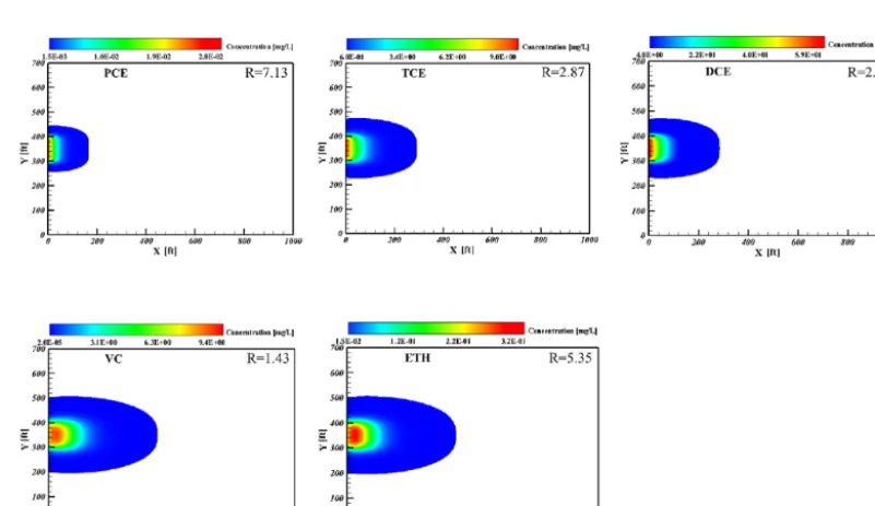
subscriptm. Table 11 lists the coefficients of Bateman-type boundary source used for this example application involving the five-species dissolved chlorinated solvent problem. Spa-tial concentration contours of five-species at t=1 year ob-tained from the derived analytical solutions for natural atten-uation of chlorinated solvent plumes are depicted in Fig. 10.

Table 11. Coefficients of Bateman-type boundary source used for

example application involving the five-species dissolved chlori-nated solvent problem used by BIOCHLOR.

Species,i bim

m=1 m=2 m=3 m=4 m=5 PCE,i=1 0.056

TCE,i=2 15.8

DCE,i=3 98.5

VC,i=4 3.08

ETH,i=5 0.03

It is observed that the mobility of plumes is quite sensitive to the species retardation factors, whereas the decay rate con-stants determine the plume concentration level. The plumes can migrate over a larger region for species having a low re-tardation factor such as VC. The low decay rate constants such as ETH have higher concentration distribution than the VC. It should be noted that a larger extent of plume observed for ETH in Fig. 10 is mainly attributed to the plume mass accumulation from the predecessor species VC that have a larger plume extent. The effect of high retardation of the ETH is hindered by the mass accumulation of the predeces-sor species VC.

4 Conclusions

prede-748 J.-S. Chen et al.: An analytical model for simulating two-dimensional multispecies plume migration

J.-S. Chen et al.: An analytical model for simulating two-dimensional multispecies plume migration 749

Appendix A: Derivation of analytical solutions

In this appendix, we elaborate on the mathematical proce-dures for deriving the analytical solutions.

The Laplace transforms of Eqs. (7a), (7b), (9)–(12) yield 1

P eL

∂2G1(X, Y, s)

∂X2

−∂G1(X, Y, s)

∂X + ρ2 P eT

∂2G1(X, Y, s)

∂Y2

−(R1s+κ1) G1(X, Y, s)=0 (A1a) 1

P eL

∂2_G

i(X, Y, s)

∂X2 −

∂Gi(X, Y, s)

∂X +

ρ2

P eT

∂2_G

i(X, Y, s)

∂Y2

−κiGi(X, Y, s)+κi−1Gi−1(X, Y, s)=RisGi

(X, Y, s) i=2,3, . . .N (A1b)

− 1

P eL

∂Gi(X=0, Y, s)

∂X +Gi(X=0, Y, s)

=Fi(s)[H (Y−Y1)−H (Y−Y2)] 0≤Y ≤1i=1. . .N. (A2) ∂Gi(X=1, Y, s)

∂X =0 0≤Y≤1 i=1. . .N. (A3)

∂Gi(X, Y=0, s)

∂Y =0 0≤X≤1 i=1. . .N. (A4)

∂Gi(X, Y=1, s)

∂Y =0 0≤X≤1 i=1. . .N. (A5)

wheresis the Laplace transform parameter, andGi(X, Y, s)

andFi(s)are defined by the Laplace transformation relations

as

Gi(X, Y, s)=

∞

Z

0

e−sTCi(X, Y, T )dT (A6)

Fi(s)=

∞

Z

0

e−sTfi(T )dT . (A7)

The finite Fourier cosine transform is used here because it satisfies the transformed governing equations in Eqs. (A1a) and (A2b) and their corresponding boundary conditions in Eqs. (A4) and (A5). Application of the finite Fourier cosine transform on Eqs. (A1)–(A3) leads to

1 P eL

d2H1(X, n, s)

∂X2 −

dH1(X, n, s) dX −

R1s+κ1+

ρ2n2π2 P eT

H1(X, n, s)=0 (A8a) 1

P eL

d2Hi(X, n, s)

dX2 −

dHi(X, n, s)

dX −

Ris+κi+ ρ2n2π2

P eT

Hi(X, n, s)+κi−1Hi−1(X, n, s)=0 (A8b)

− 1

P eL

dHi(X=0, n, s)

dX +Hi(X=0, n, s)=Fi(s)8(n) (A9)

dHi(X=1, n, s)

dX =0 (A10)

where8(n)=

_Y

2−Y1n=0 sin(nπ Y2)−sin(nπ Y1)

nπ n=1,2,3. . .

,nis the fi-nite Fourier cosine transform parameter, Hi(X, n, s) is

de-fined by the following conjugate equations (Sneddon, 1972)

Hi(X, n, s)=

1

Z

0

Gi(X, Y, s)cos(nπ Y )dY (A11)

Gi(X, Y, s)=Hi(X, n=0, s) +2

n=∞

X

n=1

Hi(X, n, s)cos(nπ Y ) . (A12)

Using changes-of-variables, similar to those applied by Chen and Liu (2011), the advective terms in Eqs. (A8a) and (A8b) as well as nonhomogeneous terms in Eq. (A9) can be easily removed. Thus, substitutions of the change-of-variable into Eqs. (A8a), (A8b), (A9) and (A10) result in diffusive-type equations associated with homogeneous boundary con-ditions

1 P eL

d2U1(X, n, s)

dX2 −

R1s+κ1+ ρ2n2π2

P eT

+P eL

4

U1(X, n, s)

=e− P e_L

2 X

R1s+κ1+

ρ2n2π2 P eT

F1(s)8(n) (A13a) 1

P eL

d2Ui(X, n, s)

dX2 −

_{P e}

L

4 +Ris+κ1+ ρ2n2π2

P eT

Ui(X, n, s)

=e−P e2LX

Ris+κi+

ρ2n2π2 P eT

Fi(s)8(n)

−e−P e2LX_{κi−1Fi−1(s)8(n)}−κi−1Ui−1(X, n, s) (A13b)

−dUi(X=0, n, s)

dX +

P e

2 Ui(X=0, n, s)=0 (A14) dUi(X=1, n, s)

dX +

P eL

2 Ui(X=1, n, s)=0 (A15) where Ui(X, n, s) is defined as the following

change-of-variable relation

Hi(X, n, s)=Fi(s)8(n)+e P e_L

2 X_{Ui(X, n, s). (A16)}

As detailed in Ozisik (1989), the generalized integral transform pairs for Eqs. (A13a) and (A13b) and its associ-ated boundary conditions Eqs. (A14) and (A15) are defined as

Zi(ξl, n, s)=

1

Z

0

750 J.-S. Chen et al.: An analytical model for simulating two-dimensional multispecies plume migration

Ui(X, n, s)=

∞

X

l=1

K(ξl, X) N (ξl)

Zi(ξl, n, s) (A18)

where K(ξl, X)=P e₂Lsin(ξlX)+ξlcos(ξlX) is the kernel

function, N (ξl)= _{P e}2 2 L

4 +P eL+ξl2

,ξl is the eigenvalue,

deter-mined from the equation

ξlcotξl− ξ_l2 P eL

+P eL

4 =0. (A19)

The generalized integral transforms of Eqs. (13a) and (13b) give

− R1s+κ1+ ρ2n2π2

P eT

+P eL

4 +

ξ_l2 P eL

!

Zi(ξl, n, s)

=

R1s+κ1+

ρ2n2π2 P eT

F1(s)8(n)2 (ξl) (A20)

− Ris+κi+ ρ2n2π2

P eT

+P eL

4 +

ξ_l2 P eL

!

Zi(ξl, n, s)

=

Ris+κi+

ρ2n2π2 P eT

Fi(s)8(n)2 (ξl)−κi−1

Fi−1(s)8(n)2 (ξl)−κi−1Zi−1(ξl, n, s), (A21)

where2 (ξl)= _{P e}P e2Lξl L

4 +ξl2

.

Solving for Eqs. (A20) and (A21) algebraically for each species,Zi(ξl, n, s), in sequence, leads to

Z1(ξl, n, s)= −

s+α1−β1 s+α1

F1(s)8(n)2 (ξl) (A22) Z2(ξl, n, s)=

−s+α2−β2 s+α2

F2(s)

+ σ2β1

(s+α2) (s+α1) F1(s)

8(n)2 (ξl) (A23)

Z3(ξl, n, s)=

−s+α3−β3 s+α3

F3(s)+

σ3β2 (s+α3) (s+α2)

F2(s) σ3σ2β1

(s+α3) (s+α2) (s+α1) F1

8(n)2 (ξl) (A24)

Z4(ξl, n, s)=

−s+α4−β4 s+α4

F4(s)+

σ4β3 (s+α4) (s+α3)

F3(s)

+ σ4σ3β2

(s+α4) (s+α3) (s+α2) F2(s)

+ σ4σ3σ2β1

(s+α4) (s+α3) (s+α2) (s+α1)

F1(s)

8(n)2 (ξl) ,

(A25) whereαi(ξl)=_Riκi +ρ

2_n2_π2

P eTRi +

P eL

4Ri + ξ_l2

P eLRi,βi(ξl)=

P eL

4Ri + ξ_l2

P eLRi, σi=

κi−1

Ri . Upon inspection of Eqs. (A22)–(A25),

compact expressions valid for all species can be generalized as

Zi(ξl, n, s)=[Pi(ξl, n, s)

+Qi(ξl, n, s)]8(n)2 (ξl) i=1,2. . .N, (A26)

where Pi(ξl, n, s)= −s+_sαi+−αiβiFi(s) and Qi(ξl, n, s)= k=i−2

P

k=0

βi−k−1

j₁=k 5 j₁=0

σi−j1

j₂=k+1

5 j₂=0

s+αi−j₂

Fi−k−1(s).

The solutions in the original domain are obtained by a series of integral transform inversions in combination with changes-of-variables.

The inverse generalized integral transform of Eq. (A26) gives

Wi(X, n, s)=

∞

X

m=1

K(ξl, X) N (ξl)

[Pi(ξl, n, s)

+Qi(ξl, n, s)]8(n)2 (ξl) . (A27)

Using change-of-variable relation of Eq. (A16), one obtains

Hi(ξl, n, s)=Fi(s)8(n)+e P e_L

2 xD

∞

X

m=1

K(ξl, xD) N (ξl)

[Pi(ξl, n, s)+Qi(ξl, n, s)]8(n)2 (ξl) . (A28)

The finite Fourier cosine inverse transform of Eq. (A28) results in

Gi(X, Y, s)

=Fi(s)8(n=0)+e P eL

2 X·

∞

X

l=1

K(ξl, X) N (ξl)

[Pi(ξl, n, s)+Qi(ξl, n, s)]8(n=0)2 (ξl) +2

n=∞

X

n=1

(

Fi(s)8(n)+e P eL

2 X

∞

X

l=1

K(ξl, X) N (ξl)

[Pi(ξl, n, s)+Qi(ξl, n, s)]8(n)2 (ξl)}cos(nπ Y ) .

(A29) The analytical solutions in the original domain will be completed by taking the Laplace inverse transform of Eq. (A29).Pi(ξl, n, s)in Eq. (29) is in the form of the

prod-uct of two functions. The Laplace transform of s+_sαi_+αi−βi can be easily obtained as

L−1

_s+α i−βi s+αi

=δ(T )−βie−αiT (A30)

Thus, the Laplace inverse ofPi(ξl, n, s)can be achieved

using the convolution theorem as

pi(ξl, n, T )=L−1[Pi(ξl, n, s)]=L−1

−s+αi−βi

s+αi

Fi(s)

J.-S. Chen et al.: An analytical model for simulating two-dimensional multispecies plume migration 751

= −fi(T )+βie−αiT T Z

0

fi(τ )eαiτdτ. (A31)

The Laplace inverse ofQi(ξl, n, s)can be also approached

using the similar method. By taking Laplace inverse trans-form onQi(ξl, n, s), we have

qi(ξl, n, T )=L−1[Qi(ξl, n, s)]

=L−1



   

k=i−2

X

k=0

βi−k−1

j1=k

5 j1=0

σi−j1

j2=k+1

5 j2=0

s+αi−j2

Fi−k−1(s)

     = k=i−2

X

k=0 βi−k−1

j1=k

5 j1=0

σi−j1L

−1      1

j2=k+1

5 j2=0

s+αi−j2

Fi−k−1(s)

     (A32)

Expressing _j 1

2=k+1

5 j2=0

s+αi−j2

as the summation of partial frac-tions and applying the inverse Laplace transform formula, one gets L−1      1

j2=k+1

5 j2=0

s+αi−j2

    

=L−1



   

j2=k+1

6 j2=0

1

j3=i

5 j3=i−k−1,j36=i−j2

(αj3−αi−j2) s+αi−j2

    

=j2

=k+1 6 j2=0

e−αi−j₁T j3=i

5 j3=i−k−1,j36=i−j1

(αj3−αi−j1)

(A33)

Recall that the inverse Laplace transform of Fi−k−1(s) is fi−k−1(T ). Thus, the Laplace inverse transform of

1

j₂=k+1

5 j₂=0

s+αi−j2

Fi−k−1(s)in Eq. (1) can be achieved using the convolution integral equation as

L−1      1

j2=k+1

5 j2=0

s+αi−j2

Fi−k−1(s)

     = j2=k+1

X

j2=0

e−αi−j1T

T R

0

eαi−j1τ_{fi−k−1(τ )dτ}

j3=i

5 j3=i−k−1,j36=i−j2

αj3−αi−j2

(A34)

Putting Eq. (A34) into Eq. (A2) we can obtain the follow-ing form:

qi(ξl, n, T )= k=i−2

X

k=0 βi−k−1

j1=k

5 j1=0

σi−j1

j2=k+1

X

j2=0

e−αi−j₁T T R

0

eαi−j₁τ_f

i−k−1(τ )dτ

j3=i

5 j3=i−k−1,j36=i−j2

αj3−αi−j2

. (A35)

Thus, the final solution can be expressed as Eq. (13) with the corresponding functions defined in Eqs. (14) and (15).

Note that Eq. (A33) is invalid for some of αi−j2

be-ing identical. For such conditions, we can still reduce 1

j₂=k+1

5 j₂=0 s

+αi−j₂

to a sum of partial fraction expansion. How-ever, it will lead to different Laplace inverse formulae. For example, the following formulae is used for allαi−j2 being

identical L−1      1

j2=k+1

5 j2=0

s+αi−j      =T

k_e−αi−j₂T

k! . (A36)

The generalized formulae for the cases with some ofαi−j2

being identical will not be provided herein because there are a large number of combinations ofαi−j2. We suggest that