GlobWat – a global water balance model to assess water use in irrigated agriculture

www.hydrol-earth-syst-sci.net/19/3829/2015/ doi:10.5194/hess-19-3829-2015

© Author(s) 2015. CC Attribution 3.0 License.

GlobWat – a global water balance model to assess

water use in irrigated agriculture

J. Hoogeveen1,3, J.-M. Faurès1, L. Peiser1, J. Burke2, and N. van de Giesen3 1_{Food and Agriculture Organization of the United Nations, Rome, Italy}

2_{World Bank, Washington, D.C., USA}

3_{Delft University of Technology, Delft, the Netherlands}

Correspondence to: J. Hoogeveen (jippe.hoogeveen@fao.org)

Received: 1 December 2014 – Published in Hydrol. Earth Syst. Sci. Discuss.: 20 January 2015 Accepted: 9 August 2015 – Published: 10 September 2015

Abstract. GlobWat is a freely distributed, global soil water balance model that is used by the Food and Agriculture Or-ganization (FAO) to assess water use in irrigated agriculture, the main factor behind scarcity of freshwater in an increas-ing number of regions. The model is based on spatially dis-tributed high-resolution data sets that are consistent at global level and calibrated against values for internal renewable wa-ter resources, as published in AQUASTAT, the FAO’s global information system on water and agriculture. Validation of the model is done against mean annual river basin outflows.

The water balance is calculated in two steps: first a “ver-tical” water balance is calculated that includes evaporation from in situ rainfall (“green” water) and incremental evap-oration from irrigated crops. In a second stage, a “horizon-tal” water balance is calculated to determine discharges from river (sub-)basins, taking into account incremental evapora-tion from irrigaevapora-tion, open water and wetlands (“blue” water). The paper describes the methodology, input and output data, calibration and validation of the model. The model results are finally compared with other global water balance models to assess levels of accuracy and validity.

1 Introduction

Modelling of the world’s hydrological cycle is important to assess, among others, water resources availability and the sustainability of their use, the impact of climate change, and the influence on global food production (Wood et al., 2011). With regard to global food production, one of the major ques-tions on the future of irrigated agriculture is whether there will be sufficient freshwater to satisfy the growing needs of agricultural and non-agricultural users. Agriculture accounts for about 70 % of the freshwater withdrawals in the world (FAO, 2013), while consumptive use of water in agricul-ture (water that is evaporated on irrigated fields) accounts for about 90 % of all of the water that is evaporated as a result of human intervention. Irrigated agriculture is therefore the main component of water demand and a driver of scarcity of freshwater in an increasing number of regions.

in irrigation. The Global Map of Irrigation Areas provides information about the distribution of land under irrigation, but data collection through AQUASTAT country surveys has shown that country statistics for agricultural water with-drawals are not always available, and when they exist, they are often unreliable. In most cases they are rough estimates based on water use per unit area of land equipped for irriga-tion.

Actual water use in annual water balances is changing over time as cropping patterns and cropping intensities shift and change, sometimes in response to available water resources. Therefore a consistent global picture of water withdrawals and consumptive use in irrigated agriculture cannot be ob-tained without some reference to modelled estimates. Sim-ulation of water use in irrigated agriculture at global scale at the highest available resolution would therefore address a gap in hydrological understanding under contemporary land and water use patterns.

A number of global models exist that simulate water use in agriculture. WaterGAP (Döll and Fiedler, 2008; Hunger and Döll, 2008; Alcamo et al., 2007), WBMplus (Wisser et al., 2010), GEPIC (Liu, 2009; Liu and Yang, 2010), LPJmL (Bie-mans, 2012; Rost et al., 2008) and PCR-GLOBWB (Wada et al., 2014) are all global hydrological models that have been used to calculate water use by irrigated agriculture. Most of these models are sophisticated hydrological models that are used for detailed water balance analyses in which consump-tive water use in agriculture is only one of the components of the water balance rather than the main focus of analysis. Almost all of them are developed at a spatial disaggregation (30 arcmin or coarser) which is not directly comparable with the heterogeneity and spatial variability of irrigation as cap-tured in the FAO’s high-resolution (5 arcmin) Global Map of Irrigation Areas or in other global agriculture land use data such as that available through FAO and IIASA’s Global Agro-Ecological Zones portal (FAO/IIASA, 2012).

To overcome this incompatibility between global hydro-logical models and the Global Map of Irrigation Areas, Siebert and Döll (2008, 2010) developed the Global Crop Water Model (GCWM) to calculate irrigated crop water re-quirements on a grid resolution of 5 arcmin by using the MIRCA2000 data set (Portmann et al., 2008). However, con-trary to the earlier mentioned models, the GCWM does not simulate the influence of incremental crop evapotranspiration on the hydrological cycle to the extent that model results can be calibrated or validated on river discharges.

Therefore, in order to be able to estimate current and fu-ture water use in agriculfu-ture objectively and the consequent impact on river basin mean annual flow, a global water bal-ance model, GlobWat, was developed. The defining feature of the model is that it is based on a set of spatially differ-entiated data sets at 5 arcmin resolution that are consistent at global level, and that model outputs are validated against actual basin outflows.

The model is designed to complement other FAO data sets and models as used for AQUASTAT (FAO, 2013), Global Agro-Ecological Zones (FAO/IIASA, 2012) and Global Per-spective Studies (FAO, 2006, 2011a).

2 Methodology

Precipitation provides part of the water crops’ need to satisfy their transpiration requirements. The soil stores part of the precipitation water, which is later evaporated or transpired by plants. In humid climates, the water stored by the soil is sufficient to ensure satisfactory growth in rainfed agriculture. Instead, in climates with extended dry periods, irrigation is necessary to compensate for the evaporation deficit due to insufficient precipitation. The purpose of the modelling ex-ercise is to estimate net irrigation water requirements on ir-rigated land. In terms of a hydrological balance, this is in-cremental evaporation due to the import of water onto land. Net irrigation water requirements in irrigation are calculated as the volume of water needed to compensate for the deficit between potential crop evaporation and effective precipita-tion over the growing period of the crop. This requirement varies considerably with climatic conditions, seasons, crops and soil types. Following Savenije (2004), the model descrip-tion uses the term evaporadescrip-tion (E) to describe evaporative processes originating from soil evaporation, transpiration and interception. In agro-hydrology these processes are often re-ferred to as evapotranspiration (ET).

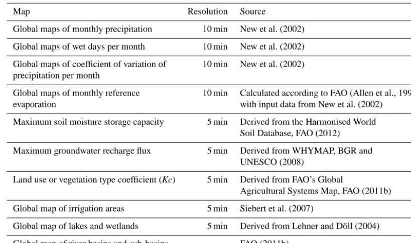
GlobWat has spatially distributed input and output layers consisting of monthly precipitation, number of wet days per month, coefficient of variation of precipitation, monthly ref-erence evaporation, maximum soil moisture storage capacity, maximum groundwater recharge flux, irrigated areas, land use, and areas of open water and wetlands. All these input layers are based on freely available spatial data sets with a resolution of 10 arcmin for the climate data sets and 5 arcmin for all the terrain and land data sets (details and references of the data sets are given in Table 3).

horizon-tal water balances helps to clarify discussions on “green” and “blue” water (Falkenmark and Rockström, 2004), as well as on water footprints (Hoekstra and Chapagain, 2007), since it can distinguish between evaporation attributable to land management (evaporation from in situ rainfall) and evapora-tion attributable to water management (evaporaevapora-tion resulting from the lateral import of water). The significance of open water and wetlands as evaporative “sinks” is also made ex-plicit. A schematic representation of these two calculation steps is given in Fig. 1.

Under long-term, stationary conditions (therefore ignoring changes in hydrological storage), the model is based on two simple equations. For the vertical water balance,

P +Eincr-irr=Erain+Eincr-irr+RO+R, (1) and for the horizontal (surface) water balance,

Qout=Qin+RO+R−Eincr-irr−Eincr-OW−Eincr-wetl, (2) whereP is precipitation (L3T−1),Erainis rainfed evapora-tion (L3T−1), Qin is inflow (L3T−1), RO is (sub-)surface runoff (L3T−1),Ris groundwater recharge (in step 1)/base-flow (in step 2) (L3T−1),Eincr-irris incremental evaporation from irrigation (L3T−1),Eincr-OWis incremental evaporation over open water (L3T−1),Eincr-wetl is incremental evapora-tion over wetlands (L3T−1) andQoutis outflow (L3T−12), whereLis length andT is time.

The detailed calculations procedure for the respective model components is explained below.

3 Soil water balance

The soil water balance model is similar to the Thornwaite and Mather procedure (Steenhuis and Van der Moolen, 1986) adapted for daily time steps. The basic soil water balance equation for this model is as follows:

P =Erain+R+RO+1S/1t, (3)

with P =precipitation (mm day−1), Erain= rainfall-dependent evaporation (mm day−1), R=groundwater recharge (mm day−1), RO=(sub-)surface runoff (mm day−1), 1S=changes in soil moisture storage (mm) and1t=time step (day).

The computation of water balance is carried out on a spa-tial resolution of 5 arcmin grid cells and in daily time steps taking account of spatial variations in rainfall, evaporative power of the atmosphere and soil properties.

4 Precipitation

Daily precipitation is generated from monthly figures by us-ing a mixed Bernoulli gamma distribution function (Wilks and Wilby, 1999). First the number of wet days is randomly

distributed over the month by using a Bernoulli distribution, and then the amount of monthly precipitation is randomly distributed over the wet days by using a gamma distribution with parameters derived from the data set with coefficients of variation of precipitation.

Usually, precipitation generators use Markov chains to generate precipitation events (Schoof and Pryor, 2008). How-ever, the data sets used do not include information to param-eterise these Markov chains. To take into consideration that the chance of rainfall after a wet day is higher than the chance of rainfall after a dry day, the following simple adjustment was made:

Pwet wet=(1+corr)×Pwet mean (4)

and

Pwet dry=Pwet mean×(1−Pwet wet) / (1−Pwet mean) , (5) withPwet wetis the probability of a wet day after a wet day, Pwet dry is the probability of a wet day after a dry day, and Pwet mean is the average probability of a wet day calculated as

Pwet mean=wet days/days of the month. (6) corr=correction coefficient is calculated as

corr=0.5×(days of the month−wet days)/days of the month. (7) Applying this adjustment, the chance of a wet day after a wet day is almost 1.5 times as high when the number of wet days approaches 0, while the chance of a wet day after a wet day approaches the average chance of a wet day if the number of wet days is high.

The spatial distribution of all climate data is determined by the CRU CL 2.0 data set (New et al., 2002). This data set has been chosen to obtain maximum consistency between precipitation and reference evaporation, and because it de-scribes average climatic conditions, which are comparable to the data available in AQUASTAT.

5 Rainfall-dependent evaporation

Δ

S

P

E

R

R

R

Q

E

E

E

P = Precipitation

ΔS = Changes in storage

Erain = Rainfed evaporation RO = (Sub-)surface runoff

R = Groundwater recharge (in Step 1) / Baseflow (in Step 2)

Qin = Inflow

Eincr-irr = Incremental Evaporation from irrigation Eincr-OW = Incremental Evaporation over open water Eincr-wetl = Incremental Evaporation over wetlands

Qout = Outflow

Step 1:

‘Vertical’ water balance

Step 2:

‘Horizontal’ water balance

E

Q

R

Figure 1. Schematic representation of modelling steps.

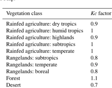
Table 1. Vegetation types derived from FAO’s Global Agricultural

Systems Map.

Vegetation class Kc factor

Rainfed agriculture: dry tropics 0.9 Rainfed agriculture: humid tropics 1 Rainfed agriculture: highlands 0.9 Rainfed agriculture: subtropics 1 Rainfed agriculture: temperate 1 Rangelands: subtropics 0.8 Rangelands: temperate 0.9 Rangelands: boreal 0.8

Forest 1.1

Desert 0.7

Other 1

In equations:

Erain(t )=Kc×Eo(t )forSmax≥S(t−1)≥Seav (8) Erain(t )=Kc×Eo(t )×S(t−1)/ (Seav)forS(t−1) < Seav (9)

Seav=0.5×Smax (10)

Smax=Rtd×SCmax (11)

witht the time step indicator,Erain(t )the rainfed evapora-tion ont (mm day−1),Eo(t )the reference evaporation ont (mm day−1),Kcthe crop or land use factor (–),S(t−1) the

available soil moisture on t−1 (mm), Smax the maximum soil moisture storage (mm), Seav the easily available soil moisture (mm), Rtdthe effective root depth (m), and SCmax the maximum soil moisture storage capacity (mm m−1_).

The crop or land use factorKcis not constant over the year. It varies during the growing season, depending on the grow-ing stage. However, for rainfed conditions, differentiatedKc factors were not applied, since no distinction was made be-tween the different crops and their cropping calendars. The Kc factors used were attributed to the Global Agricultural Systems Map (FAO, 2011b) according to Table 1.

As can be seen from the equations above, the easily avail-able soil moisture (Seav) is defined as half the maximum soil moisture storage (Smax). In reality, easily available moisture depends on the type of plant, its growing stage and its soil type, and it varies from about 40 to 60 % of the maximum soil moisture storage capacity (SCmax) (Raes et al., 2012). For a global model, 50 % can be considered a reasonable ap-proximation.

The spatial distribution of the maximum soil moisture storage capacity (SCmax) was derived from the Harmonised World Soil Database (FAO, 2012).

are different ways to estimate the effective root depth, i.e. half the maximum root depth (Evans et al., 1996) or the soil depth in which 90 % of the weight of the roots is found (Allen et al., 1998; FAO, 1978). However, for a global model, such information is not available and therefore an initial effective rooting depth of 60 cm is assumed. Since the results of model computation are very sensitive to effective rooting depth and to soil moisture storage capacity (SCmax), both parameters were used to calibrate the model.

6 Groundwater recharge, actual available soil moisture and (sub-)surface runoff

Groundwater recharge is assumed to occur only above a threshold level when there is enough water available in the soil to percolate downward in the model. The recharge rate depends on a maximum possible groundwater recharge flux, which is derived from the Groundwater Resources of the World Map provided by the World-wide Hydrogeological Mapping and Assessment Programme (WHYMAP) (BGR and UNESCO, 2008), and is assumed to be proportional to the available soil moisture. The recharge component is as-sumed to contribute to the shallow groundwater circulation that appears as effluent seepage in the annually renewable water resource account of the respective basins. Given that all groundwater heads are generated by tectonic uplift and fluvial erosion, all groundwater flows in the model are as-sumed to enter the annual river basin balance and not enter permanent groundwater storage.

In equations:

R(t )=Rmax×(S(t−1)−Seav) / (Smax−Seav)

forSmax≥S(t−1)≥Seav, (12)

R(t )=0 forS(t−1) < Seav, (13) withR(t )the recharge flux ont (mm day−1_{) andR}

max the maximum groundwater recharge flux (mm day−1_).

The available soil moisture is calculated per day by adding ingoing and outgoing fluxes to the available soil moisture of the day before. Runoff occurs when the balance of the ingo-ing and outgoingo-ing fluxes exceeds the maximum soil moisture storage capacity.

In equations:

B(t )=S(t−1)+(P (t )−Erain(t )−RO(t ))·1t (14) IfB(t ) < Smax, then

S(t )=B(t ), (15)

RO(t )=0. (16)

IfB(t )≥Smax, then

S(t )=Smax, (17)

RO(t )=(B(t )−Smax) /1t, (18)

withB(t ) the balance on t (mm), RO(t )the (sub-)surface runoff ont (mm day−1) andS(t )the available soil moisture ont (mm).

7 Evaporation for crops under irrigation

Evaporation for crops under irrigation is calculated by mul-tiplying reference evaporation by a crop and growing stage specific factor according to the FAO Penman–Monteith method (Allen et al., 1998). It is assumed that there is always enough water available to ensure that crops under irrigation never suffer water stress.

The evaporation of a crop under irrigation (Ec) is calcu-lated as follows:

Ec(t )=Kc×Eo(t ), (19)

with Ec(t ) crop evaporation under irrigation on t (mm day−1),Eo(t )reference evaporation on t (mm day−1) andKcthe rop or land use factor (–).

Crop coefficients (Kc) have been derived for four differ-ent growing stages: the initial phase (just after sowing), the development phase, the mid-phase and the late phase (when the crop is ripening to be harvested). In general, these co-efficients are low during the initial phase, after which they increase during the development phase to high values in the mid-phase, and again decrease in the late phase. It is assumed that the initial phase, the development phase and the late phase each take 1 month for each crop, while the duration of the mid-phase varies according to the type of crop. For example, the growing season for wheat in Morocco starts in October and ends in April, as follows: initial phase: October (Kc=0.4); development phase: November (Kc=0.8); mid-phase: December–March (Kc=1.15); and late phase: April (Kc=0.3).

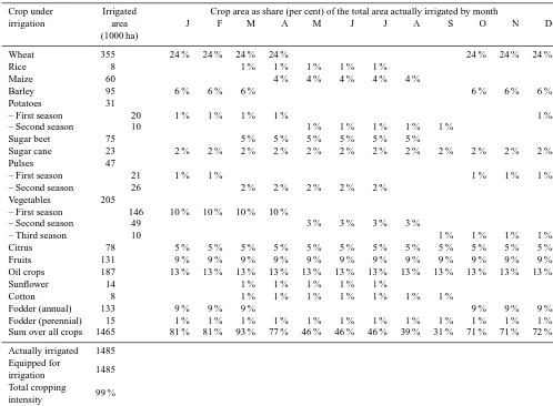
Evaporation requirements of crops in irrigated agriculture are calculated by converting data of irrigated area by crop (at the national level) into a cropping calendar with monthly oc-cupation rates of the land equipped for irrigation. Cropping calendars have been developed by AQUASTAT (http://www. fao.org/nr/water/aquastat/water_useagr/index2.stm) for each of the countries or country groups of the study (except for China, India and the United States, which were divided into several zones of homogenous cropping patterns). Table 2 presents the irrigation cropping calendar for Morocco, de-rived from AQUASTAT data for the year 2004.

Ec-total(t )=IA×6c(CIc×Ec(t )) , (20) with Ec-total(t ) total evaporation for all crops under irriga-tion ontin mm day−1,IAthe area equipped for irrigation as percentage of cell area for the given grid cell,ccrop under irrigation,6cthe sum over the different crops,CIcthe crop-ping intensity for cropcandEc(t )the crop evaporation ont in mm day−1_{, varying for each crop and each growth stage.}

The difference between the calculated evaporation of the irrigated area,Ec, and the evaporation provided by rainfall, Erain, is equal to the incremental evaporation due to irriga-tion, which equals the net irrigation water requirement: Eincr-irr(t )=Ec-total(t )−Erain(t ), (21) withEincr-irr(t )the incremental evaporation due to irrigation ont(mm day−1).

8 Evaporation from open water and swamps

A special correction is applied for grid cells existing of open water or swamps. In these areas, the actual evaporation de-pends on heat storage in lakes and reservoirs, which is related to the depth of the water bodies, and, in the case of swamps and wetlands, the vegetation. In the model, evaporation from open water is computed in a simplified manner as follows:

Eow(t )=Kow×Eo(t ) (22)

and

B(t )=(P (t )−Eow(t ))·1t, (23) with Eow(t ) actual evaporation over open water on t (mm day−1),Kowthe open water coefficient (–) andB(t )the open water balance ont(mm).

IfB(t ) <0, then

RO(t )=0, (24)

Erain(t )=P (t ), (25)

Eincr-ow(t )=(−1×B(t ))/1t. (26)

IfB(t )≥0, then

RO(t )=B(t )/1t, (27)

Erain(t )=Eow(t )/1t, (28)

Eincr-ow(t )=0, (29)

withEincr-ow(t )the incremental evaporation over open water ont(mm day−1).

Evaporation over swamps and wetlands is calculated sep-arately, but in the same way as evaporation over open water. For this study, open water evaporation and evaporation over swamps and wetlands is assumed to be 10 % higher than ref-erence evaporation (Kow=1.1).

The spatial distribution of open water and wetlands was derived from the global map of lakes and wetlands (Lehner and Döll, 2004).

It was decided to make a distinction between the rainfall-dependent evaporation over open water and incremental evaporation over open water, to make it possible to distin-guish between evaporation of water that is available from the “vertical” water balance (the rainfall minus evaporation) and the water that has to come from outside the spatial domain of calculation (the incremental evaporation).

9 River basin discharges

To calculate discharges from river basins and sub-basins, a global map of river basins was used which was developed in the framework of the FAO’s study “The state of the world’s land and water resources for food and agriculture – manag-ing systems at risk” (FAO, 2011b). For this study, major river basins and their sub-basins were delineated from the Hy-droSHEDS database. Sub-basins were named and assigned a flow direction, indicating the sub-basin directly downstream of each sub-basin. Aggregated water balances were calcu-lated on a monthly time step by subtracting all evaporation occurring over the sub-basin from the sum of the total pre-cipitation over the sub-basin and the inflow from upstream basins (Eq. 30).

Bsb(t )=Qin(t )+ X

P (t )−XE(t ) (30)

withBsbthe water balance of aggregated grid cells in a sub-basin (m3month−1), t the time step indicator, Qin the in-coming flow in the sub-basin calculated as the sum of the outflow from all upstream sub-basins (m3month−1), P

P the precipitation summed over all grid cells in the sub-basin (m3month−1) andP

Ethe total evaporation summed over all grid cells in the sub-basin (m3month−1).

There is a lag between the time water enters a sub-basin and the time it gets out, and some of the inflow is trapped in storage in the sub-basin. To take the time lag and storage ef-fect into account, a simple linear reservoir model (De Zeeuw, 1973) is used to calculate monthly values for river discharges and the amount of water stored per sub-basin:

Ssb(t )=Ssb(t−1)+(Bsb(t )−Qout(t−1))·1t (31) and

Qout(t )=Ssb(t )×F (32)

withSsb the river sub-basin storage (m3),1t the time step (month),Qoutthe outflow from the sub-basin (m3month−1) andF the response factor (1/month).

Table 2. Cropping calendar in irrigation for Morocco for the year 2004.

Crop under Irrigated Crop area as share (per cent) of the total area actually irrigated by month

irrigation area J F M A M J J A S O N D

(1000 ha)

Wheat 355 24 % 24 % 24 % 24 % 24 % 24 % 24 %

Rice 8 1 % 1 % 1 % 1 % 1 %

Maize 60 4 % 4 % 4 % 4 % 4 %

Barley 95 6 % 6 % 6 % 6 % 6 % 6 %

Potatoes 31

– First season 20 1 % 1 % 1 % 1 % 1 %

– Second season 10 1 % 1 % 1 % 1 % 1 %

Sugar beet 75 5 % 5 % 5 % 5 % 5 % 5 %

Sugar cane 23 2 % 2 % 2 % 2 % 2 % 2 % 2 % 2 % 2 % 2 % 2 % 2 %

Pulses 47

– First season 21 1 % 1 % 1 % 1 % 1 %

– Second season 26 2 % 2 % 2 % 2 % 2 %

Vegetables 205

– First season 146 10 % 10 % 10 % 10 %

– Second season 49 3 % 3 % 3 % 3 %

– Third season 10 1 % 1 % 1 % 1 %

Citrus 78 5 % 5 % 5 % 5 % 5 % 5 % 5 % 5 % 5 % 5 % 5 % 5 %

Fruits 131 9 % 9 % 9 % 9 % 9 % 9 % 9 % 9 % 9 % 9 % 9 % 9 %

Oil crops 187 13 % 13 % 13 % 13 % 13 % 13 % 13 % 13 % 13 % 13 % 13 % 13 %

Sunflower 14 1 % 1 % 1 % 1 % 1 %

Cotton 8 1 % 1 % 1 % 1 % 1 % 1 % 1 %

Fodder (annual) 133 9 % 9 % 9 % 9 % 9 % 9 %

Fodder (perennial) 15 1 % 1 % 1 % 1 % 1 % 1 % 1 % 1 % 1 % 1 % 1 % 1 % Sum over all crops 1465 81 % 81 % 93 % 77 % 46 % 46 % 46 % 39 % 31 % 71 % 71 % 72 %

Actually irrigated 1485 Equipped for

1485 irrigation

Total cropping

99 % intensity

outflow can be equal to the monthly inflow andF will be 1. Large sub-basins or sub-basins with high storage capacity have high retention times and therefore low values for the response factorF. For all sub-basins in this study a response factorF of 0.3 was assumed. No differentiation was made between different carry-over factors since analysing monthly differences in stream flow was beyond the scope of the study.

10 Irrigation efficiencies

GlobWat calculates the incremental evaporation over areas under irrigation. In the case of paddy rice, an additional ume of water is used for flooding to control weeds. This vol-ume of water can be calculated by multiplying the area under irrigated paddy rice by a water layer of 20 cm. The total irri-gation requirements can then be calculated as follows: Irrreq= Eincr-irr(yr)×Acell+0.2×Apaddy(yr)×10, (33) with Irrreq the total irrigation requirements per year (m3), Eincr-irr(yr) the incremental evaporation due to irrigation per

year (mm),Acellthe area of the grid cell (ha) andApaddy(yr) the harvested area under paddy irrigation per year (ha).

Table 3. Input data sets.

Map Resolution Source

Global maps of monthly precipitation 10 min New et al. (2002)

Global maps of wet days per month 10 min New et al. (2002)

Global maps of coefficient of variation of 10 min New et al. (2002) precipitation per month

Global maps of monthly reference 10 min Calculated according to FAO (Allen et al., 1998)

evaporation with input data from New et al. (2002)

Maximum soil moisture storage capacity 5 min Derived from the Harmonised World Soil Database, FAO (2012)

Maximum groundwater recharge flux 5 min Derived from WHYMAP, BGR and UNESCO (2008)

Land use or vegetation type coefficient (Kc) 5 min Derived from FAO’s Global

Agricultural Systems Map, FAO (2011b)

Global map of irrigation areas 5 min Siebert et al. (2007)

Global map of lakes and wetlands 5 min Derived from Lehner and Döll (2004)

Global map of river basins and sub-basins FAO (2011b)

The average of the years for which cropping calendar data are available is 2004, and consequently the calculated out-puts of GlobWat as presented here are on average valid for that year. Water withdrawal data in AQUASTAT that were estimated on the basis of earlier model calculations were ex-cluded from the exercise.

Irrigation efficiencies can be calculated by applying Eq. (35) per country for those countries for which coun-try data on agricultural water withdrawals are available. For those countries for which no water withdrawal data are avail-able, irrigation efficiencies have been estimated based on countries nearby with similar conditions with regard to cli-mate and economic development:

Irreff=Irrreq/Qaww, (35)

with Irreffthe irrigation efficiency (–), Irrreqthe total irriga-tion requirements (m3yr−1) andQawwthe agricultural water withdrawal (m3yr−1).

11 Input and output data sets

The input data sets used are derived from public domain data sets and are found in Table 3.

The results of the water balance calculations consist of monthly values by grid cell for generated precipitation, actual evaporation, incremental evaporation due to irrigated agricul-ture, surface runoff, groundwater recharge and water stored as soil moisture. Aggregated annual water balances can be calculated for any desired spatial domain (e.g. countries or river basins) and include, apart from the above-mentioned

variables, incremental evaporation over open water and in-cremental evaporation over wetlands.

12 Model results, calibration and validation

Water balances have been generated by the model and aggre-gated for each country to compare them with AQUASTAT data on Internal Renewable Water Resources (IRWR) and “Internally produced groundwater”. The internal renewable water resources of a country are defined as “Long-term aver-age annual flow of rivers and recharge of aquifers generated from endogenous precipitation”. It corresponds to the sum of surface runoff and groundwater recharge as calculated by the model. Internally produced groundwater is defined as “Long-term annual average groundwater recharge, generated from precipitation within the boundaries of the country”, which was compared to the model-generated groundwater recharge (AQUASTAT datadase; FAO, 2013).

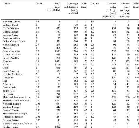
Table 4. Calibration factors per hydrological region.

Region Cal-sw IRWR Recharge Diff. Cal-gw Ground Ground Diff.

(mm) and drainage (mm) water water (mm)

AQUASTAT (mm), recharge recharge

modelled (mm) (mm),

AQUASTAT modelled

Northern Africa 1.5 9 8 0 1.5 3 2 0

Sudano–Sahel 2 19 38 20 1 7 6 −1

Gulf of Guinea 1.7 455 475 20 1.5 134 146 11

Central Africa 1.9 353 409 56 1.2 156 185 29

Eastern Africa 2 96 138 41 1.2 33 34 1

Southern Africa 2 57 101 44 1 17 24 7

Indian Ocean islands 1 571 590 20 1 94 109 15

North America 0.7 299 268 −31 2.5 92 84 −9

Mexico 1 210 206 −4 2.5 71 66 −5

Central America 0.7 1335 1306 −29 2.5 397 263 −134

Greater Antilles 0.9 440 389 −51 2.2 126 110 −15

Lesser Antilles 0.9 218 386 168 2.2 141 108 −33

Guyanas 0.9 1051 1109 58 2.5 512 333 −179

Andes 0.7 1106 1041 −64 2.5 278 194 −84

Brazil 1 638 761 123 2 221 311 91

South America 0.7 322 347 25 2.5 81 54 −27

Arabian Peninsula 2 2 7 4 2.5 2 0 −2

Caucasus 0.6 393 359 −34 2.5 151 72 −79

Iran 0.6 79 102 22 2.5 30 11 −20

Near East 0.7 181 163 −18 2.5 54 47 −7

Central Asia 0.7 57 73 16 2.5 9 22 13

South Asia 0.9 465 537 72 2.5 130 81 −49

East Asia 0.7 296 227 −69 2.5 77 57 −20

Mainland Southeast Asia 0.8 993 987 −5 2.5 326 200 −126

Maritime Southeast Asia 0.9 1323 1436 113 1 282 276 −6

Northern Europe 0.55 687 555 -133 2 120 112 −8

Western Europe 0.7 444 469 25 1 143 130 −13

Central Europe 0.75 228 223 −5 1 64 75 11

Mediterranean Europe 0.7 391 367 −24 2.4 89 97 9

Russian Federation 0.55 257 264 7 1.2 47 51 4

Eastern Europe 0.75 135 154 18 1 45 59 14

Australia and New Zealand 1 103 102 −1 1 9 11 1

Pacific Islands 0.7 1802 1779 −23 2 – – –

Calsw varies from 0.55 to 2 and Calgw from 1 to 2.5. The results of the calibration are presented in Table 4.

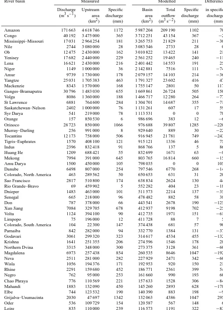
Validation of the model output was accomplished by com-paring average river discharges of the Global River Dis-charge Database (Center for Sustainability and the Global Environment, 2014). The stations with discharge data in the Global River Discharge Database are not always located at the mouth of the river basin. Therefore the specific discharge, defined as the total annual discharge divided by the area over which the discharge is generated, was calculated for the stations situated as close as possible to the mouth of the river. The specific discharges per station were then compared with the specific discharge per river basin as derived from the modelled data. Table 5 shows the result of this

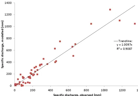
valida-tion exercise for 51 river basins with an area greater than 100 000 km2. Figure 2 shows the same results in a graph.

The total area weighted average specific discharge as mea-sured over the above-listed river basins is 332 mm per year. The area weighted average difference (observed minus simu-lated) in specific discharges is 2 mm, which indicates that the model underestimates the total discharge over all river basins by 0.7 %.

Table 5. Validation results per river basin.

River basin Measured Modelled Difference

Discharge Upstream Specific Basin Total Specific in specific (m3s−1) area discharge area outflow discharge discharge (km2) (mm) (km2) (m3s−2) (mm) (mm)

Amazon 171 663 4 618 746 1172 5 987 204 209 190 1102 70

Congo 40 192 3 475 000 365 3 712 251 43 154 367 −2

Mississippi–Missouri 17 031 2 964 254 181 3 265 753 21 829 211 −30

Nile 2744 3 080 000 28 3 083 546 2733 28 0

Ob 12 475 2 430 000 162 3 010 822 13 422 141 21

Yenisey 17 682 2 440 000 229 2 561 252 19 465 240 −11

Lena 16 621 2 430 000 216 2 401 442 14 553 191 25

Niger 1149 1 000 000 36 2 142 881 7516 111 −74

Amur 9739 1 730 000 178 2 079 157 14 103 214 −36

Yangtze 25 031 1 705 383 463 1 791 327 23 602 416 47

Mackenzie 8343 1 570 000 168 1 755 147 2801 50 117

Ganges–Bramaputra 30 796 1 483 030 655 1 669 861 26 724 505 150

Volga 8086 1 360 000 188 1 466 717 12 280 264 −77

St Lawrence 6881 764 600 284 1 304 701 14 687 355 −71

Saskatchewan–Nelson 2402 1 000 000 76 1 131 261 607 17 59

Syr Darya 541 219 000 78 1 113 531 0 0 78

Orange 157 850 530 6 986 696 383 12 −6

Orinoco 28 723 850 000 1066 976 688 39 807 1285 −220

Murray–Darling 256 991 000 8 929 640 889 30 −22

Tocantins 12 173 758 000 506 916 945 21 781 749 −243

Tigris–Euphrates 1570 408 100 121 915 121 1336 46 75

Indus 2396 832 418 91 868 766 137 5 86

Huang He 1209 688 421 55 832 699 1671 63 −8

Mekong 7994 391 000 645 803 765 16 814 660 −15

Amu Darya 1500 450 000 105 798 035 0 0 105

Danube 6498 807 000 254 797 546 6770 268 −14

Colorado, North America 463 289 562 50 650 653 631 31 20

Sao Francisco 2817 510 800 174 638 834 2624 130 44

Rio Grande–Bravo 69 459 902 5 552 282 404 23 −18

Dnieper 1483 463 000 101 511 573 2214 137 −35

Senegal 665 218 000 96 478 482 882 58 38

Don 787 378 000 66 443 541 2678 190 −125

Xun Jiang 7084 329 705 678 412 937 9198 702 −25

Volta 1124 394 100 90 412 735 1971 151 −61

Limpopo 75 196 000 12 411 728 88 7 5

Colorado, South America 104 22 300 147 374 438 681 57 90

Parnaiba 842 282 000 94 332 770 1384 131 −37

Godavari 3061 299 320 323 314 617 4534 455 −132

Krishna 1641 251 355 206 274 596 1546 178 28

Northern Dvina 3315 348 000 300 273 375 3128 361 −60

Magdalena 6973 257 438 854 260 535 8646 1047 −192

Neva 2511 281 000 282 227 929 2471 342 −60

Wisla 1056 194 376 171 192 953 920 150 21

Rhine 2291 159 680 452 186 771 2361 399 54

Negro 762 95 000 253 161 660 990 193 60

Chao Phraya 776 110 569 221 157 633 1528 306 −84

Mahandi 1883 132 090 450 145 260 2893 628 −178

Elbe 744 123 532 190 140 390 883 198 −9

Grijalva–Usumacinta 2030 47 697 1342 132 063 4386 1047 295

Oder 536 109 729 154 120 587 567 148 6

y = 1.0097x R² = 0.9087

0 200 400 600 800 1000 1200 1400

0 200 400 600 800 1000 1200 1400

Speci

fic

d

isc

h

ar

ge,

modell

ed

(mm)

Specific discharge, observed (mm)

Trendline:

Figure 2. Graphic representation of validation results in which

modelled specific river discharges are compared to observed spe-cific river discharges.

mean square error–standard deviation ratio (RSR) of 0.31 (the RSR can vary from the optimal value of 0 – no residual variation, so perfect simulation – to a large positive value). According to Moriasi et al. (2007), model simulation can be judged as satisfactory if NSE>0.50, PBIAS<±25 %, and RSR<0.70.

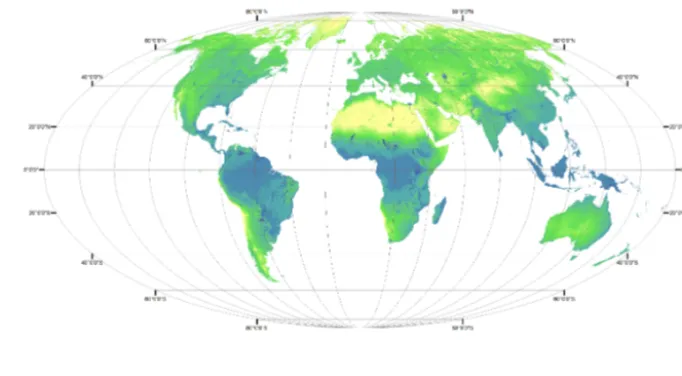
The outputs of the model are global raster maps with a res-olution of 5 arcmin containing monthly information on gen-erated precipitation, total actual evaporation from the soil water balance component, incremental evaporation from ir-rigation, incremental evaporation from lakes and wetlands, (sub-)surface runoff and groundwater recharge. The output maps are available on FAO’s AQUAMAPS website: http: //www.fao.org/nr/water/aquamaps/.

As an example, Fig. 3 shows total yearly actual evapora-tion (the sum of actual evaporaevapora-tion from the soil water bal-ances and incremental evaporation from irrigated areas, lakes and wetlands).

Figure 4 shows the calculated accumulated outflow per sub-basin. Since the HydroSHEDS database does not pro-vide data above 60◦ northern latitude, and due to the fact that in these areas population densities are generally low, the mapped sub-basins are of a lower spatial resolution, which can be seen in Greenland and the northern-flowing river basins in Siberia (e.g. Ob, Lena, Yenissey).

Apart from maps, the model also calculates aggregated results per country, per major basin and per sub-basin. As an example, the total global water balance as calculated by GlobWat is presented in Table 6.

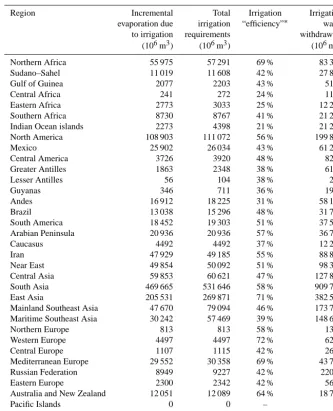
In Table 7, incremental evaporation due to irrigation as calculated by GlobWat; total irrigation water require-ments; amounts of water withdrawn for irrigation as avail-able in AQUASTAT (http://www.fao.org/nr/water/aquastat/ data/query/index.html); and irrigation efficiencies, are pre-sented for the hydrological regions. Since more or less reli-able water withdrawal data per country are availreli-able for less

Table 6. Global terrestrial water balance.

109m3 (mm)

Precipitation 105 316 (805)

Rainfed evaporation 61 106 (467) Renewable water resources 44 211 (338) Incremental evaporation over open water 1184 (9) Incremental evaporation over wetlands 2899 (22) Incremental evaporation from irrigation 1268 (10)

Outflow to sea 38 859 (297)

than 50 % of the countries included in this analysis, it was de-cided to present water use efficiency values for hydrological regions only rather than for individual countries.

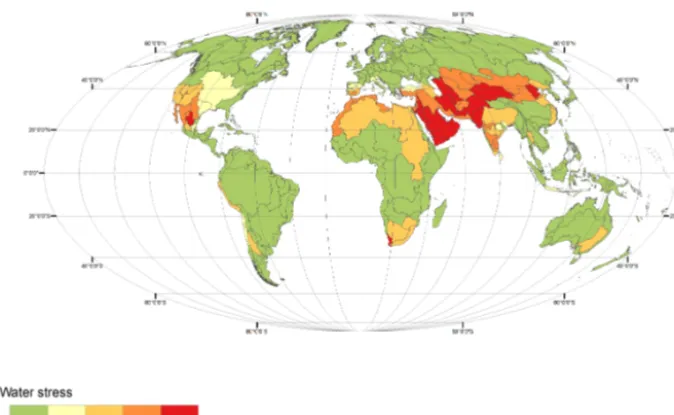
Figure 5 shows the distribution of global water stress by major river basin based on incremental evaporation caused by irrigation as a percentage of total generated groundwater and surface water resources. Levels of water stress are of-ten classified by using the Millennium Development Goals – Water Indicator. The MDG Water Indicator measures water stress per country on the ratio between total water withdrawn and total renewable water resources (UN, 2008; FAO, 2013). Using this indicator, it is estimated that a withdrawal rate above 20 % of renewable water resources represents “sub-stantial” pressure on water resources, while more than 40 % is considered “critical” (FAO 2011b). Other classifications use thresholds of 0–10 % no stress, 10–20 %, low stress, 20– 40 % moderate stress, and more than 40 % severe stress (UN, 1997). The mentioned stress classifications include all water withdrawals. Taking into account that agriculture accounts for more than 90 % of the consumptive use of global wa-ter withdrawals (FAO, 2012), and that on average incremen-tal evaporation due to irrigation is about half of irrigation water withdrawals (Table 8), it is possible to assume thresh-olds of water stress classes based on incremental evaporation that are half of the thresholds based on water withdrawals. Water stress can then be considered substantial when incre-mental evaporation caused by irrigation exceeds 10 % of the generated water resources in a river basin. River basins in which the incremental evaporation caused by irrigation ex-ceeds 20 % should be considered critically stressed.

13 Discussion and conclusion

Agri-Figure 3. Average global actual evaporation per year.

Figure 4. Average annual outflow per sub-basin.

culture (FAO, 2011b). However, the model results were never systematically compared with the outputs of other models. For this article, the output of GlobWat is compared with mod-els WaterGAP, WBMplus, GEPIC, LPJmL, PCR-GLOBWB and GCWM as mentioned in the introduction of this article. In Table 8 the calculated amount of water used in agricul-ture for these models is compared with the results of Glob-Wat. Values for the incremental evaporation due to irrigation for all models except PCR-GLOBWB were found in Hoff et al. (2010). Values for the incremental evaporation due to irri-gation PCR-GLOBWB, and values on water withdrawal for irrigation, were found in the references mentioned above.

Figure 5. Water stress per major river basin expressed as a percentage of incremental evaporation due to irrigation over generated groundwater

and surface water resources.

This is mainly due to the fact that for GlobWat also the wa-ter requirements for flooding paddy rice are incorporated into the irrigation water requirements. If the irrigation efficiency of GlobWat would be calculated as incremental evaporation divided by water withdrawals, it would result in a value of 48 %.

In addition to the higher resolution as compared to most other global (agro)hydrological models, GlobWat differs from these models in the explicit differentiation between evaporation from in situ rainfall and incremental evaporation occurring over wetlands, open water and irrigated areas of water that is conveyed from elsewhere. This distinction is especially useful for differentiating between the part of the evaporation that can be influenced only through land man-agement (evaporation from in situ rainfall or “green water”) and the part of the evaporation that is influenced through wa-ter management (incremental evaporation or “blue wawa-ter”).

For “open water” and “swamps and wetlands” GlobWat makes, unlike other models, a clear distinction between the “vertical” water balance, attributable to in situ rainfall, and the “horizontal” balance, attributable to lateral flow. This dis-tinction is not only important in terms of the internal con-sistency of the model concept over all land cover classes, it is especially relevant for the calculation of renewable water resources. In the model, renewable water resources are cal-culated as the sum of all generated groundwater and surface water, which equals precipitation minus evaporation from in situ precipitation. If the precipitation exceeds evaporation, the precipitation surplus over open water and wetlands con-tributes to the renewable water resources. However, if evap-oration exceeds precipitation over open water and wetlands, (the evaporation “surplus”), the incremental evaporation over

open water and wetlands is not incorporated into the calcu-lation of generated renewable water resources. This is nec-essary to account for water resources generated in internal river basins, which would otherwise be classified as having no renewable water resources at all.

Excluding the incremental evaporation over wetlands and open water has as a consequence that some river basins in Fig. 5 (e.g. the Nile River basin) seem to be less stressed than is apparent. In the case of the Nile basin, the lower than expected stress levels are due to water losses over wetlands and open water. According to the GlobWat results, more than 50 % of all the water resources that are generated in the Nile River basin evaporate as incremental evaporation over open water and wetlands, specifically over the Sudd wetlands.

In conclusion, GlobWat is a simple model that has been designed specifically to assess the impact of irrigated agri-culture on the global hydrological cycle. The model was cal-ibrated using country-level data on total internal renewable water resources and groundwater resources, and validated with discharge data from major river basins. The model has a high resolution of 5 min and distinguishes between evapora-tion from in situ rainfall and from water transported in from elsewhere. Model outputs include estimates of consumptive water use by agriculture which were compared with AQUA-STAT country data on water withdrawals for agriculture to calculate irrigation efficiencies.

Table 7. Water use in agriculture per hydrological region.

Region Incremental Total Irrigation Irrigation

evaporation due irrigation “efficiency”∗ water to irrigation requirements withdrawals (106m3) (106m3) (106m3)

Northern Africa 55 975 57 291 69 % 83 388

Sudano–Sahel 11 019 11 608 42 % 27 825

Gulf of Guinea 2077 2203 43 % 5183

Central Africa 241 272 24 % 1151

Eastern Africa 2773 3033 25 % 12 294

Southern Africa 8730 8767 41 % 21 283

Indian Ocean islands 2273 4398 21 % 21 220

North America 108 903 111 072 56 % 199 842

Mexico 25 902 26 034 43 % 61 200

Central America 3726 3920 48 % 8246

Greater Antilles 1863 2348 38 % 6181

Lesser Antilles 56 104 38 % 274

Guyanas 346 711 36 % 1992

Andes 16 912 18 225 31 % 58 129

Brazil 13 038 15 296 48 % 31 700

South America 18 452 19 303 51 % 37 570

Arabian Peninsula 20 936 20 936 57 % 36 741

Caucasus 4492 4492 37 % 12 224

Iran 47 929 49 185 55 % 88 844

Near East 49 854 50 092 51 % 98 361

Central Asia 59 853 60 621 47 % 127 883

South Asia 469 665 531 646 58 % 909 744

East Asia 205 531 269 871 71 % 382 570

Mainland Southeast Asia 47 670 79 094 46 % 173 709

Maritime Southeast Asia 30 242 57 469 39 % 148 697

Northern Europe 813 813 58 % 1397

Western Europe 4497 4497 72 % 6282

Central Europe 1107 1115 42 % 2668

Mediterranean Europe 29 552 30 358 69 % 43 765

Russian Federation 8949 9227 42 % 22071

Eastern Europe 2300 2342 42 % 5602

Australia and New Zealand 12 051 12 089 64 % 18 787

Pacific Islands 0 0 – 0

World 1 267 727 1 468 433 55 % 2 656 825

∗_{Calculated according to Eq. (35).}

Table 8. Global water use in agriculture as calculated by different models.

Model Water Total Incremental Reference Spatial Irrigation

withdrawals irrigation evaporation year resolution efficiency for irrigation requirements due to

(km3yr−1) (km3yr−1) irrigation (km3yr−1)

GlobWat 2657 1468 1268 On average, 2004 5 arcmin 55 %

WaterGAP2 3594 – 1300 1995 30 arcmin 36 %

WBMplus 3250 – 1301 1998–2002 30 arcmin 40 %

LPJmL 2650 – 1364 1981–2000 30 arcmin 51 %

GEPIC – – 927 2000 30 arcmin –

GCWM – – 1180 1998–2000 5 arcmin –

PCR-GLOBWB 2885 – 1179 2000 30 arcmin 41 %

Edited by: J. Liu

References

Alcamo, J., Flörke, M., and Märker, M.: Future long-term changes in global water resources driven by socio-economic and climatic changes, Hydrolog. Sci. J., 52, 247–275, 2007.

Allen, R. G., Pereira, L. S., Raes, D., and Smith, M.: Crop evapo-transpiration, Guidelines for computing crop water requirements, Irrigation and Drainage Paper 56, Food and Agriculture Organi-zation of the United Nations, Rome, Italy, 1998.

BGR and UNESCO: World-wide Hydrogeological Mapping and Assessment Programme (WHYMAP), Hannover, Germany, 2008.

Biemans, H.: Water constraints on future food production, Wa-geningen University dissertation no. 5319, WaWa-geningen, the Netherlands, 2012.

Bruinsma, J. (Ed.): World agriculture: towards 2015/2030, An FAO perspective, Earthscan, London, UK and Food and Agriculture Organization of the United Nations, Rome, Italy, 2003. Center for Sustainability and the Global Environment (SAGE):

Global River Discharge Database, http://www.sage.wisc.edu/ riverdata/, last access: 12 March 2014.

De Zeeuw, J. W.: Hydrograph analysis for areas with mainly groundwater runoff, in: Drainage Principle and Applications, Vol. II, Chapter 16, Theories of field drainage and watershed runoff, Publication 16, International Institute for Land Recla-mation and Improvement (ILRI), Wageningen, The Netherlands, 321–358, 1973.

Döll, P. and Fiedler, K.: Global-scale modeling of ground-water recharge, Hydrol. Earth Syst. Sci., 12, 863–885, doi:10.5194/hess-12-863-2008, 2008.

Evans, R., Cassel, D. K., and Sneed, R. E.: Soil, water, and crop characteristics important to irrigation scheduling, Publication No. AG 452-1, North Carolina Cooperative Extension Service, Raleigh, North Carolina, 1996.

Falkenmark, M. and Rockström, J.: Balancing Water for Humans and Nature, The New Approach in Ecohydrology, Earthscan, London, UK, 247 pp., 2004.

FAO: Effective rainfall in irrigated agriculture, Food and Agricul-ture Organization of the United Nations, Rome, Italy, 1978. FAO: World agriculture: towards 2030/2050, Interim report, Food

and Agriculture Organization of the United Nations, Rome, Italy, 2006.

FAO: World agriculture: towards 2050/2080, Food and Agriculture Organization of the United Nations, Rome, Italy, 2011a. FAO: State of the world’s land and water resources for food and

agriculture (SOLAW), Managing systems at risk, Food and Agri-culture Organization of the United Nations, Rome, Italy and Earthscan, London, UK, 2011b.

FAO: Coping with water scarcity – An action framework for agri-culture and food security, Food and Agriagri-culture Organization of the United Nations, Rome, Italy, 2012.

FAO: AQUASTAT database, Food and Agriculture Organization of the United Nations, Rome, Italy, http://www.fao.org/nr/water/ aquastat/main/index.stm (last access: 12 March 2015), 2013. FAO/IIASA: Global Agro-Ecological Zones database, Food and

Agriculture Organization of the United Nations, Rome, Italy and

IIASA, Laxenburg, Austria, http://gaez.fao.org/Main.html (last access: 30 November 2014), 2012.

FAO/IIASA/ISRIC/ISSCAS/JRC: Harmonized World Soil Database (version 1.2), Food and Agriculture Organization of the United Nations, Rome, Italy and IIASA, Laxenburg, Austria, 2012.

Hoekstra, A. Y. and Chapagain, A. K.: Water footprints of nations: Water use by people as a function of their consumption pattern, Water Resour. Manage., 21, 35–48, 2007.

Hoff, H., Falkenmark, M., Gerten, D., Gordon, L., Karlberg, L., and Rockström, J.: Greening the global water system, J. Hydrol., 384, 177–186, 2010.

Hunger, M. and Döll, P.: Value of river discharge data for global-scale hydrological modeling, Hydrol. Earth Syst. Sci., 12, 841– 861, doi:10.5194/hess-12-841-2008, 2008.

Lehner, B. and Döll, P.: Development and validation of a global database of lakes, reservoirs and wetlands, J. Hydrol., 296, 1–22, 2004.

Liu, J.: A GIS-based tool for modelling large-scale crop-water rela-tions, Environ. Modell. Softw., 24, 411–422, 2009.

Liu, J. and Yang, H.: Spatially explicit assessment of global con-sumptive water uses in cropland: Green and blue water, J. Hy-drol., 384, 187–197, 2010.

Moriasi, D. N., Arnold, J. G., Van Liew, M. W., Bingner, R. L., Harmel, R. D., and Veith, T. L.: Model evaluation guidelines for systematic quanti?cation of accuracy in watershed simulations, Trans. ASABE, 50, 885–900, 2007.

New, M., Lister, D., Hulme, M., and Makin, I.: A high-resolution data set of surface climate over global land areas, Clim. Res., 21, 1–25, 2002.

Portmann, F., Siebert, S., Bauer, C., and Döll, P.: Global data set of monthly growing areas of 26 irrigated crops, Frankfurt Hy-drology Paper 06, Institute of Physical Geography, University of Frankfurt, Frankfurt am Main, Germany, 2008.

Raes, D., Steduto, P., Hsiao, T. C., and Fereres, E.: Reference Man-ual AquaCrop Version 4.0, Food and Agriculture Organization of the United Nations, Rome, Italy, 2012

Rost, S., Gerten, D., Bondeau, A., Lucht, W., Rohwer, J., and Schaphoff, S.: Agricultural green and blue water consumption and its influence on the global water system, Water Resour. Res., 44, W09405, doi:10.1029/2007WR006331, 2008.

Savenije, H. H. G.: The importance of interception and why we should delete the term evapotranspiration from our vocabulary, Hydrol. Process., 18, 1507–1511, 2004.

Schoof, J. T. and Pryor, S. C.: On the Proper Order of Markov Chain Model for Daily Precipitation Occurrence in the Con-tiguous United States, J. Appl. Meteorol. Clim., 47, 2477–2486, 2008.

Siebert, S. and Döll, P.: The Global Crop Water Model (GCWM): Documentation and first results for irrigated crops, Frankfurt Hy-drology Paper 07, Institute of Physical Geography, University of Frankfurt, Frankfurt am Main, Germany, 2008.

Siebert, S. and Döll, P.: Quantifying blue and green virtual water contents in global crop production as well as potential production losses without irrigation, J. Hydrol., 384, 198–217, 2010. Siebert, S., Döll, P., Feick, S., Hoogeveen, J., and Frenken

and Agriculture Organization of the United Nations, Rome, Italy, 2007.

Siebert, S., Burke, J., Faures, J. M., Frenken, K., Hoogeveen, J., Döll, P., and Portmann, F. T.: Groundwater use for irrigation – a global inventory, Hydrol. Earth Syst. Sci., 14, 1863–1880, doi:10.5194/hess-14-1863-2010, 2010.

Siebert, S., Henrich, V., Frenken, K., and Burke, J.: Update of the digital global map of irrigation areas to version 5, Rheinische Friedrich-Wilhelms-Universität, Bonn, Germany and Food and Agriculture Organization of the United Nations, Rome, Italy, 2013.

Steenhuis, T. S. and van der Molen, W. H.: The Thornthwaite-Mather Procedure as a Simple Engineering Method to Predict Recharge, J. Hydrol., 84, 221–229, 1986.

UN: Comprehensive assessment of the freshwater resources of the world – Report of the Secretary-General, United Nations Depart-ment of Economic and Social Affairs, New York, 1997. UN: Official list of MDG indicators, United Nations, New York,

2008.

Wada, Y., Wisser, D., and Bierkens, M. F. P.: Global modeling of withdrawal, allocation and consumptive use of surface wa-ter and groundwawa-ter resources, Earth Syst. Dynam., 5, 15–40, doi:10.5194/esd-5-15-2014, 2014.

Wilks, D. S. and Wilby, R. L.: The weather generation game: a re-view of stochastic weather models, Prog. Phys. Geogr., 23, 329– 357, 1999.

Wisser, D., Frolking, S., Douglas, M. E., Fekete, B. M., Schumann, A. H., and Vörösmarty, C. J.: Blue and green water: The signif-icance of local water resources captured in small reservoirs for crop production – a global scale analysis, J. Hydrol., 384, 264– 275, 2010.