Trojans in Wireless Sensor Networks

(1)

ScholarWorks @ Georgia State University

Physics and Astronomy Dissertations Department of Physics and Astronomy

Summer 8-12-2014

Detection of Microvariability in a New Class of Blazar-Like AGN

Jeremy Maune

Follow this and additional works at: https://scholarworks.gsu.edu/phy_astr_diss

Recommended Citation Recommended Citation

Maune, Jeremy, "Detection of Microvariability in a New Class of Blazar-Like AGN." Dissertation, Georgia State University, 2014.

https://scholarworks.gsu.edu/phy_astr_diss/71

This Dissertation is brought to you for free and open access by the Department of Physics and Astronomy at ScholarWorks @ Georgia State University. It has been accepted for inclusion in Physics and Astronomy

(2)

by

JEREMY D. MAUNE

Under the direction of H. Richard Miller.

ABSTRACT

(3)

of ~90% and was observed to undergo an enormous 4-magnitude optical flare in a two-month time span. The object has not been reported to have undergone such an event since 1975. The second object, J0948+0022, is the class prototype. High cadence data indicates that J0948+0022 has a remarkably rapid doubling time scale of ~40 minutes, and it was seen to vary by over 0.9 magnitudes within an individual night. Attempts to correlate microvariability to radio loudness, gamma-ray loudness, and other parameters were largely unsuccessful. However, it was found that only radio-loud NLSy1s that were detected at gamma-ray energies demonstrated microvariability at blazar-like duty cycles. Additionally, an analysis of the frequency of microvariations at various amplitudes suggests that the sample of radio-loud NLSy1s presented in this study share a parent population identical to low energy peaked BL Lac-type (LBL) blazars. This is in agreement with the work of astronomers such as Abdo et al. 2009, who have created spectral energy distributions for a few radio-loud NLSy1s and found them to resemble those of LBLs. Blazar-like variability was found in multiple objects with radio loudnesses of log(R) < 2, suggesting that even moderately radio-loud NLSy1s may be blazar-like objects.

(4)

by

JEREMY D. MAUNE

A Thesis Submitted in Partial Fulfillment of the Requirements for the Degree of Doctor of Philosophy

in the College of Arts and Sciences Georgia State University

(5)

(6)

by

JEREMY D. MAUNE

Committee Chair: H. Richard Miller

Committee: Michael Crenshaw

Misty Bentz Steven T. Manson Paul J. Wiita

Electronic Version Approved:

(7)

DEDICATION

Well, what’s life without family, eh?

For Mom and Dad. Somehow, I justknowyou two are already planning how to casually mention “my son, the doctor” in every conversation you have with your friends for the next six months.

(8)

ACKNOWLEDGEMENTS

(9)

Contents

ACKNOWLEDGEMENTS v

List of Tables xi

List of Figures xv

1 Introduction 1

1.1 An Overview of Active Galactic Nuclei . . . 2

1.2 Blazars: an extreme class of AGN . . . 6

1.2.1 Variability . . . 7

1.2.2 Multi-wavelength Behavior . . . 9

1.2.3 Polarization . . . 12

1.3 Very Radio-Loud Narrow-Line Seyfert 1 Galaxies . . . 12

1.4 Synopsis of Dissertation . . . 15

2 Data Processing 19 2.1 Optical Data . . . 19

2.1.1 Optical Data Reduction. . . 21

2.1.2 Optical Photometry . . . 23

2.1.3 Duty Cycles . . . 27

2.1.4 Seyfert Finding Charts . . . 29

2.2 Other Wavelengths . . . 32

(10)

3.1 The Sample . . . 35

3.2 J0948+0022: The Class Prototype . . . 38

3.3 J0100-0200 . . . 43

3.4 IRAS 01506+2554 . . . 44

3.5 1H 0323+342 . . . 46

3.6 J0706+3901 . . . 49

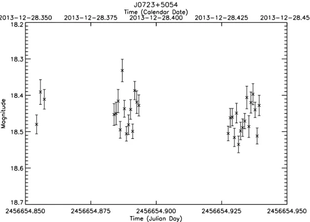
3.7 J0723+5054 . . . 50

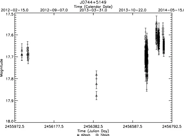
3.8 J0744+5149 . . . 52

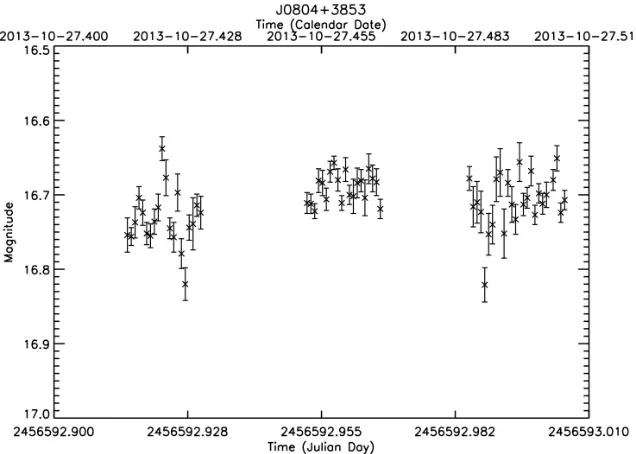
3.9 J0804+3853 . . . 53

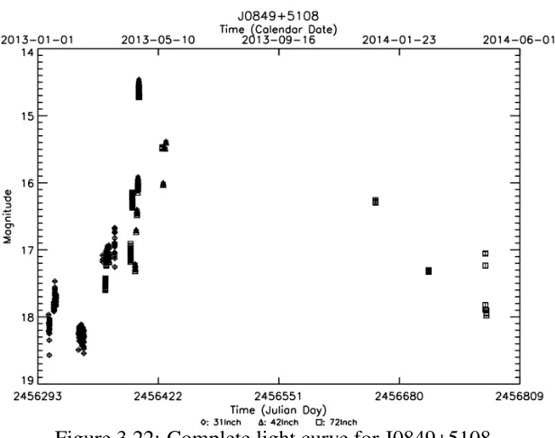
3.10 J0849+5108 . . . 55

3.10.1 J0849+5108: Multi-Wavelength Light Curve . . . 56

3.10.2 J0849+5108: Spectral Energy Distribution . . . 61

3.11 IRAS 09426+1926 . . . 64

3.12 J0956+2515 . . . 65

3.13 J1038+4227 . . . 66

3.14 J1047+4725 . . . 68

3.15 J1102+2239 . . . 69

3.16 J1140+4622 . . . 71

3.17 J1146+3236 . . . 73

3.18 J1227+3214 . . . 74

3.19 J1246+0238 . . . 75

3.20 J1333+4141 . . . 77

3.21 J1358+2658 . . . 78

3.22 J1405+2657 . . . 80

3.23 J1421+2824 . . . 81

3.24 J1435+3132 . . . 82

(11)

3.26 PKS 1502+036 . . . 84

3.27 RX 1629+4007 . . . 86

3.28 J1633+4718 . . . 88

3.29 J1644+2619 . . . 90

3.30 B3 1702+457 . . . 91

3.31 J1709+2348 . . . 93

3.32 J1713+3523 . . . 95

3.33 IRAS 20181-2244 . . . 96

3.34 J2314+2243 . . . 98

3.35 Null Detections . . . 100

4 Results 105 4.1 Behavior of the Sample . . . 105

4.2 Individual Objects . . . 109

4.2.1 J0948+0022. . . 109

4.2.2 J0849+5108. . . 111

4.3 Amplitude of Microvariability . . . 113

4.4 g-Ray Loud vs.g-Ray Quiet Radio-Loud NLSy1s . . . 117

5 Conclusions 120 5.1 Determination of Blazar-Like Status . . . 120

5.2 Summary and Future Work . . . 124

(12)

A.2 J0153+2609 (IRAS 01506+2554) . . . 150

A.3 1H 0323+342 . . . 155

A.4 J0706+3901 . . . 160

A.5 J0723+5054 . . . 167

A.6 J0744+5149 . . . 170

A.7 J0804+3853 . . . 173

A.8 J0849+5108 . . . 177

A.9 IRAS 09426+1929 . . . 191

A.10 J0948+0022 . . . 195

A.11 J0956+2515 . . . 219

A.12 J1038+4227 . . . 222

A.13 J1047+4725 . . . 225

A.14 J1102+2239 . . . 228

A.15 J1140+4622 . . . 232

A.16 J1146+3236 . . . 236

A.17 J1227+3214 . . . 239

A.18 J1246+0238 . . . 242

A.19 J1333+4141 . . . 249

A.20 J1358+2658 . . . 252

A.21 J1405+2657 . . . 256

A.22 J1421+2824 . . . 260

A.23 J1435+3132 . . . 263

A.24 J1443+4725 . . . 268

A.25 PKS 1502+036 . . . 271

A.26 RX 16290+4007 . . . 276

A.27 J1633+4718 . . . 281

(13)

A.29 B3 1702+457 . . . 294

A.30 J1709+2348 . . . 299

A.31 J1713+3523 . . . 302

A.32 IRAS 20181-2244 . . . 306

A.33 J2314+2243 . . . 313

B Analysis Software 317 B.1 LCGen - Main Script . . . 317

B.2 LCGen - Input (Subscript) . . . 349

B.3 LCGen - Multi (Subscript) . . . 354

B.4 LCGen - Names (Subscript) . . . 382

B.5 LCGen - Plot (Subscript) . . . 391

B.6 LCGen - Object List . . . 403

(14)

List of Tables

1.1 Sample List . . . 17

2.1 Telescope Parameters . . . 20

2.2 Summary of Optical Data by Telescope . . . 21

2.3 Variability of Various Types of AGN . . . 27

3.1 Summary of Optical Variability Observations . . . 36

5.1 Objects that do not display blazar-like characteristics . . . 121

5.2 g-Ray Quiet Objects with Indeterminate Properties . . . 122

5.3 g-Ray Loud Objects with Indeterminate Properties . . . 123

5.4 Objects with Blazar-Like Properties . . . 124

5.5 Potentially Blazar-Like Objects . . . 125

A.1 Comparison stars for the field of J0100-0200 . . . 145

A.2 Optical Data for J0100-0200 . . . 146

A.3 Comparison stars for the field of IRAS 01506+2554 . . . 150

A.4 Optical Data for IRAS 01506+2554 . . . 151

A.5 Comparison stars for the field of 1H 0323+342 . . . 155

A.6 Optical Data for 1H 0323+342 . . . 156

A.7 Comparison stars for the field of J0706+3901 . . . 160

A.8 Optical Data for J0706+3901 . . . 161

(15)

A.17 Comparison stars for the field of IRAS 09426+1929 . . . 191

A.18 Optical Data for IRAS 09426+1929 . . . 192

(16)

A.49 Comparison stars for the field of PKS 1502+036 . . . 271

A.50 Optical Data for PKS 1502+036 . . . 272

A.51 Comparison stars for the field of RX 16290+4007 . . . 276

A.52 Optical Data for RX1629+4007 . . . 277

A.57 Comparison stars for the field of B3 1702+457 . . . 294

A.58 Optical Data for B3 1702+457 . . . 295

(17)

(18)

List of Figures

1.1 The unified model of AGN . . . 4

1.2 The spectra of various types of AGN . . . 6

1.3 Microvariability in a blazar . . . 7

1.4 Long term light curve of MKN 421 . . . 9

1.5 Generic SEDs of two blazars . . . 10

1.6 Multi-wavelength study of a blazar . . . 11

1.7 The gamma-ray sky as seen by Fermi . . . 14

1.8 SED of J0948+0022 . . . 15

2.1 Example Finding Chart . . . 23

2.2 GUI for the CCDPhot program . . . 24

2.3 GUI for the LCGen program . . . 26

2.4 Microvariability with poorly sampled data . . . 28

2.5 KS-Test for J0849+5108 observations . . . 32

2.6 Example OVRO Data . . . 33

3.1 SED of J0948+0022 . . . 39

3.2 Complete light curve for J0948+0022. . . 40

3.3 Activity of J0948+0022 at various brightnesses. . . 41

3.4 Microvariability structure for J0948+0022 . . . 42

3.5 Microvariability structure for J0948+0022 . . . 42

(19)

3.7 Daily light curve for J0100-0200. . . 44

3.8 Complete light curve for IRAS 01506+2554. . . 45

3.9 Daily light curve for IRAS 01506+2554. . . 45

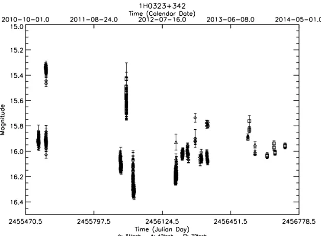
3.10 Complete light curve for 1H 0323+342. . . 47

3.11 Daily light curve for 1H 0323+342. . . 47

3.12 Morphology of 1H 0323+342 . . . 48

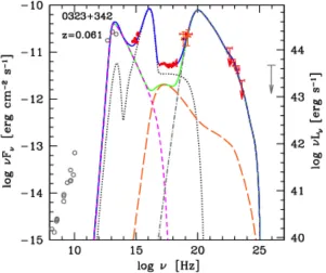
3.13 Spectral Energy Distribution of 1H 0323+342 . . . 48

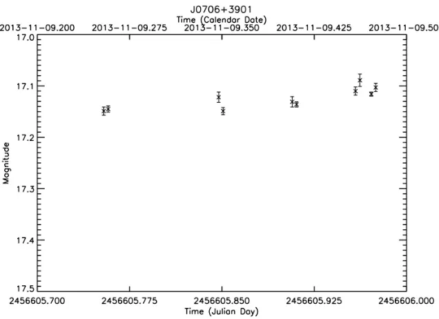
3.15 Daily light curve for J0706+3901. . . 50

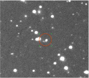
3.16 Morphology of J0723+3901 . . . 51

3.23 The optical andg-ray behavior of the object during the April flare event. . . 57

3.24 Microvariability structure for J0849+5108. . . 58

3.25 Microvariability during bright/faint states for J0849+5108 . . . 59

3.26 Multi-wavelength light curve of J0849+5108 . . . 60

3.27 SEDs of J0849+5108 . . . 62

3.28 Complete light curve for IRAS 09426+1929. . . 64

(20)

3.34 Morphology of J1102+2239 . . . 69

3.36 Daily light curve for 1102+2239. . . 70

3.35 Complete light curve for 1102+2239. . . 70

3.39 Morphology of J1146+3236 . . . 72

3.54 Spectral Energy Distribution of PKS 1502+036 . . . 85

3.55 Complete light curve for PKS 1502+036. . . 85

3.56 Daily light curve for PKS 1502+036. . . 86

3.57 Complete light curve for RX1629+4007. . . 87

3.58 Daily light curve for RX1629+4007. . . 87

3.59 Morphology of J1633+4718 . . . 88

(21)

3.65 Complete light curve for B3 1702+457. . . 92

3.64 Morphology of B3 1702+457 . . . 92

3.66 Daily light curve for B3 1702+457. . . 93

3.71 Morphology of IRAS 20181-2244 . . . 97

3.72 Complete light curve for IRAS 20181-2244. . . 97

3.73 Daily light curve for IRAS 20181-2244. . . 98

3.76 Daily light curve for B3 1702+457. . . 100

3.77 Daily light curve for 1H 0323+342. . . 101

3.79 Daily light curve for IRAS 09426+1926. . . 102

4.1 Amplitude of Variability vs. Duty Cycle . . . 106

4.2 Microvariability vs Duty Cycle . . . 107

(22)

4.5 Number of Microvarying Events vs. Amplitude of Events (Blazars) . . . 115 4.6 KS-Test of the radio-loud NLSy1, LBL, and HBL Populations . . . 116 4.7 Distribution of Duty Cycles in the Sample . . . 118

(23)

(24)

(25)

(26)

(27)

(28)

(29)

(30)

Chapter 1 Introduction

The field of active galactic nuclei (AGN) has enjoyed enormous success in uniting an array of seemingly disparate observed phenomena under a single conceptual framework. All AGNs are now thought to consist of otherwise normal galaxies that host an accreting super-massive black hole (SMBH) in their cores. This black hole is surrounded by a thick torus of hot gas and dust; the observed differences between the various sub-types of AGN, from the closest Seyfert galaxies to the most distant quasars, are now assumed to primarily be a simple consequence of the angle at which the observer is viewing the central environment of the SMBH relative to this obscuring torus. In radio-loud AGN, a collimated jet of plasma ejected at relativistic speeds perpendicular to the plane of the accretion disk is added to this scenario.

(31)

become aware of a potential new class of AGN with properties shared by both Seyfert galaxies and blazars. This study will attempt to add to the growing body of evidence for the existence of this new class and describe the observed properties of the objects that represent it.

1.1 An Overview of Active Galactic Nuclei

Prior to the 1900s, it was unknown if so-called “spiral nebula” were objects residing within our own galaxy or were distinct from the Milky Way. This debate was eventually settled by the Cepheid variable observations of Edwin Hubble in the 1920’s, finally opening the field of extragalactic astronomy as a major area of study (Hubble, 1925). Work in the early half of the 20th century then focused on describing the characteristics of these objects; most notable to this discussion was the revelation that a subset of spiral galaxies demonstrated spectra with nuclear emission lines (Hubble, 1926), in what was to become the first major hint as to the existence of active galactic nuclei. This period of astronomy culminated in the work of Carl Seyfert in 1943, which offered the first systematic study of the galaxies that now bear his name (Seyfert, 1943). Though the work of Seyfert was critical in offering a first description of the properties of AGNs, it was not until the advent of radio astronomy that research into active galaxies truly took off.

After the conclusion of the second world war in 1945, radio engineers seeking employment of their skills during peacetime turned to the field of astronomy, swiftly identifying now-famous radio galaxies such as Cygnus A. Optical identification of these sources followed some years later. One astronomer engaged in this effort was Allan Sandage, who in 1960 delivered an unscheduled paper1_{to the December meeting of the American Astronomical Society detailing his observations}

of the radio galaxy 3C 48 (Matthews et al., 1961) . Sandage reported the existence of an optical star-like object located at the coordinates of the radio galaxy. This object proved to be variable and possessed an excess of UV emission when compared to normal stars, but its most noticeable feature was spectroscopic — emission lines that were both broadened and located at wavelengths never before seen. Sandage maintained that the object was nevertheless most likely a star within our

1_{Because it was off-schedule this paper was never published, though it was later summarized in the magazine}_Sky

(32)

own galaxy that happened to lie along the same line of sight. This explanation eventually began to strain the concept of plausibility as the optical counterparts to an increasingly large number of radio galaxies were discovered with similar star-like objects “superimposed” on them. These galaxies have since come to be known as Quasi-Stellar Radio Objects (QSOs), or alternatively “quasars”.

In 1963, Maarten Schmidt realized that the previously inexplicable emission lines of a second quasar, 3C 273, were in actuality nothing more exotic than the hydrogen Balmer series. The reason these lines had not been immediately recognizable was due to a large redshift (z = 0.16, fairly unremarkable by today’s standards but unexpected at the time), which had moved them to unexpected locations. A reexamination of the spectrum of 3C 48 revealed that the previously baffling emission lines were also simply due to redshifting, albeit at a higher degree. Schmidt and the colleagues who had collaborated with him quickly published these results in a series of 4 related papers inNature(Schmidt, 1963; Hazard et al., 1963; Greenstein, 1963; Oke, 1963).

It was now apparent that quasars were not near-by objects, but rather were hosted within the radio galaxies with which they were associated. Given the distances implied by the measured redshifts and the apparent magnitudes at which they were observed, quasars had to be significantly brighter than even the brightest known galaxies, yet the emitting region was less than a kiloparsec in diameter. An object of previously unimaginable power was obviously present in the hearts of these galaxies.

(33)

[image:33.612.162.449.71.431.2]

Figure 1.1: The unified model of AGN Credit: Urry and Padovani (1995)

(34)

In addition to the black hole, disk, and jet (if present), an AGN is also thought to be surrounded by clouds of gas divided into two distinct regions. The inner-most area is known as the Broad-Line Region (BLR), so called because emission lines detected from this environment are broadened due to the high velocity of gas close to the black hole. The second area is called the Narrow-Line Region (NLR) for the opposite reason; being further away from the black hole, emitting gas has a lower velocity and therefore the spectral lines are less broadened. The final component of the standard model consists of a thick, obscuring torus of gas and dust that lies in the same plane as the accretion disk, surrounding it but also extending a significant distance both above and below it. It should be noted, however, that it is difficult to explain how this torus can retain its structure without flattening out into an extension of the disk. An alternative explanation consists of outflows of gas and dust blasted off the edges of the accretion disk by hydromagnetic winds (Emmering et al., 1992). The entire system is at most a few parsecs in radius and is likely smaller, roughly comparable in size to our own solar system (although the NLR can extend significantly further, on the order of hundreds of parsecs).

(35)

Figure 1.2: The spectra of various types of AGN

This figure was obtained from the personal website of Bill Keel at the University of Alabama at the following URL: http://www.astr.ua.edu/keel/agn/spectra.html. Of particular note is the presence of both broad and narrow emission lines in Seyfert 1 galaxies and BLRGs, whereas only narrow lines are detected in Seyfert 2 galaxies and NLRGs.

1.2 Blazars: an extreme class of AGN

Blazars represent a specific case of radio-loud AGN where the relativistic jets happens to lie al-most directly along the line of sight. This unique orientation produces relativistic beaming effects whereby light is preferentially emitted along the direction of motion and therefore enhances the perceived brightness of the jet headed toward the observer while dimming the jet headed away. Thus, it is common to detect only one jet when viewing a blazar.

(36)

Figure 1.3: Microvariability in a blazar

Rapid optical variability seen within a single night of observation for the blazar 0716+714. This figure was taken from Pollock et al. (2007).

first class, BL Lac objects, are defined as having featureless spectra, although very weak lines can sometimes be seen when an object is in a faint state. Refer back to Figure 1.2 for an example of this sort of spectrum. BL Lac objects can be contrasted with Optically Violent Variable (OVV) sources, also commonly called Flat Spectrum Radio Quasars (FSRQs), which have strong emission lines. FSRQs are dominated by (but do not completely overlap with) a third group known as Low energy peaked BL Lac objects (LBLs), which as a class are contrasted with High energy peaked BL Lacs (HBLs). The differences between HBLs and LBLs will be more throughly explored in section 1.2.2.

1.2.1 Variability

(37)

down to the order of a few hours or less. In fact, BL Lacertae itself, the object from which an entire class of blazars derive its name, was first mistaken for a variable star until it was eventually identified as an extragalactic radio source (Schmitt, 1968). Variability on these extremely rapid time scales is often referred to as “intranight” variability or (as will be the case for the remainder of this document) microvariability, terms that were coined in Wagner and Witzel (1995) and Miller et al. (1989) respectively. An example of such rapid variability can be seen in Figure 1.3

As an aside, it should be noted that the existence of microvariability in blazars was originally discounted. Evidence of the phenomenon was seen in the very earliest studies of quasars (Matthews and Sandage, 1963), but many astronomers attributed these observations to atmospheric effects rather than any processes intrinsic to the source. However, several decades of monitoring numerous blazars eventually supported the reality of this behavior (Miller et al., 1974; Miller, 1988; Carini et al., 1990, 1991).

In addition to being extremely rapid, the variability of blazars is also of remarkably high am-plitude. The very term “blazar” reflects this fact, having been invented by Edward Spiegel during a 1978 banquet speech in reference to their violent, “blazing” nature (Angel and Stockman, 1980). It is not unheard of for blazars (particularly LBLs) to vary by more than a magnitude within a single night of observation. On larger time scales of months or years, blazars can vary by as much as 5 magnitudes or more, as seen in the decadal behavior of the blazar Markarian 421 in Figure 1.4. In recent years, blazars have been subjected to world-wide, intensive monitoring campaigns such as the Whole Earth Blazar Telescope (WEBT) or the GLAST-AGILE Support Program (GASP), providing essentially continuous, intensive monitoring of selected sources (Mattox, 1998; Raiteri and Villata, 2008).

(38)

1975ApJ...201L.109M

Figure 1.4: Long term light curve of MKN 421

This figure is reprinted from Miller (1975). Data was obtained from Harvard College Observatory’s archival plates. Magnitudes are in the optical B band.

1.2.2 Multi-wavelength Behavior

(39)

Figure 1.5: Generic SEDs of two blazars

This figure was obtained from the following URL: http://physics.gmu.edu/~rms/blazars/

emitted from the jets themselves. Therefore, a reader will often find the phrases “self-Compton up-scattering” or (more commonly) “Synchrotron Self-Compton” used in reference to this peak in the literature. It should also be noted that due to the highly variable nature of blazar emission, the shape of the SED particular to any individual object is subject to change; both the amplitude and peak frequencies of the SED can shift during major flare events (Villata et al., 2006), although not to the extent of transforming an LBL-type object into an HBL (or vice versa).

(40)

Figure 1.6: Multi-wavelength study of a blazar

(41)

of a shock front forming in the inner regions of the AGN and traveling down the jet. Thus, by ob-serving a blazar across the electromagnetic spectrum and looking for correlations or lags between bands it is possible to infer details about the physical structure of the emitting region.

However, as previously stated, blazars will often not show any detectable correlations. In-deed, individual objects have been known to show correlations at certain epochs or time scales, but follow-up observations may find no sign of them. Examples of both correlated and non-correlated emission can be seen in Figure 1.6. Understanding the multi-wavelength variability is a subject of on-going research, although there are some indications that different wavelengths become increas-ingly correlated when a given blazar is at a higher flux state (Osterman et al., 2007).

1.2.3 Polarization

At lower energies blazars are often highly polarized, particularly in the optical and radio regimes. During flare states, blazars have been known to reach optical polarizations on the order of 30% (Tinbergen, 1996). This polarization is a consequence of the magnetic fields responsible for gen-erating the synchrotron emission from the jet that peaks in this energy range. Therefore, by inves-tigating changes in the polarized behavior of blazars astronomers gain a direct method of probing the structure of the jet itself.

Polarization values for objects of interest will be compared to values observed for blazars as a class, but no further study will be attempted. If the reader is interested in the polarized behavior of blazars and similar objects, they are encouraged to read the dissertation of Joseph Eggen, which was prepared in collaboration with (and in many respects serves as a companion to) this investigation (Eggen, 2014a).

1.3 Very Radio-Loud Narrow-Line Seyfert 1 Galaxies

(42)

Goodrich, 1989). A third criterion, the presence of FeII emission, is often included but is not part of the formal definition. The “narrow-line” component of their names is derived from the fact that in these objects the broad line region fails to live up to its name, producing the least broadened Balmer lines of any AGN. Physically, this is often taken to indicate that NLSy1s host relatively low-mass SMBHs. Interestingly, and despite their small sizes, the black holes of NLSy1s appear to be accreting at or near the Eddington rate (Boroson and Green, 1992). An alternative explanation — and one that will be of particular significance to this paper — is that NLSy1s are viewed at a near face-on viewing angle. In this scenario, the bulk motion of the BLR is nearly tangential to the line of sight, and therefore only weakly redshifted or blueshifted.

In 1989 the NLSy1 PKS 0558-504 became the first object of its class to be classified as radio-loud (Remillard et al., 1989). As similar narrow-line Seyfert galaxies were gradually discovered over the years this has proved to be unusual; most (93%) of NLSy1s are radio quiet, formally defined as having a radio loudness parameter R < 10, where R is the ratio between the observed flux in the 5 GHz radio band compared to the optical B band (Komossa et al., 2006). Even where radio loudness is detected, most NLSy1s tend to barely qualify, with a mere 2.5% reaching the R > 100 threshold for very radio loud objects. It would therefore seem that relativistic jets are a rarity among NLSy1s, and are comparatively weak when present.

The Compton Gamma-Ray Observatory (CGRO) was launched in 1991, and equipped with the EGRET instrument this telescope was able to conduct the first all-sky survey in the gamma-ray regime, revealing a number of variable extragalactic sources. In 2008, CGRO was succeeded by the more sophisticated Gamma-Ray Large Area Space Telescope (GLAST), later renamed the Fermi Space Telescope in honor of Enrico Fermi. The principle instrument on board Fermi is the Large Area Telescope (LAT), capable of detecting photons with energies up to ~300 GeV (ten times higher than EGRET) and boasting a field of view equal to 2.4 steradians2 _{(Atwood et al.,}

2009).

As can be seen in Figure 1.7, active galaxies are by far the most prominent class of objects in

(43)

Figure 1.7: The gamma-ray sky as seen by Fermi

the gamma-ray sky, with the overwhelming majority of known objects identified as blazars. Only 1% of the sources detected by Fermi are non-blazar AGNs, but these are the objects that will be of particular interest to this paper. Within months of first light, Fermi detected gamma-ray emission from a highly unusual object with the designation J0948+0022. A multi-wavelength campaign swiftly ensued and discovered that the object possessed the classic double-peaked SED indicative of a blazar (Abdo et al., 2009a). As seen in Figure 1.8, the SED closely resembled that of an LBL. At the same time, J0948+0022 demonstrated a FWHM Hb⇡1500 km/s and weak forbidden lines,

indicative of a NLSy1. Confusing the issue still further, the object was found to be very radio loud, having a radio loudness of log(R) = 2.93. By the end of the year, three more such objects had been identified, leading to the possibility of the existence of a new class of gamma-ray loud AGN, the very radio-loud narrow-line Seyfert 1 galaxies (Abdo et al., 2009b).

(44)

gamma-0 0 1 0 1 1 frequency [GHz] 0.25 0.5

flux density [Jy]

January 24, 2009

Figure 3. Evolution of the radio spectrum of PMN J0948+022. Filled circles denote the Effelsberg observations of 2009 January. Archival data are shown in gray: triangles represent VLBA measurements conducted in 2003 October (Doi et al.2006) and diamonds represent archival Effelsberg measurements obtained in 2006 (Vollmer et al.2008).

3.3. Radio

3.3.1. Effelsberg

The centimeter spectrum of PMN J0948+0022 was observed

with the Effelsberg 100 m telescope on 2009 January 24 (MJD

54855.5) within the framework of a

Fermi

-related

monitor-ing program of potential

γ

-ray blazars (F-GAMMA project;

Fuhrmann et al.

2007

). The measurements were conducted with

the secondary focus heterodyne receivers at 2.64, 4.85, 8.35,

10.45, 14.60, and 32.00 GHz. The observations were performed

quasi-simultaneously with cross-scans, that is, slewing over the

source position, in azimuth and elevation directions, with

adap-tive numbers of sub-scans for reaching the desired sensitivity

(for details, see Fuhrmann et al.

2008

; Angelakis et al.

2008

).

Pointing offset correction, gain correction, atmospheric opacity

correction, and sensitivity correction have been applied to the

data.

The radio spectrum acquired has a convex shape with a

turnover frequency between 10.45 and 14.60 GHz (Figure

3 ).

The low-frequency part spectral index

α

₂10_.₆₄.45

, measured between

2.64 and 10.45 GHz, is

₋

0 .

18 ±

0 .

02, whereas the

high-frequency optically thin spectral index

α

₁₄32_.₆

₌

0 .

39. The comparison of the acquired spectrum with previously

observed ones (Vollmer et al.

2008

; Doi et al.

2006

) reveals

that the source is presently in a much lower flux density state

(see Figure

3 ). This indicates intense variability. From the

change of the 4.85 GHz flux density over about three years

(Vollmer et al.

2008

), we estimate a variability brightness

temperature (e.g., Fuhrmann et al.

2008

) of 1

.

4 ×

10

11

K. Assuming the equipartition brightness temperature limit of

∼

10

11

K (Readhead

1994

), we obtain a lower limit for the

Doppler factor of

δ

>

1 .

4. 3.3.2. Owens Valley Radio Observatory

PMN J0948+0022 has been regularly observed from 2007

September 4 at 16:25 UTC to 2009 February 11 at 06:53 UTC

(MJD 54347.68

₋

54873.29) at 15 GHz by the OVRO 40 m

telescope as part of an ongoing

Fermi

blazar monitoring program

of all 1159 Candidate Gamma-Ray Blazar Survey (CGRaBS)

blazars north of decl.

₋

20

◦

_{(Healey et al.}

₂₀₀₈

_{). Flux densities}

were measured using azimuth double switching as described in

Readhead et al. (

1989

). The relative uncertainties in flux density

Figure 4. SED of PMN J0948+0022.Fermi/LAT (five months of data), Swift XRT and UVOT (2008 December 5), Effelsberg (2009 January 24) and OVRO (average in the five months of LAT data, indicated with a red diamond) are indicated with red symbols. Archival data are marked with green symbols. Radio data: from 1.4 to 15 GHz from Bennett et al. (1986), Becker et al. (1991), Gregory & Condon (1991), White & Becker (1992), Griffith et al. (1995), and Doi et al. (2006). Optical/IR: USNO B1,B,R,Ifilters (Monet et al. 2003); 2MASSJ, H,Kfilters (Cutri et al.2003). The dotted line indicates the contributions from the infrared torus, the accretion disk, and the X-ray corona. The synchrotron (self-absorbed) is shown with a small dashed line. The SSC and EC components are displayed with dashed and dot-dashed lines, respectively. The continuous line indicates the sum of all the contributions.

(A color version of this figure is available in the online journal.)

result from a 5 mJy typical thermal uncertainty in quadrature

with a 1.6% systematic uncertainty. The absolute flux density

scale is calibrated to about 5% using the model for 3C 286 by

Baars et al. (

1977

). This absolute uncertainty is not included in

the plotted errors.

PMN J0948+0022 has been reported to show variability by

a factor of 2 in radio over year timescales (Zhou et al.

2003

)

and

_∼

31% fluctuations in month timescales (Doi et al.

2006

).

The OVRO 40 m 15 GHz time series shows a clear structure at

timescales down to weeks and year-scale fluctuations by a factor

of 4 (Figure

2 , panel (C)). The rapid variability we observe in

this object—at least 400 mJy in 77 days or 5 mJy

/

day—enables

us to determine a variability brightness temperature of

_∼

2 _×

10

13

K, assuming the

Λ

CDM cosmology described in Section

1 .

It is often not easy to determine the optically thin spectral

index of blazars at radio frequencies because they are complex

structures, with different regions becoming optically thin at

different radio frequencies. In the present case, the most recent

results show a turnover between 10 and 15 GHz, and a 15–

30 GHz spectral index of

_∼

0 .

4, but we do not believe that this

is the optically thin spectral index. It is much more likely that

one still sees synchrotron self-absorption so that the spectrum

between 15 GHz and 30 GHz is much flatter than the true

optically thin spectral index. In such cases, it is safer to assume

an optically thin spectral index of 0

.

75 and to use the frequency

of observation. These only have a small effect on the derived

T

eq

unless

α

is very close to 0

.

5, which is too flat, in our view,

for an optically thin spectral index in most cases.

The equipartition brightness temperature (Readhead

1994

),

in the current cosmological model, is then

T

eq

∼

5 .

5 ×

10

K,

assuming an average optically thin spectral index of 0

.

75, and

hence the equipartition Doppler factor is

δ

∼

7, which is typical

Figure 1.8: SED of J0948+0022

This figure first appeared in Abdo et al. (2009a). Note the double peak structure of the actual data (not the modeling), and how similar it is to Figure 1.5.

ray emission). They are distinct from blazars in that the morphology of their host galaxies have empirically been found to be spirals, whereas the host galaxies of blazars have been observed to be elliptical galaxies3 (Urry et al., 2000). Radio-loud NLSy1s may therefore be the previously “missing” blazar population associated with spiral galaxies.

1.4 Synopsis of Dissertation

The case for very radio-loud NLSy1s being blazar-like AGN is a strong one. However, not all aspects of blazar behavior have yet to be investigated in this new class. Most notably, there have been few reported attempts to detect the short-term, intranight variations that are commonly seen among blazars. Of those investigations that do exist, all of them focus on individual sources rather

(45)

than the class as a whole. The lack of any such systematic analysis is perhaps understandable; many of the currently known radio-loud NLSy1s are unfortunately faint, and detections of mi-crovariability necessitate the dedication of a great deal of observing time. This thesis will provide such a systematic study of this class of AGN.

A sample of approximately three dozen radio-loud NLSy1 galaxies has been assembled to test for the existence of microvariability. These objects have been selected from the sample of Yuan et al. (2008), choosing only those objects with R 100. Additional radio-loud NLSy1s (including those at lower R values) were obtained from Komossa et al. (2006) and Whalen et al. (2006). The full sample of objects that will be used in this investigation can be seen in Table 1.1.

(46)

Table 1.1: Sample List

Columns are: (1) name of the object, (2) right ascension (2000), (3) declination (2000), (4) redshift, (5) radio loudness, (6) Test Statistic values forg-ray detections,

and (7)g-ray loudness (Definitions of TS and log(G) are found in section 2.2)

Object R.A. Dec. z log(R) TS log(g)

J0100-0200 01 00 32.22 -02 00 46.00 0.227 1.77 9.65 6.27

IRAS 01506+2554 01 53 28.30 +26 09 40.00 0.326 1.40 –

1H 0323+342 03 24 41.16 +34 10 45.86 0.063 2.50 280.31 6.81

J0706+3901 07 06 25.12 +39 01 51.55 0.086 1.21 10.50 7.79

J0723+5054 07 23 02.33 +50 54 48.00 0.203 1.29 – –

J0744+5149 07 44 02.28 +51 49 17.50 0.460 1.62 – –

J0804+3853 08 04 09.24 +38 53 48.83 0.211 1.18 10.77 7.06

J0849+5108 08 49 57.98 +51 08 29.02 0.583 3.16 790.76 7.33

IRAS 09426+1926 09 45 29.22 +19 15 48.70 0.284 1.56 – –

J0948+0022 09 48 57.32 +00 22 25.51 0.584 2.93 402.14 6.09

J0956+2515 09 56 49.87 +25 15 16.20 0.712 3.56 95.95 6.48

J1038+4227 10 38 59.58 +42 27 42.21 0.220 1.30 – –

J1047+4725 10 47 32.69 +47 25 32.01 0.800 4.09 – –

J1102+2239 11 02 23.38 +22 39 20.69 0.453 1.28 14.57 6.96

J1140+4622 11 40 47.90 +46 22 04.79 0.115 1.36 – –

J1146+3236 11 46 54.29 +32 36 52.38 0.465 2.19 12.61 6.88

J1227+3214 12 27 49.14 +32 14 59.00 0.137 1.36 – –

J1246+0238 12 46 50.20 +02 40 16.00 0.091 2.38 17.13 7.74

J1333+4141 13 33 45.47 +41 41 27.66 0.225 1.06 – –

J1358+2658 13 58 45.37 +26 58 08.48 0.330 1.11 – –

(47)

Table 1.1 cont.

J1421+2824 14 21 14.06 +28 24 52.90 0.538 2.14 – –

J1435+3132 14 35 09.50 +31 31 47.97 0.502 2.98 – –

J1443+4725 14 43 18.56 +47 25 56.66 0.703 3.03 27.81 7.25

PKS 1502+036 15 05 06.48 +03 26 30.80 0.411 3.53 36.60 5.81

RX 16290+4007 16 29 01.31 +40 07 59.94 0.272 1.61 – –

J1633+4718 16 33 23.57 +47 18 58.83 0.116 2.19 – –

J1644+2619 16 44 42.53 +26 19 13.30 0.145 2.73 52.25 7.01

B3 1702+457 17 03 30.41 +45 40 47.08 0.061 2.01 – –

J1709+2348 17 09 07.81 +23 48 37.76 0.254 1.06 – –

J1713+3523 17 13 04.46 +35 23 33.65 0.083 1.05 12.03 7.08

IRAS 20181-2244 20 21 04.40 -22 35 18.00 0.185 1.57 9.42 6.89

(48)

Chapter 2 Data Processing

The data used in this work were obtained from a variety of telescopes working at several wave-lengths. Although the bulk of the data were obtained from Lowell Observatory, other sources include the Owens Valley Radio Observatory (OVRO), the Cerro Tololo Inter-American Observa-tory (CTIO), and NASA’s Fermi-LAT space telescope; a summary of the basic characteristics of these instruments can be found in Table 2.1 on the following page. While data from some of these instruments were provided pre-reduced, others required significant processing before their results could be compared to other sources. Further, some basic information about individual objects such as redshift or radio loudness was obtained from the literature. With data being obtained from such disparate sources, care had to be taken to ensure that the results reported in this document were both consistent and reliable.

2.1 Optical Data

(49)

approx-Table 2.1: Telescope Parameters

Telescope Observatory Bandpass Detector Field of View

40m OVRO 15 GHZ —— 157” radius

SMARTS 1.3m CTIO optical/IR ANDICAM 6.0’ x 6.0’

31” NURO Lowell optical NASAcam 15.6’ x 15.6’

42” Hall Lowell optical SITe 19.4’ x 19.4’

72” Perkins Lowell optical PRISM 13.6’ x 13.6’

Fermi-LAT space telescope 20 MeV-300 GeV —— 60º radius

Fields of view for the Lowell instruments assume 2x2 binning.

imately 6-day intervals (with a total range of 4-16 days) spaced roughly one month apart. Usually, observing windows were centered on the new moon. As it would have been unfeasible for an in-dividual graduate student to travel to Flagstaff once every lunar cycle, by mutual agreement I and fellow graduate student Joseph Eggen agreed to take alternate observing sessions. Whomever was at the telescope would then collect data for both of our respective projects. Therefore, it can be assumed that roughly half of the data from Lowell appearing in this document were obtained by each of us, with only minor contributions coming from additional observers.

Observations at Lowell related to this project began November 2010 and continued to be col-lected until April 2014. In that time span, 336 nights were allocated to our research projects across the three instruments. Photometry data was actually collected on 285 of these nights; the remain-der were either lost due to poor weather or were spent collecting data for Joseph Eggen’s project. The automated observing sessions on the 31” telescope frequently overlapped with those of the 42” and 72”; in these cases, the 31” was typically instructed to obtain observations of 5-10 objects while the human observer on the other telescope studied a second set of objects. A summary of the optical data obtained at Lowell can be found in Table 2.2.

(50)

ob-Table 2.2: Summary of Optical Data by Telescope (Number of allocated nights are in parentheses)

Telescope Observing Nights Observations

Whole Sample 285 11,920

Lowell 31” 80 (169) 3,903

Lowell 42” 57 (91) 3,678

Lowell 72” 68 (151) 4,183

SMARTS 1.3m 138 156

tained by on-site observers and uploaded to an online server; the data was then periodically down-loaded by members of the PEGA group to be used locally. The SMARTS telescope obtained data for the PEGA group approximately 3 out of every 4 nights from November 2010 to April 2014, for a total of 968 nights. However, in contrast to the Lowell instruments typically only 1-3 objects were observed each night, and so the SMARTS telescope was primarily used to keep track of on-going activity between the more focused observing sessions at Lowell. Furthermore, the bulk of the SMARTS data were not directly related to this project, consisting instead of on-going blazar monitoring as part of several long-term studies, largely due to the fact that only a few of the radio-loud NLSy1s in the sample could be seen from the southern latitude at which CTIO is located. In the end, only 14% of the SMARTS observations were used in this project, but this still accounted for 138 nights of data, as can be seen in Table 2.2.

2.1.1 Optical Data Reduction

(51)

read-out noise of the instrument. This noise is primarily caused by electronic sources, such as stray currents during the read-out process. Though ideally the bias-level noise will be uniform across the detector, imperfections in the structure of the chip will induce minor variations. By combining multiple bias frames into a single averaged master bias these variations are minimized, while at the same time removing the effects of transient sources such as cosmic rays.

In a similar manner, a set of ten flat fielding images were obtained at least once per observing session and then combined into an averaged master flat frame (although more typically flats were acquired on multiple nights and a master flat was created for each individual night). Flat fielding images help to improve the quality of science frames by removing the effects of nonconformity in pixel sensitivity, image distortions such as vignetting, and by accounting for obstructions in the optical path such as dust grains on the telescope lens. This is accomplished by acquiring an evenly illuminated, unfocused image using the same filter as the science data, either by aiming the telescope at a blank screen or the empty sky during twilight1. Under these circumstances any pixel to pixel variations will be entirely due to the previously mentioned effects, which can therefore be quantified and removed from the science images. By taking multiple flats and averaging them together transient effects are minimized or removed, as was the case with the bias frames.

No dark frames were obtained due to the fact that the CCD cameras of all three telescopes are cooled using liquid nitrogen to the point that dark current is considered negligible. Once the master bias and flat images had been created for an observing session, they were applied to the accompanying science frames using standard Image Reduction and Analysis Facility (IRAF) routines. First, the master bias file was subtracted from each object frame. Then the science images were divided by the master flat, resulting in object images cleansed of imperfections in the optical light path or the CCD electronics. Typically this process was automated using the “pegaproc” reduction script written by former graduate student John McFarland.

Data reduction for the SMARTS telescope was virtually identical to that of data taken at the

1_{It was decided that flat fielding images at Lowell would be acquired through the use of an in-dome screen rather}

(52)

Figure 2.1: Example Finding Chart

Finding Chart for the NLSy1 J0100-0200. The object is in the center of the field and is indicated by the vertical lines. Comparison stars are circled and numbered.

Lowell instruments, except that images were processed at CTIO before being retrieved by the PEGA group from their online servers. As a final note, all of the optical data used in this project were taken using a standard Johnson R band filter. This filter was chosen so as to be consistent with the archived observations of blazars and other AGN obtained by previous graduate students, the majority of which were also in the R band.

2.1.2 Optical Photometry

(53)

Figure 2.2: GUI for the CCDPhot program

course of the night will affect all objects equally, allowing for direct comparisons between them. This also allows for a more efficient use of telescope time, as science images effectively double as their own calibration frames.

(54)

location. The new positions of the previously defined comparison stars can then be automatically re-determined based on this new position. As each frame is processed the image is briefly displayed on the computer screen, allowing the user to track events such as passing clouds or satellites.

An aperture radius of seven arc-seconds was chosen when working with all of the data that appears in this document in order to assure consistency between differing objects and epochs; this also makes the data presented in this study consistent with the published blazar work from previous graduate students, ensuring ease of comparison between samples. The background level was determined from an annulus that was centered on each aperture, then subtracted from the measured values2_{. The instrumental magnitudes of the target and comparison stars were then}

calculated and the results written to an output file.

If (as assumed) the chosen comparison stars are non-varying sources then the relative differ-ences between their instrumental magnitudes will remain constant, as any transient effects having to do with the local atmosphere will affect all of them equally. The differential magnitude be-tween the comparison stars and the target, however, willnotbe constant if the target is of varying brightness. Therefore, the magnitude of the object of interest can be determined by comparing the brightness of each available field star to the target.

If the apparent magnitudes of the comparison stars are known, an offset between these values and their observed instrumental magnitudes can be found. Ideally, because all of the stars lie in the same image this offset should be identical for every object. Once found, the apparent magnitude of the target of interest can be determined by applying the same offset to it. This technique has the advantage of allowing measurements of the apparent magnitude of the object to be directly compared to results found during other nights or when using other instruments. The drawback is that the uncertainty of the measurement is increased, as one must now account for the spread in the instrumental/apparent magnitude offset and the uncertainties in the measurement of the brightness

2_{A minority of the objects in the sample have extended host galaxies that lie within this annulus and therefore}

(55)

Figure 2.3: GUI for the LCGen program

of the comparison stars.

(56)

Table 2.3: Variability of Various Types of AGN

Data were obtained from Miller and Noble (1996), Netzer et al. (1996), Ferrara (2000), Carini et al. (2003), Campbell (2004) and Goyal et al. (2013).

Approximate Approximate Maximum Amplitudes

Source Type Duty Cycle Microvariability Long-Term Variability

Radio Quiet NLSy1s 4% 4m~ 0.05 4m~1

Radio Quiet Quasars 10% 4m~ 0.10 4m~1

Radio-Loud Quasars 19% 4m~ 0.10 4m~1

HBL and TeV Blazars 45% 4m< 0.15 4m~ 2

LBL Blazars 80% 4m> 0.20 4m~ 3

individual objects: for example, it can be told (and later remember) that the names “BL Lac” and “PKS 2200+420” refer to the same object, and so it will find archived data registered under either name. All light curves that appear in this document were made through the use of LCGen. The IDL code for the script itself can be found in Appendix B.

2.1.3 Duty Cycles

Although more consistently active than other populations of AGN, blazars are only intermittently found in a microvarying state. This fact requires an additional parameter to be taken into account in order to accurately describe the relative variability of an object. For example, it two AGNs are found to have a maximum intra-night variability of 0.5 magnitudes then one might conclude they are similarly active. However, if one of the objects demonstrates these variations twice out of 10 nights while the other shows similar activity 7 out of 10 nights, then it is obvious that the latter object is more active than the former. Ideally, these observations would be spread over a significant range of time, as AGNs are known to periodically enter relatively active or quiescent states and this would allow such long-term trends to be averaged out.

(57)

Figure 2.4: Microvariability with poorly sampled data

During the gaps in the light curve, a second radio-loud NLSy1 was observed along with the pre-sented object on this night. Although this lowered the cadence at which either object was moni-tored, microvariability can still obviously be detected.

variability of various classes of AGN show distinct differences in both amplitude and duty cycle. For example, radio-quiet narrow-line Seyfert 1 galaxies demonstrate microvariations of no more than 0.05 magnitudes at a very low duty cycle of ~4%, based on observations of 14 objects over 72 nights of observation (Ferrara, 2000). This can be contrasted with LBL-type blazars, which possess typical duty cycles of ~80% and demonstrate variations four times larger (or more) in amplitude than what is seen in radio-quiet NLSy1s on similar time scales.

(58)

be observed in a 1-2-3-1-2-3 sequence for several hours. This naturally lowered the cadence at which any individual object was observed but increased the total number of objects for which data had been collected. While this likely prevented the observation of highly detailed structure within the variability, as can be seen in Figure 2.4 it still more than sufficed to allow a simple boolean statement as to whether or not an object was varying to be made.

Nights in which the microvariations were above a 3s standard deviation were treated as “con-firmed” nights of microvariability. However, many nights showed probable detections that fell between the 2.5s and 3s confidence thresholds. It was decided that these nights would be

in-cluded, but at half the weight of the confirmed nights3_{. Therefore, the duty cycles reported in this}

document were determined using the following simple equation:

DC= (Ncon f irmed+ 1

2Nprobable

NTotal )⇤100 (2.1)

whereNcon f irmed is the number of nights in which the object showed variations above the 3s level,

Nprobableis the number of nights in which the object showed variations between 2.5s and 3s, and

NTotal is the number of nights in which microvariability could have been observed (regardless of

whether or not it actually was).

2.1.4 Seyfert Finding Charts

Before differential photometry could be performed on the objects presented in this document, finding charts detailing in-field stars of known apparent magnitude were required. Multiple stars (typically 7, but ranging from 6-9) in each object field were selected for use in this analysis. These stars were chosen almost entirely at random, the only criteria for selection being that they were of comparable brightness to the radio loud NLSy1 under study (to within one or two magnitudes) and that they were isolated from other objects. Due to the admittedly non-rigorous method used to select them it was assumed that at least some of the stars would later prove to be variable sources;

3_{A weight of one half was chosen due to the fact that the uncertainty will vary by the square-root of the probability}

(59)

this is why so many were chosen for each field, as it allowed a few stars to be discarded should they prove to be untrustworthy. Each field was eventually left with at least two comparison stars known to be stable sources; otherwise, more stars would have been selected and investigated.

In order to find the apparent magnitudes of these stars the field around each object was observed during a photometric night and at nearly the same airmass (typically within a redshift of z=0.01) as several fields taken from the Landolt list of equatorial stars of known magnitude (Landolt, 1992). This allowed for a straightforward derivation of the non-instrumental apparent magnitude based on the observed magnitudes of the Landolt objects using an equation of the form

(mR,ob ject mR,Landolt)observed = (mR,ob ject mR,Landolt)apparent+kR(Xob ject XLandolt) (2.2)

wherem_R,ob jectrefers to the observed and apparent magnitudes of the in-field check star,mR,Landolt

refers to the observed and apparent magnitudes of a Landolt equatorial star, kR is the extinction

coefficient in the R band, and X refers to the airmass. Given the object and Landolt fields were observed at very nearly the same airmass, the last term of equation (2.2) is assumed to be essentially zero.

(60)

It has been reported that performing differential photometry using comparison stars that are sig-nificantly brighter than the object of interest (or vice versa) can lead to false detections of variability (Cellone et al., 2007). A comprehensive study of this effect by Goyal et al. (2013) determined that a dissimilarity of 1.5 magnitudes or less will not result in spurious detections, although this rep-resents a lower limit and greater differences may be permissible. Therefore, an active object that varied betweenmR= 13.0-18.0 would require check stars with brightnesses spanning at leastmR=

14.5-16.5 in order to insure the validity of any reported microvariability. Using this criterion, 31 of the 33 Seyfert galaxies presented in this document possess at least one field star of an appropriate luminosity at both the bright and faint extremes of its demonstrated variability.

Both of the exceptions involve objects that can become significantly fainter than the faintest available field star. The first, J1246+0238, only exceeds the 1.5-magnitude boundary by a further 0.3 magnitudes. Given that the value reported by Goyal et al. (2013) was intended to be a lower limit on the acceptable magnitude difference, this is probably only a minor concern. More seri-ous is the second case, that of J0849+5108, which when quiescent can be 2.7 magnitudes fainter than any of the comparison stars in its field. This is particularly troublesome given the fact that J0849+5108 is the most active object in the sample, and therefore of particular interest.

Of the 21 nights in which J0849+5108 was detected in a microvarying state, the object was bright enough to be within 1.5 magnitudes of at least one in-field comparison star on only 10 nights. In order to determine if the perceived variability from the remaining 11 nights was genuine, a Kolmogorov-Smirnov comparison (commonly known as the KS test) was performed on the two data sets. Specifically, the KS-test compared the amplitudes of the microvarying events when the object was in bright and faint states. The results can be seen in Figure 2.5. The KS-test found a D value of 0.26 and a corresponding P value indicating an 80% likelihood that the two populations were identical. Therefore, two of the 11 nights when the object was in a faint state are statistically likely to have been false detections of microvariability, leaving 19 probable or confirmed detections.

(61)

de-Figure 2.5: KS-Test for J0849+5108 observations

The red line indicates observations of microvariability during which the object was more than 1.5 magnitudes fainter than the faintest in-field check star. The blue line indicates observations during which the object was brighter than this value.

tections as “half nights” in determining the duty cycles for each object. In the case of J0849+5108, 4 of the 21 microvarying nights had detections between 2.5 and 3.0s. This implies a duty cycle of

(17con f irmed+(42)probable

21 )⇤100t90% . In turn, the KS-test would imply 19 / 21 nights were in a truly

microvarying state, or ~90%.

2.2 Other Wavelengths

The primary focus of this dissertation is the characterization of the optical variability of a sample of very radio-loud NLSY1 galaxies on timescales ranging from minutes to years. However, the nature of the sample is also evaluated based upon observations at other wavelengths, most notably the radio andg-ray regimes.

The radio-loudness parameter “R” – defined as R = f lux5GHz

f luxB ,the ratio between an object’s

(62)

Figure 2.6: Example OVRO Data

Radio data for the object J0849+5108 obtained from the Owens Valley Radio Telescope.

provided supporting radio observations for a small subset of objects in our sample. The OVRO program makes use of a 40-meter telescope and is designed to monitor a large sample of over 1600 AGNs in order to complement FERMI g-ray observations of these same objects (Richards et al., 2011). This data is made publicly available on their website.4 _{Repeated observations of the Seyfert}

galaxy 3C 286 are used in determining the absolute flux density of all objects observed under the monitoring program; this galaxy is both bright and known to be stable in brightness (Richards et al., 2011). For the purposes of calibration, 3C 286 is assumed to have a total flux density of 3.44 Jy (Baars et al., 1977) at an uncertainty of 5%. As of the time of this writing, three of the NLSy1s included in this study - J0849+5108, J0948+0022, and J0956+2515 - are included on the OVRO observing list. All three objects have been observed for nearly the full 6+ years the program has been in existence, having accumulated over 300 observations per object in that time. An example of this data can be seen in Figure 2.6.

The high energy data used in this dissertation were obtained from the public data server of the Fermi g-ray Space Telescope. The Large Area Telescope (LAT) on board Fermi is a pair-conversion detector sensitive to gamma rays in the 20MeV to several hundred GeV energy range (Atwood et al., 2009). The instrument has worked almost continuously in all-sky-mode since its

(63)

launch in June 2008, which allows coverage of the entire gamma ray sky approximately every 3 hours. The data were reduced and analyzed using ScienceTools v9r31p1 and instrument response functions P7SOURCE_V6. The likelihood analysis procedure as described at the FSSC website5

was used and the results of the analysis of the gamma ray detection (and the level at which those detections are significant) are taken from Eggen (2014b). These values are used both to establish which members of the sample are gamma-ray loud, and in the case of monitoring programs, to provide gamma-ray light curves for multi-wavelength monitoring of interesting and highly variable sources included in this sample.

A Test Statistic (TS) value is generally used when evaluating data from the Fermi Telescope for significance, where the square root of the TS value is approximately equal to the significance of detection for a given source. A TS value of 25 therefore corresponds to a 5-svdetection, whereas a value of 9 would indicate a 3-sv detection. In the literature, only those objects that have been detected at a TS value of 25 or more are considered “confirmed” gamma-ray sources. Formally, the Test Statistic is defined as TS = 2Dlog(likelihood), where likelihoodrefers to the likelihood ratio test as described in Mattox et al. (1996).

In addition to the TS value, theg-ray loudness parameter “G” will be used in this document as a means to gauge theg-ray loudness of an object. The G parameter is defined in Eggen (2014b) as G = f luxR

f lux₁GeV,the ratio between an object’s flux at the opticalRband and at 1 GeV. Not only is the g-ray loudness parameter more directly comparable to values of R for the radio regime, but like R

it has the advantage of being z-independent. This is due to the fact that both R and G are ratios of two flux values, each of which are equally affected by distance so that distance effectively cancels out.

(64)

Chapter 3 Observations and Object Activity

This chapter will briefly describe the data acquired for each object in the sample and will present analyses of selected sources; the full data set, which was quite large, can be found in Appendix A. As expected, several of the objects demonstrate behavior typical of a normal radio loud quasar, while others show dramatic activity that would be remarkable even for a known blazar. An analysis of these data will be presented in the following chapter.

3.1 The Sample

(65)

(66)

(67)

From the beginning of the project, it was expected that the sample would contain both blazar-like and more typically Seyfert-blazar-like galaxies, with the initial assumption being that those objects that demonstrated the greatest g-ray emission and/or radio loudness would also show the most blazar-like (i.e., frequent, rapid and high-amplitude) variability. As can be seen in Tables 1.1 and 3.1 , the reality – as is so often the case – is not so clearly defined. While the two objects most prominent in theg-ray regime (J0849+5108 and J0948+0022) do indeed also show the strongest microvarying behavior, the object with the next highest duty cycle (IRAS 20181-2244) is barely detectable in the g-rays. However, the third brightest g-ray object (1H 0323+342) exhibits very modest microvariability, demonstrating a duty cycle much lower than that of several objects com-pletely undetected at high energies. Attempts to distinguish between the blazar-like and Seyfert-like populations will be presented in chapter 4.

No systematic attempt to resolve the host galaxies of the objects in the sample was made. However, imaging1 revealed that at least seven of the objects were not grand design spirals. J0723+5054, J102+2239, J1633+2619, and IRAS 20181-2244 are interacting galaxies. 1H 0323+342 is a disrupted spiral with only one apparent arm, and a poorly resolved structure extends to the north of J1146+3236. B3 1102+457 is a barred spiral that may also be a ring galaxy. These objects are found at redshifts of up to z⇡0.45, and represent ~30% of the objects within that distance.

The following sections will present each object in the sample in order of increasing right as-cension, with the exception that the class prototype will be discussed first.

3.2 J0948+0022: The Class Prototype

J0948+0022 (2MASS J09485730+0022261) is the prototype for this new class of blazar-like ob-jects and was the first radio-loudNLSy1 discovered to emit in theg-ray regime. Subsequently it was extensively studied by Abdo et al. (2009a) and Foschini et al. (2010). As seen in Figure 3.1, the SED of the object demonstrates the classic double-peak structure of blazars (Abdo et al., 2009a). The object has also been observed to exhibit significant optical polarization (up to 15%), although

1_{These images were obtained from the Hubble space telescope in the case of 1H 0323+342 and from Lowell for}

(68)

Figure 3.1: SED of J0948+0022

This figure was taken from Abdo et al. (2009a).

(as is typical for blazars) this values changes rapidly (Eggen, 2014a). Figure 3.2 shows the light curve of the object for the full 3 year observing period; as befitting the class prototype J0948+0022 is both the most heavily sampled object in this investigation and one of the first to be studied, having been observed more than 1600 times over a 3 year period. The object has demonstrated microvariability on 32 of the 37 nights in which intra-night activity could be detected, although several of these were only probable detections.

With an optical range of 3.3 magnitudes in the R band, J0948+0022 has proven to be the second most variable object in the sample on the time scale of years. On intra-night time scales the object isthemost variable object, having demonstrated variations as large as 0.9 magnitudes in less than one hour and a truly outstanding duty cycle of 74%2. This frequency of microvariability

2_{A previously published paper, Maune et al. (2013), claimed the duty cycle of J0948+0022 to be 57%. This was}

Trojans in Wireless Sensor Networks

ScholarWorks @ Georgia State University

ScholarWorks @ Georgia State University

Detection of Microvariability in a New Class of Blazar-Like AGN

Detection of Microvariability in a New Class of Blazar-Like AGN

Chapter 1

Introduction

3.3. Radio

3.3.1. Effelsberg

The centimeter spectrum of PMN J0948+0022 was observed

with the Effelsberg 100 m telescope on 2009 January 24 (MJD

54855.5) within the framework of a

Fermi

-related

monitor-ing program of potential

γ

-ray blazars (F-GAMMA project;

Fuhrmann et al.

2007

). The measurements were conducted with

the secondary focus heterodyne receivers at 2.64, 4.85, 8.35,

10.45, 14.60, and 32.00 GHz. The observations were performed

quasi-simultaneously with cross-scans, that is, slewing over the

source position, in azimuth and elevation directions, with

adap-tive numbers of sub-scans for reaching the desired sensitivity

(for details, see Fuhrmann et al.

2008

; Angelakis et al.

2008

).

Pointing offset correction, gain correction, atmospheric opacity

correction, and sensitivity correction have been applied to the

data.

The radio spectrum acquired has a convex shape with a

turnover frequency between 10.45 and 14.60 GHz (Figure

3

).

The low-frequency part spectral index

α

, measured between

2.64 and 10.45 GHz, is

−

0

.

18

±

0

.

02, whereas the

high-frequency optically thin spectral index

α

=

0

.

39.

The comparison of the acquired spectrum with previously

observed ones (Vollmer et al.

2008

; Doi et al.

2006

) reveals

that the source is presently in a much lower flux density state

(see Figure

3

). This indicates intense variability. From the

change of the 4.85 GHz flux density over about three years

(Vollmer et al.

2008

), we estimate a variability brightness

temperature (e.g., Fuhrmann et al.

2008

) of 1

.

4

×

10

K.

Assuming the equipartition brightness temperature limit of

∼

10

₋

₌

₋

₋

_{(Healey et al.}

₂₀₀₈

_{). Flux densities}

_∼

_∼

_×

_∼