https://doi.org/10.5194/hess-21-3749-2017 © Author(s) 2017. This work is distributed under the Creative Commons Attribution 3.0 License.
Form and function in hillslope hydrology: in situ imaging and
characterization of flow-relevant structures
Conrad Jackisch1, Lisa Angermann2,3, Niklas Allroggen3, Matthias Sprenger4,5, Theresa Blume2, Jens Tronicke3, and Erwin Zehe1
1Karlsruhe Institute of Technology (KIT), Institute for Water and River Basin Management,
Chair of Hydrology, Karlsruhe, Germany
2Helmholtz Centre Potsdam, GFZ German Research Centre for Geosciences, Section Hydrology, Potsdam, Germany 3University of Potsdam, Institute of Earth and Environmental Science, Potsdam, Germany
4University of Freiburg, Institute of Geo- and Environmental Natural Sciences, Chair of Hydrology, Freiburg, Germany 5University of Aberdeen, School of Geosciences, Geography & Environment, Aberdeen, Scotland, UK
Correspondence to:Conrad Jackisch ([email protected])
Received: 22 April 2016 – Discussion started: 17 May 2016
Revised: 18 March 2017 – Accepted: 22 May 2017 – Published: 21 July 2017
Abstract.The study deals with the identification and charac-terization of rapid subsurface flow structures through pedo-and geo-physical measurements pedo-and irrigation experiments at the point, plot and hillslope scale. Our investigation of flow-relevant structures and hydrological responses refers to the general interplay of form and function, respectively. To obtain a holistic picture of the subsurface, a large set of different laboratory, exploratory and experimental methods was used at the different scales. For exploration these meth-ods included drilled soil core profiles, in situ measurements of infiltration capacity and saturated hydraulic conductiv-ity, and laboratory analyses of soil water retention and sat-urated hydraulic conductivity. The irrigation experiments at the plot scale were monitored through a combination of dye tracer, salt tracer, soil moisture dynamics, and 3-D time-lapse ground penetrating radar (GPR) methods. At the hillslope scale the subsurface was explored by a 3-D GPR survey. A natural storm event and an irrigation experiment were mon-itored by a dense network of soil moisture observations and a cascade of 2-D time-lapse GPR “trenches”. We show that the shift between activated and non-activated state of the flow paths is needed to distinguish structures from overall hetero-geneity. Pedo-physical analyses of point-scale samples are the basis for sub-scale structure inference. At the plot and hillslope scale 3-D and 2-D time-lapse GPR applications are successfully employed as non-invasive means to image sub-surface response patterns and to identify flow-relevant paths.
Tracer recovery and soil water responses from irrigation ex-periments deliver a consistent estimate of response veloci-ties. The combined observation of form and function under active conditions provides the means to localize and char-acterize the structures (this study) and the hydrological pro-cesses (companion study Angermann et al., 2017, this issue).
1 Introduction
1.1 Form–function relationship in hydrological sciences
wa-ter within the same. Although the existence and importance of form–function relationships are generally agreed upon, it is not clear to what extent form follows or reveals function and vice versa. In a soil-hydrological context of soil–water interactions the retention curve relates the pore size distri-butions and their covariance structure to storage of water against gravity and root water uptake. The hydraulic conduc-tivity curve relates the pore size distribution and the intercon-nectedness of the pores to the conductance/release function of water depending on the wetting state. These are classic ex-amples of form–function relations at the Darcy scale. How-ever, the established relation does not directly translate to wa-ter displacement and contact angles at the actual pore scale (Armstrong et al., 2016). At larger scales, accepted form– function relations turn out to be incomplete when preferen-tial flow paths become important, as observed at plots of dif-ferent soil types (Flury et al., 1994) and in most catchments (Uhlenbrook, 2006). Form–function relations for plots and hillslopes should reflect how macropore density and connec-tivity in conjunction with the rainfall forcing and initial state control initiation and interaction of macropore flow with the soil matrix and thus ultimately export and redistribution of water from or within the control volume. In either case deter-mining topology and connectivity (form) and understanding their implication for soil water transport (function) is seen as the “forefront of multiphase flow research” (Armstrong et al., 2016).
It is a long-standing vision in eco-hydrology to observe and characterize the form and function of all possible differ-ent flow paths in the subsurface. However, this is hindered by a lack of observation techniques which are capable of mea-suring and visualizing flow paths across the relevant range of scales in a continuous manner. In this study, we address the challenge of in situ observation, identification and character-ization of flow-relevant structures through a series of com-plementary methods at the point, plot and hillslope scale. 1.2 Identification and characterization of flow-relevant
structures in the subsurface
While heterogeneity is seen as a purely random variation of soil properties, organized heterogeneity implies a spatial co-variance of these properties and connected flow paths. As such we define structure based on their functional implication in line with Gerke (2012) and others. While such structures can be classical macropores like earthworm burrows (Palm et al., 2012; Blouin et al., 2013; van Schaik et al., 2014), decayed root channels (Nadezhdina et al., 2010) or cracks and geogenic structures like voids in periglacial cover beds (Heller, 2012), we also attribute connected inter-aggregate pores to structure. They have in common that gravity in-duced preferential subsurface flow is facilitated through the directed drainage paths, partially bypassing large sections of the soil. Beven and Germann (1982) initiated a discussion about macropores and preferential flow and more recently
repeated that the topic is still not given the attention appro-priate to its significance in all areas of soil and catchment hydrology (Beven and Germann, 2013).
Despite observation of fast responses through such macro-porous networks, e.g., as tracer breakthroughs (Schotanus et al., 2012; Klaus et al., 2013) or in multi-modal reactions (Martínez-Carreras et al., 2016), it was shown that quick re-sponses of catchments are often fed by pre-event water (Neal and Rosier, 1990; Jones et al., 2006) which is known as the “old water paradox” (Kirchner, 2003).
Due to limited direct observability of subsurface flow, most evidence is either inferred from integral responses or derived from model applications: in the field, a large spec-trum of methods is applied to investigate subsurface connec-tivity (Bishop et al., 2015; Blume and van Meerveld, 2015) and to quantify preferential flow (Allaire et al., 2009). Dye staining has evolved as common practice since its first ap-plications (presumably Bouma and Dekker, 1978) for a ret-rospective imaging of preferential flow paths. Even though Anderson et al. (2009) extended dye staining to the hillslope scale, the technique is usually limited to plot-scale applica-tions. Another drawback is the requirement to excavate and thereby destroy the system, which prohibits analyses of func-tion under variable forcing. Applicafunc-tion of salt tracers in the vadose zone adds a quantitative measure, but at lower spatial resolution than dye staining. It also suffers from the a poste-riori inference about the retention of the solutes.
Furthermore, breakthrough curves of precipitation or irri-gation events at trenches or springs are commonly used (e.g., McDonnell et al., 1996; Tromp-van Meerveld and McDon-nell, 2006; Bachmair and Weiler, 2014). In combination with fluorescent, salt and natural tracers they can provide quanti-tative information over the course of rapid flow events at this scale (e.g., Wienhöfer et al., 2009). However, such measure-ments can only capture spatially integral signals and require one to infer the form by the observed function.
Hydrological “standard approaches” attempt to explore parameters like soil layer depth, porosity and hydraulic con-ductivity based on distributed point-scale measurements. Also, state and flux monitoring most often consists of a set of point observations, e.g., of hydro-meteorological conditions and soil moisture. An appropriate sampling design is sub-stantial for the statistical inference (e.g., de Gruijter et al., 2006). Thus there is also a conceptual issue arising from the fact that such samples necessarily integrate over sub-scale structures, such as inter-aggregate pore networks. At the same time such an integral may not necessarily allow inference about structures at the larger scale exceeding the support of the observation. When the respective sampled set and the subsurface setting is basically unknown, spatial scal-ing of soil moisture (Western and Blöschl, 1999) and other observed variables becomes problematic. In a “Special Sec-tion” on preferential flow, Gerke et al. (2010) highlighted that further analyses need to focus on the quantification of flow-relevant structures. They continue that experimentally non-invasive and imaging techniques are needed for research and model testing. We will take up these issues in the discussion section.
1.3 Hypotheses and overall aims of the study
The rationale of this study is to analyze insights into flow-relevant subsurface structures based on qualitative and quan-titative measurements at the point, plot and hillslope scale. Specifically, we hypothesize that a combination of quantita-tive field methods and in situ imaging of subsurface response patterns with dye staining and time-lapse GPR provides the missing link between form of the flow structures and how their interactions determine rapid subsurface flow and thus function.
We test this hypothesis by addressing three main research questions.
Q1 What kind of information on sub-scale flow-relevant structures, their characteristics and their distribution can be inferred from a large set of direct point-scale mea-surements of soil hydraulic properties?
Q2 How do salt tracer data, dye tracer stains, soil mois-ture response patterns, and 3-D time-lapse GPR com-pare with respect to inference on vertical flow channels and apparent flow velocities at the plot scale?
Q3 How do methods and identified structures convey to the hillslope scale?
The study approaches the identification and characteriza-tion of flow-relevant subsurface structures as the aspect of
form. The alternative starting point towards hillslope process understanding is taken in the companion study by Anger-mann et al. (2017, this issue) with the aspect offunction.
2 Experimental approaches and study methods
The study at hand approached the topic on three complemen-tary scales with a range of different methods: as a standard reference, results from auger exploration and in situ mea-surements of hydraulic conductivity and infiltration capacity were collected. They were extended with pedo-physical lab-oratory examination of 250 mL undisturbed ring samples for bulk density, porosity, texture, soil water retention character-istics, and saturated hydraulic conductivity. We then broad-ened the perspective to the plot scale with irrigation exper-iments accompanied by TDR (time domain reflectometry) measurements of soil moisture dynamics in a 1-D profile, 3-D time-lapse GPR imaging, and tracer recovery of dye, salt and stable isotopes. At the hillslope scale, 3-D GPR was used to identify flow-relevant structures in a static survey. For dy-namic investigation, an irrigation experiment specifically de-signed to identify lateral flow structures was observed by a dense network of TDR soil moisture profiles and a series of trench-like 2-D time-lapse GPR transects.
2.1 Study site description
The study is situated in the headwaters of the Colpach River, a tributary of the Attert which has been investigated by sev-eral studies before (Pfister and Hoffmann, 2002; Hellebrand et al., 2011; Jackisch, 2015). Located at the southern edge of the schistose Ardennes Massif, the soils are characterized by eolian loess deposits and weathered schist debris. The hydrological setting of quick catchment reaction to precip-itation especially during the non-vegetated season has been subject to some process hypotheses related to the periglacial deposit layers and flow at the bedrock interface (van den Bos et al., 2006; Fenicia et al., 2014; Wrede et al., 2015; Loritz et al., 2017). Our measurements and experiments focus on two forested hillslopes (mostly managed stands of beech,
Fa-gus sylvatica, with mixed shrubs; some measurements took
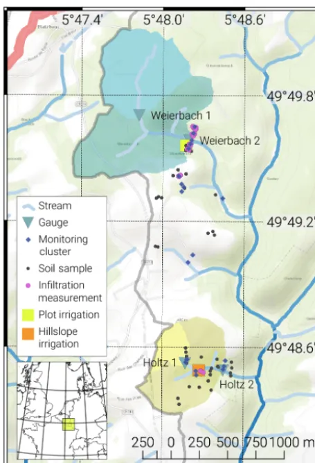
place in stands of spruce,Picea abies). The agriculturally used plateaus at the hilltops are not examined here. Figure 1 presents a map of the area and the location of the respective measurements and experiments.
2.2 Pedo-physical exploration
The soil physical exploration addressed our research ques-tion Q1 using an intenques-tionally large set of hydrological and geophysical methods to survey the subsurface. The sampling is guided by a network of hydro-meteorological monitoring stations measuring all relevant fluxes and states in the atmo-spheric boundary layer and the subsurface (research project “Catchments As Organized Systems”, Zehe et al., 2014). 2.2.1 Sampling design
or-Figure 1.Map of the study sites in the upper Attert basin, Luxem-bourg.
der to address plot-scale (few meters) and hillslope-scale (a few hundred meters) heterogeneity, the design consisted of clustered sets of point measurements along two catenas plus one set at the site of the hillslope irrigation experiment pre-sented in Sect. 2.4. A detailed map is included as Fig. B1 in the Appendix.
The distance between the clustered sets was 80–200 m. In each, three nested sets with a lag distance of 10–20 m along and perpendicular to the contour line were defined. In such a nested set at least one measurement of infiltration capac-ity and two profiles (laterally spaced 1 m) of saturated hy-draulic conductivity in different depth levels were conducted. To complete the scale triplet (Bloschl and Sivapalan, 1995), the respective support is given in the description of each tech-nique.
In addition to the point measurements, a series of percus-sion drilled profiles (drill head diameter of 4 cm) as 1-D pro-files were drawn and 250 mL ring samples were taken within the top 0.6 m for laboratory analyses.
2.2.2 Exploration techniques
Infiltration capacity was measured at 40 points with a Hood Tension-Infiltrometer (IL-2700, UGT GmbH). It employs a tension chamber (12.4 cm radius) as infiltration water supply. Inside the chamber, a defined low negative pressure head is established, which allows a precise measurement of infiltra-tion capacity at different tensions. Three to five tension levels between the 0 and 5.5 cm water column were applied at each spot.
In addition to infiltration capacity at the surface, we used a Compact Constant Head Permeameter (CHP, Ksat Inc.) for determination of saturated hydraulic conductivity in 32 borehole profiles with 3–7 depth levels of about 20 cm incre-ments, with the lowest level at a depth where further hand-drilling was inhibited by stones. The permeameter estab-lishes a constant water level (10.5 cm in our cases) above the bottom of a borehole (here 5 cm in diameter). The out-flow is measured to calculate saturated hydraulic conductiv-ity (Amoozegar, 1989).
The 63 undisturbed soil ring samples were analyzed for bulk density, porosity (assumed to be equal to saturated soil water content), soil water retention properties (Hyprop, UMS GmbH and WP4C Decagon Devices Inc.), saturated hydraulic conductivity (Ksat, UMS GmbH), and soil texture (ISO 11277, wet sieving and pipette method sedimentation). 2.3 Imaging and quantification of rapid flow in
plot-scale irrigation experiments
In order to explore the network of flow-relevant structures and patterns of rapid subsurface flow, we conducted three plot-scale irrigation experiments. This relates to our second research question Q2. The general setup is very similar to the one described by Allroggen et al. (2015b), van Schaik (2009), Öhrström et al. (2004) and Kasteel et al. (2002). Marked on the map in Fig. 1, the three plots are located on a forested mid slope near gauge Weierbach 2 (see also Fig. B1).
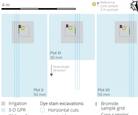
2.3.1 Experimental design and multi-method approach Three plots of 1 m2size were irrigated each for 1 h with an intensity of 50, 30, and 50 mm h−1on 30 October, 1 Novem-ber, and 2 November 2013, respectively. The relatively high rates were chosen to activate the potential flow paths, thereby establishing connectivity. A layout of the experiment is pre-sented in Fig. 2.
The irrigation was accomplished by spray irrigation (full-cone nozzle Spraying Systems Co.) using a wind-protection tent. Brilliant Blue dye tracer (4 g L−1) and bromide salt (5 g L−1 potassium bromide) were used for qualitative and quantitative reference, respectively.
[image:4.612.54.282.65.399.2]4 m
Irrigation 3-D GPR
TDR profile Vertical faces
Horizontal cuts
Bromide sample grid Core samples Plot X
50 mm Plot XI 30 mm
Plot XII 50 mm direction
Reference core sample 3 m upslope
Downslope
[image:5.612.55.280.70.257.2]Dye stain excavations:
Figure 2.Plan view layout of the plot-scale irrigation experiments.
Three irrigation plots (1 m2, gray squares) are monitored by
3-D time-lapse GPR (blue rectangles) and T3-DR (soil moisture tube probe, red box). The plots are sampled for tracer recovery by per-cussion drilled core samples (yellow dot) and in a grid on the last of three vertical faces (dashed blue line). Moreover, dye stains are ex-cavated at horizontal cuts in the center of the irrigation area (dashed blue square). A pre-irrigation reference for porewater stable isotope composition is sampled as a fourth core 3 m upslope.
through continuous TDR measurements in an access tube (Pico IPH, IMKO GmbH) down to 1.5 m depth and with a diameter of 4.2 cm. This technique is chosen to minimize the impact of sensor installation (percussion drilling and instal-lation of the tubes from the surface) and to avoid interfer-ence with the GPR (sensor probe was removed during GPR measurements). The sensor measured an integral of about 1 L (depth increment of 18 cm, mean signal penetration of 5.5 cm). It was manually lowered in the tube to the respective depth for each reading. Each measurement took about 10 s. Hence the whole procedure added up to 4–10 min per profile record. The procedure was continuously repeated until 1.5 h after irrigation onset in line with the findings of Germann and al Hagrey (2008) and Germann and Karlen (2016). They pro-pose that film flow in soil structures disperses into the matrix after 1.5 times the duration of a constant plot irrigation.
Two hours after the end of each irrigation, a percussion drilled soil core was taken (drill head diameter of 8 cm) and sampled in 5 cm depth increments down to 1 m. The plot was excavated 24 h after irrigation for vertical and horizontal re-covery of Brilliant Blue stains. This was done by successive digging of three vertical faces into the plot (aligned with the slope line, 0.1 m distance starting from the lateral edge) and five to seven horizontal cuts in different depth levels down to the first deposit layer (0.5×0.5 m2in the center of the plot). On the third vertical face in the center of the plot core sam-ples of 66 mL soil were taken in a 5 cm grid with 5 columns
and 14–21 rows. In order to minimize time lags in the 70– 105 individual samples, a quick-sampler (see Appendix A) was developed, allowing for precise and nearly undisturbed sampling.
2.3.2 Bromide recovery and stable isotope analysis All samples were analyzed for bromide (Br−). This was done by oven drying the samples and consecutively suspend-ing them in 150 mL de-ionized water (72 h in an overhead shaker at nine rotations per minute). The samples were then left 4 days for sedimentation to exfiltrate the excess through (a) filtration paper (5–13 µm) and (b) 0.45 µm PP micro-filter. The extracts were analyzed in an ion chromatograph (Metrohm 790 Personal IC) with an anion separation column (Metrosep A Supp 4 – 250/4.0) for Br−concentration.
A recovery coefficient (RC) is calculated as proportion of recovered mass of Br−in the soil samples scaled to the total
irrigated area times the depth of the lowest sample. Through this we neglect lateral flow from the irrigation spot and fur-ther percolation in the calculation. We also assume the sam-ples to be representative for the whole affected soil volume.
Prior to the bromide analysis, the percussion drilled soil core samples were also analyzed for their stable isotopic composition (δ18O and δ2H) of the porewater. See Ap-pendix D for details and results, which are given in compari-son to the bromide recovery.
2.3.3 Calculation of apparent vertical flow velocity The quantitative measurements allow one to infer apparent vertical flow velocity along the profiles. For bromide we em-ploy a cumulative curve method (Leibundgut et al., 2011). The distribution of the advective velocityvadvectis set to the
depth distribution of the tracer concentration at the time of fixationtfix. For the profile we assume apparent velocities:
v=z/tfix. (1)
Relating to our third research question Q3, they are projected to the recovered distribution of tracer concentration:
8(vadvect,z)=ctracer,z/ zmax
X
z=0
ctracer, (2)
wherezis depth and8is the cumulative distribution func-tion. Obviously, the estimated travel velocity distribution de-pends strongly on the selection of tfix somewhere between
2.3.4 Analysis of soil moisture responses
The individual TDR soil moisture measurements (θ) were projected to a regular grid of 0.1 m depth increments and 10 min time increments for visualization of changes com-pared to the initial records. As an alternative and indepen-dent estimate of vertical response velocities (research ques-tion Q3), we calculated the distribuques-tion of first exceedance of soil moisture by≥2 % vol in each depth levelz:
vresponse=z/t1θ≥0.02. (3)
For this the un-interpolated measurements were used. 2.3.5 3-D time-lapse GPR
GPR is known as geophysical imaging technique with high spatial resolution (Huisman et al., 2003; Binley et al., 2015). Applied at the shallow subsurface it has been proven as potential means to locate and characterize soil layers and subsurface structures (Holden, 2004; Gormally et al., 2011; Steelman et al., 2012; Klenk et al., 2015). GPR is also ca-pable to monitor subsurface fluid migration in time-lapse ap-proaches (Birken and Versteeg, 2000; Trinks et al., 2001). Our experiments were monitored by 3-D time-lapse GPR measurements as described by Allroggen et al. (2015b). We employed a PulseEKKO Pro GPR system (Sensors and Soft-ware Inc.) equipped with 500 MHz shielded antennas with constant offset of 0.18 m. Sampling interval was set to 0.1 ns, recording a total trace length of 100 ns in 8 internal stacks. Since precise positioning and accurate repeatability are key requirements, we used a kinematic survey approach rely-ing on an automatic-trackrely-ing total station (Leica Geosystems AG, providing sub-centimeter coordinates) in combination with a portable measuring platform (Allroggen et al., 2015b). Using this setup, we acquired one 3-D GPR data cube be-fore irrigation, one directly after the end of irrigation, and a last one about 20 h after irrigation for each plot. One sur-vey took about 45 min. Allroggen and Tronicke (2016) have shown that a pixel-to-pixel comparison of the radar ampli-tudes (A) is not suitable for analyzing time-lapse GPR data in the presence of limited repeatability and noisy data. They propose a structural similarity attribute inspired by (Wang et al., 2004) calculated in a moving window. It normalizes the cross-correlation cx,y of the residuals (A−µA) of two
different acquisition times (x, y) by the product of their stan-dard deviations (σA). They further introduceda as 10% of
the maximum amplitude to avoid numerical instabilities with near-zeroσ values:
Sstruct(x, y)=
cx,y+a
σAxσAy+a
. (4)
In our study we calculate the structural similarity at-tributeSstructof the pre-irrigation reference and the two
post-irrigation records using a local Gaussian window of 2.5 ns along the vertical axis and 0.1 m along the horizontal axis.
The attribute ranges between 1 and−1, with 1 being highly similar and−1 referring to most dissimilar. Points of low similarity indicate deviations that arise from changes in di-electric permittivity which likely reflect changes in local soil water content.
As an additional estimate of vertical response velocities, the same approach as for the soil moisture responses (Sect. 2.3.4) was employed with a threshold of the similarity at-tribute of zero between pre- and post-irrigation records. 2.4 Lateral subsurface flow paths in the hillslope In order to examine the characteristics of flow-relevant struc-tures and the periglacial deposit layers at the hillslope scale, we conducted an experiment on 21 June 2013 at a close-by hillslope. The experiment was specifically designed to ex-plore the response in lateral preferential flow paths and to replicate the plot-scale experiments without tracer applica-tion. The site had to be chosen for facilitation reasons (per-missions, accessibility, collaboration within the CAOS re-search project). With reference to its hydrological responses (companion paper Angermann et al., 2017, this issue), vege-tation, slope, soils and hydraulic properties, we consider the hillslopes to be very similar.
2.4.1 3-D GPR survey of the hillslope
As an additional reference to the soil core profiles, a 3-D GPR survey of the hillslope was conducted prior to the nat-ural event and the irrigation. The GPR data processing relies on a standard processing scheme including bandpass filter-ing, zero time correction, envelope-based automatic scalfilter-ing, gridding to a regular 0.03 m by 0.1 m grid, inline fk-filtering and a 3-D topographic migration approach as presented by Allroggen et al. (2015a), using an appropriate constant ve-locity of 0.07 m ns−1.
For structural analysis, the processed data are imported into the OpenDtect software (dGB Earth Sciences). Under heterogenous soil conditions the derived data cube is domi-nated by complex reflection patterns which prohibit a classi-cal structural analysis based on picking reflectors (as done in a study with a similar cope but different setting by Gormally et al., 2011). Therefore, we support our interpretation of the 3-D GPR data and picking of potential flow-relevant horizons by a dip-corrected semblance attribute. The attribute calcu-lates the spatial coherency and highlights areas of coherent reflections (Marfurt et al., 1998). Low semblance indicates more complex reflection patterns caused by high internal het-erogeneity, possibly influencing the subsurface flow regime. 2.4.2 Experimental design
monitoring area, all shrubs were carefully removed from the experimental site to accomplish GPR measurements and al-low for undisturbed and homogeneous irrigation. The topo-graphic gradient is about 14◦.
Irrigation area | Downhill area 6 5 4 2 1
TDR 17
1 2 3
GPR 4
(a)
Hillslope
cross section
Core area
1
11 12
13 14
17
5 6
7 8
9
2 4
10
TDR 18
1 2 3 GPR 4
5 m
Core area
3
(b)
Plan
view
Sprinkler Irrigated area Rain shield
[image:7.612.58.279.128.444.2]TDR profile GPR transect
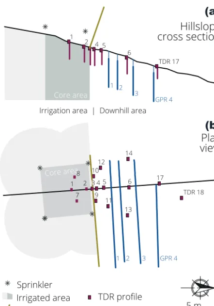
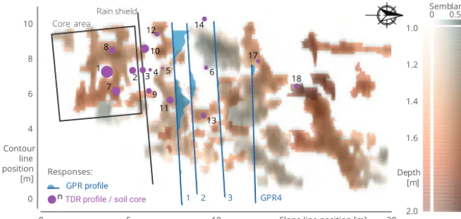
Figure 3.Layout of the hillslope-scale irrigation experiment as
ver-tical view(a)and plan view(b). The hillslope is divided into an
irrigation area and a downhill area by a rain shield. Sixteen access tubes for TDR measurements of soil moisture profiles are arranged in three diverting transects. Parallel to the contour lines, four tran-sects of 2-D time-lapse GPR are recorded.
The experimental layout is given in Fig. 3. Irrigation inten-sity, the duration of the experiment and the spacing of the ob-servation profiles have been decided based on a priori mod-eling scenarios as described in Appendix C. The experiment was preceded by two strong storm events of 43 mm in total on 20 June. The events ended 20 h before irrigation onset. The irrigation of 141 mm in 4.5 h was fed from stream water and was realized by four circular sprinklers (Wobbler, Senninger Irrigation Inc.) arranged to overlap at a 5 m by 5 m core area with relatively homogeneous intensity. While boundary ef-fects were mitigated by an irrigated buffer zone of about 4 m at the uphill and lateral borders of the core area, the down-hill boundary was defined by a rain shield. This established a sharp transition to the non-irrigated area below. Water col-lected by the rain shield was routed off the experimental site. Irrigation was monitored by a flow meter to measure the
ab-solute water input, one tipping bucket to monitor the tempo-ral variability, and 42 mini rain collectors evenly distributed across the core area to check spatial heterogeneity of the in-tensity.
Moreover, a surface runoff collector was installed across 2 m of the lower boundary of the core area. It was built from a plastic sheet installed approximately 1 cm below the interface between litter layer and Ah horizon of the soil profile. At the downhill end of the sheet, the water was captured by a buried and covered gutter. An in-ground tube was attached to the deepest point of the gutter to conduct the water to a tipping bucket downhill of the investigated area. The tube had been filled with water prior to the experiment to ensure an immediate reaction to the occurrence of surface runoff.
We monitored soil moisture dynamics in a setup of 16 ac-cess tubes with 3 manual TDR probes like in the plot-scale experiments (Imko GmbH, two with 12 cm integration depth and one with 18 cm). Measurements required manual posi-tioning of the sensor probes for each reading. We continu-ously recorded the states in all tubes in 10 cm depth incre-ments, realizing revisiting intervals of 5–20 min. The tubes were installed to reach to a depth of about 1.7 m. The layout consisted of three diverging transects with four TDR profiles in the lower half of the core area, the highest density of files just downhill from the rain shield, and the furthest pro-file about 9 m downhill.
Four 2-D time-lapse GPR transects were treated as
GPR-inferred, non-invasive trenchesparallel to the contour lines
located 2, 3, 5, and 7 m downhill from the rain shield. Here, the GPR acquisition unit was equipped with shielded 250 MHz antennas. The data were recorded using a constant offset of 0.38 m, a sampling interval of 0.2 ns and a time win-dow of 250 ns. Wooden guides and the automatic tracking total station guaranteed accurate and repeatable positioning. 2.4.3 Analysis of TDR data
In order to synchronize the almost 5000 individual TDR soil moisture records to a regular grid in time and depth, interpo-lation and resampling were required. To do so, we generated an intermediate grid of high data density onto which linearly interpolated versions of the time series of each profile were projected. We then resampled from this intermediate grid to derive a synchronized version of the records at 0.1 m depth and 15 min time increments. With this the spatial aggregation remains below the integration length of the TDR probes.
The temporal resampling and the therefore necessary lin-ear interpolation is close to the acquisition timing of one profile (4–10 min each). Since the correlation length of dis-tributed soil moisture observations is rather short and be-cause we explicitly aim to analyze the responses of prefer-ential flow structures, the issue of interpolation needs special attention and will be discussed in Sect. 4.2.1.
onset to identify activated flow paths. Lateral interpolation between different TDR profiles over distances of about 1 m and above is unfeasible. Soil moisture as extensive state vari-able is discontinuous at interfaces. The found subsurface set-ting does not exhibit any isotropic continuum required for such interpolations.
As in the plot irrigation experiments, vertical response ve-locities are calculated for the TDR profiles in the core area. The calculation of lateral response velocities is given in the companion study (Angermann et al., 2017, this issue). 2.4.4 GPR transects and structural similarity attribute
interpretation
The 2-D time-lapse GPR data are derived from nine repeated recordings along the four vertical GPR transects. Each record is processed after a standard processing scheme of band-pass filtering, zero time correction, exponential amplitude preserving scaling, inline fk-filtering, topographic migration with constant velocity (0.07 m ns−1), and consecutive grid-ding to a 2-D transect with regular trace-spacing of 0.02 m.
Most time-lapse GPR data analyses are based on calcu-lating trace-to-trace differences (Birken and Versteeg, 2000; Trinks et al., 2001) or picking and comparison of selected reflection events in the individual time-lapse transects (All-roggen et al., 2015b; Haarder et al., 2011; Truss et al., 2007). Like in the 3-D time-lapse GPR applications, the radargrams in the young, highly heterogeneous soils do not exhibit ex-plicit reflectors as suitable references. In addition, the limited repeatability of the measurements and the desired identifica-tion of lateral flow structures require an alternative approach. Like for the plot-scale experiments, we use the time-lapse structural similarity attribute (Allroggen and Tronicke, 2016, and Sect. 2.3.5). It is calculated using a local Gaussian win-dow of 2 ns along the vertical axis and 0.06 m along the hor-izontal axis.
Due to the presence of remaining event water from the pre-ceding storm event (Angermann et al., 2017, this issue), all measurements are referenced to the last acquisition time ap-proximately 23 h after irrigation start and about 19 h after ir-rigation. The resulting structural similarity attribute images are used as a qualitative indicator of relative deviations from the reference state.
2.4.5 Discriminating the natural storm event and the irrigation experiment
The experiment was preceded by two strong storm events of 43 mm in total on 20 June 2013. In reference to the gauge re-action the experiment was conducted shortly before the sec-ond peak of the runoff reaction to the preceding storm events (see Fig. 5 in Angermann et al., 2017, for details). Accord-ingly, the structural similarity attributes, which compare the distributed states at the respective acquisition time to the last record, identify responses to both drivers, the natural storm
event and the irrigation experiment. To discriminate the sig-nals we analyze the dynamics of each pixel in the GPR tran-sects over time. The first two structural similarity attribute transects 7.5 h before and directly at irrigation start are at-tributed to the natural event and show an increasing struc-tural similarity (towards accordance with the reference state). Once the attribute value of a pixel decreases again (increas-ing deviation from the reference state) it is attributed to the irrigation. For stability reasons, a threshold of 0.15 was in-troduced for the attribute to be exceeded to detect changes. This is discussed in Appendix F.
3 Results
3.1 Soil physical exploration
3.1.1 Point samples show high heterogeneity
The in situ point measurements of infiltration capacity and saturated hydraulic conductivity showed high variability without clear relationships with simple morphological de-scriptors like depth, hillslope position or topographic flow gradient (details given in Fig. B1). Infiltration capacity ranged from 5×10⁻⁵ to 5×10⁻³m s−1. The values for saturated hydraulic conductivity ranged from 1×10⁻⁸ to 1×10⁻³m s−1and even exceeded the measuring range of the constant head permeameter. Only at the site of the hillslope-scale experiment was a pattern of elevated conductivity at about 0.6 m depth found. The strong heterogeneity and large spread of values was also depicted in the analyses of undis-turbed soil samples (Fig. 4).
On average the area is dominated by silty soils (see also Juilleret et al., 2011). This was corroborated by texture analy-ses and the mean retention characteristics. However, the mea-surements of saturated hydraulic conductivity are on average 2 orders of magnitude larger than what might be expected for these soils given their texture (Schaap et al., 2001). Also, porosity clearly exceeds the expected values, while bulk den-sity is smaller than expected (compare Fig. 4, middle row of the panels). All measurements exhibited a large spread of val-ues which does not correlate well with simple morphological variables like depth or hillslope position (Fig. 4, bottom row). The high hydraulic conductivity and large porosity is maybe explained by aggregation of fine silty material in conjunction with a network of rapidly draining inter-aggregate pores. 3.1.2 Soil core profile snapshots
Be-0.5 1.0 1.5 2.0 2.5 0.4 0.6 0.8 −7 −6 −5 −4 −3 −2
Ksat [ms-1] Porosity
[m³m-³]
Bulk density
[gcm-³]
Literature reference
Cl
SiCl SaCl
ClLo SiClLo
SaClLo
Lo
SiLo SaLo
Si LoSa
Sa
80 60 40 0
0 20
40 60
Clay [%]
Silt [%]
Sand [%] Texture
20
40
60
0 1 2 3 4 pF 6
0.0 0.1 0.3 0.4 0.5
0.2 theta [m³m-³]
Average
retention
Clay loam
0.0 Sample depth [m] 0.3 0.4 0.5 0.6 0.7 0.8 0.9
0 1 2 3 4 pF 6
0 Distance to stream [m] 75 100 125 150 175 200 225 250 10 10 10 10 10 10
10-6 10-4 10-2
0.0
Depth [m] 0.2
0.3
0.4
0.5
Ksat [ms-1]
10-6 10-4 10-2
0.0 0.1 0.2 0.3 0.5
Gravel content [gg-1]
Silty clay
loam
0.0 0.2 0.5 0.9 Depth [m]
Soil water retention (drying)
Rosetta reference
(a)
(b)
[image:9.612.82.505.68.492.2](d)
(c)
Figure 4.Results of laboratory analyses of 63 undisturbed 250 mL ring samples.(a)Soil texture analyzed with wet sieving and sedimentation (pipette method). Saturated hydraulic conductivity (Ksat) measured with the Ksat apparatus and plotted against sample depth and gravel
content. Black box plots of the respective depth increment.(b)Histograms and kernel density estimate of measured bulk density, porosity
and Ksat. Reference as the mean silty loam value from the literature (Hillel, 1980; Rawls et al., 1982; Carsel and Parrish, 1988). Rosetta
(Schaap et al., 2001) reference based on mean values of samples (15.7, 47.9, 36.4 % sand, silt, clay and BD 1.1 g cm−3).(c)Soil water
retention relation measured with the Hyprop and the WP4C apparatus with the average retention estimate (respective mean of each 0.05
pF-bin and fitted van Genuchten model) and literature references (Carsel and Parrish, 1988) scaled to measured averageθsandθr.
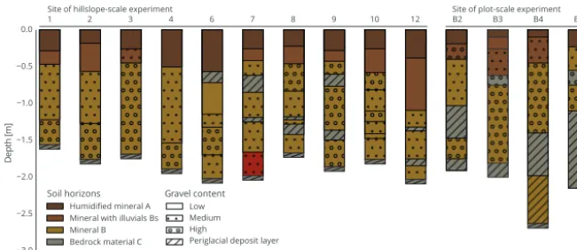
low the depth of 0.5 m, scattered layers of weathered rock with usually horizontal orientation were found in some soil cores. Percussion drilling was often inhibited at a depth be-tween 1.5 and 2.0 m (lower end of the bars in Fig. 5) due to even higher stone content with a more and more vertical ori-entation of the weathered rocks. In core 7, concretions of iron and manganese oxides were found at depths between 1.6 and 1.9 m below ground, indicating hydromorphic conditions.
Based on these standard techniques the overall setting of a heterogeneous silty soil deviating from expected low
1 2 3 4 6 7 8 9 10 12 B3 B4 B7
−3.0 −2.5 −2.0 −1.5 −1.0 −0.5 0.0
De
pt
h
[m
]
Humidified mineral A
Mineral with illuvials Bs
Mineral B
Bedrock material C
Gleying, redox iron Cg
Low
Medium
High
Periglacialdeposit layer
Soil horizons Gravel content
[image:10.612.132.458.67.208.2]Site of hillslope-scale experiment Site of plot-scale experiment B2
Figure 5.Soil core profiles from the upper Colpach River basin. See Figs. 3 and B1 for positions. Bar depth is the maximum drilling depth of the cores restricted by large stones or bedrock.
3.2 Plot-scale flow path activation and vertical velocities
3.2.1 Irregular patterns of dye stains
In the plot-scale tracer experiments the Brilliant Blue dye stains identified patchy infiltration patterns partially bypass-ing large sections of the soil without clear traces of the ac-tual flow path (Fig. 6). For all experiments stained patches were found down to the periglacial deposit layer at 0.6–0.8 m depth. During the excavation apparently isolated dye traces were recovered even several meters downhill from the irri-gation spot (4 m downslope, 1 m deep). The stains did not reveal a network of large macropores but an irregular mesh of connected inter-aggregate voids. This is in line with the observed hydraulic capacity (Fig. 4).
3.2.2 Bromide breakthrough to the periglacial deposit layer
The connectedness and large transport capacity of this net-work of inter-aggregate pores is corroborated by the distribu-tions of bromide tracer recovery (Fig. 7, top row). All plots suggested a relatively strong response at a depth of approxi-mately 0.6 m. This depth correlates with the upper boundary of the first layer of periglacial deposits found in core pro-file B3 (Fig. 5) and in the excavated soil propro-files. This re-sponse is contrasted by low bromide concentration at a shal-lower depth. Even plot XI, where only 30 mm were applied, showed the same pattern with a clear breakthrough to the periglacial deposit layer.
At plot XII we found a stronger interaction with the soil matrix, which led to more dye staining and a higher bromide recovery. Overall, tracer recovery was incomplete (0.45, 0.38, and 0.83 for plots X to XII, respectively) and even declined when including the core samples (0.24, 0.3, 0.63) once more, pointing to strongly irregular soil water re-distribution.
Figure 6. Recovered dye patterns in plot irrigation experiments.
(a)Excavated vertical faces, (b) horizontal cuts in 0.5 m depth.
Dashed lines indicate level of periglacial deposit layer.
3.2.3 Quick soil moisture response in greater depth The observed soil moisture changes (Fig. 7, bottom row) cor-roborated the results from the tracer data. Especially at plot X and XII we found a relatively quick and strong response at 0.7 and 0.5 m depth, respectively. This even preceded soil moisture changes in shallower layers in plot X. Hence the records highlighted an important characteristic of the identi-fied flow-relevant structures, although the signal had a much lower spatial resolution than the tracer results. In contrast to the recovered tracers, we did not observe significant changes in soil moisture in plot XI. This can be explained by its posi-tion offset from the main flow field (Fig. D2 in Appendix D). 3.2.4 3-D view on soil water redistribution
[image:10.612.313.543.263.436.2]0 0.1 0.2 [m] m(Br-)[mg] ∆θ [vol%] referred to pre-irrigation state 0 10 20 30
m(Br-)[mg] m(Br-) [mg] m(Br-)[mg] 60 −1.0 −0.4 −0.2 0.0 D ep th [m ]
Plot XII, RC=0.83/0.63
0 0.1 0.2 [m] 0 10 20 30 60
−1.0 −0.4 −0.2 0.0 D ep th [m ]
Plot XI, RC=0.38/0.3
0 10 20 30 40
−1.0 −0.4 −0.2 0.0 D ep th [m ]
(a) Bromide recovery [mg]
Plot X, RC=0.45/0.24
0 6 24 30 36 42 48 54 60
0.0 0.4 0.8 1.2 Time [h] Profile Core
(scaled)
Profile Core
(scaled)
Profile Core
(scaled)
0.0 0.4 0.8 1.2 Time [h] 0.0 0.4 0.8 1.2 Time [h]
−1.0 −0.4 −0.2 0.0 D ep th [m ] −1.0 −0.4 −0.2 0.0 D ep th [m ] −1.0 −0.4 −0.2 0.0 D ep th [m ] 20 15 10 5 0 -5 TDR measurements
0 0.1 0.2 [m] (b) Soil moisture change ∆θ
[image:11.612.130.469.71.240.2]Plot X | | Plot XI Irrigation period Plot XII
Figure 7. Results from plot-scale irrigation experiments with 50, 30, and 50 mm spray irrigation for 1 h.(a)Recovered bromide mass
profiles and grids (5×5 cm). Blue line as mean and shaded area between min/max for each depth of the sampling grid. Orange line is the
mass recovered in drilled profile samples (scaled to the same volume reference). Recovery coefficient (RC) calculated for the profile samples
(first value) and the profile and core samples (second value).(b)Observed soil moisture change referenced to the first measurement shortly
before onset of the irrigation. Individual measurement times marked with triangles.
in soil moisture in a spatial context. At all plots the response patterns of low structural similarity pointed out quick ver-tical flow to a depth of 80 ns or about 1.4 m within 1.5 h after irrigation start (Fig. 8, and Figs. D2 and D3 in Ap-pendix D). Also here, strongest deviations were recorded in the mid horizon between 40 and 60 ns two way travel time (TWT) corresponding to approximately 0.7 to 1 m depth. The top horizon between 20 and 40 ns (0.35–0.7 m) had compa-rably high similarity. Measurements above that depth were technically not possible. Patches of low structural similarity until 20.5 h after irrigation start suggested further lateral re-distribution in the later course of the experiment at plot X. At plot XI with 30 mm irrigation further vertical transport with a slight lateral component was recorded. Plot XII had a very high similarity between the first and third acquisitions. This is a sign of stronger macropore–matrix interaction and dispersive redistribution.
The contrasting attribute distributions over time and com-paring plots X and XII not only revealed diverse patterns. It also highlighted the qualitative nature of the analytical method of the GPR data. Although visual interpretation of the radargrams (top rows in Figs. 8, D2 and D3) is very dif-ficult, they show how the structural similarity attribute high-lighted areas where radar patterns changed. Due to the com-plex reflection energy patterns it is not suitable to trace in-dividual reflectors. This prevents a quantitative interpretation as shown by Allroggen et al. (2015b).
For the identification of structures, the results did not ex-hibit specific macropores like the dye stains, but areas of re-sponse to the irrigation. Nevertheless, the patchy characteris-tic of the found response patterns was very similar to that of Brilliant Blue.
3.2.5 Derivation of vertical flow velocities
Based on all applied techniques, hydraulic conductivity and apparent vertical flow velocities were calculated (kernel den-sity estimates plotted in Fig. 9). The many point-scale mea-surements (left panel based on 63 ring samples, 40 infiltrom-eter points, 102 individual permeaminfiltrom-eter measurements) re-sulted in disagreeing distributions stretching across a large spectrum of flow velocities. The reason for this spread stems from the fact that the measurements consist of matrix flow and flow in structures. The response-related methods of the irrigation experiments were in much better accordance be-cause they all relate to the same processes. They revealed an apparent vertical velocity of 1×10−3.5m s−1(Fig. 9b, based on bromide recovery with an estimated time of fixation (tfix)
after 1.5 h, first excess of TDR recorded soil moisture≥2 % vol, and GPR structural similarity attributes below zero be-tween pre-irrigation and the first post-irrigation records).
All results ranged several orders of magnitude above the literature reference of 2.5×10⁻⁷m s−1 (mean of reported values for silt and silty loam – Hillel, 1980; Rawls et al., 1982; Carsel and Parrish, 1988) and the Rosetta value of 6.2×10⁻⁶m s−1 (Schaap et al., 2001). The role of inter-aggregate pores facilitating this quick redistribution even through comparably small voids without noticeable dye staining was corroborated.
0.5 0.9 1.3 1.7 2.1 2.5 2.9 3.3
Slope line distance [m] 20
40 60 80
TW
T
[n
s]
0.5 0.9 1.3 1.7 2.1 2.5 2.9 3.3
Slope line distance [m] 20
40 60 80
0.5 0.9 1.3 1.7 2.1 2.5 2.9 3.3
Slope line distance [m] 20
40 60
80 −
+
0.0 0.4 0.8 1.2 1.6 2.0 2.4 2.8 3.2 3.6 0.0
0.4 0.8 1.2 1.6 2.0
C
ontour line distance
[m]
0.0 0.4 0.8 1.2 1.6 2.0 2.4 2.8 3.2 3.6 0.0
0.4 0.8 1.2 1.6 2.0
0.0 0.4 0.8 1.2 1.6 2.0 2.4 2.8 3.2 3.6 0.0
0.4 0.8 1.2 1.6 2.0 0.0 0.4 0.8 1.2 1.6 2.0 2.4 2.8 3.2 3.6
0.0 0.4 0.8 1.2 1.6 2.0
C
ontour line distance
[m]
0.0 0.4 0.8 1.2 1.6 2.0 2.4 2.8 3.2 3.6 0.0
0.4 0.8 1.2 1.6 2.0
0.0 0.4 0.8 1.2 1.6 2.0 2.4 2.8 3.2 3.6 0.0
0.4 0.8 1.2 1.6 2.0
−1.0 −0.8 −0.6 −0.4 −00.0.2 0.2 0.4 0.6 0.8 1.0 GPR amplitude
Structural similarity attribute Top
Mid
Low
Slope line distance [m] Slope line distance [m] Slope line distance [m]
Center line radargrams 0:00 h 1:00 h 20:00 h
1:00 h Low 1:00 h
20:00 h Mid 20:00 h Low 20:00 h
Top
Structural similarity attribute of 3-D time-lapse GPR
Top 1:00 h Mid
Center line radargram position
[image:12.612.129.468.69.285.2]Irrigation plot
Figure 8.Time-lapse 3-D GPR of irrigation experiment at plot X. Center line radargrams at the marked transect (gray dashed line in lower panels) for the three acquisition times (before 0:00 h, directly after irrigation 1:00 h, 20:00 h after irrigation) are given in the top row. Two way travel time (TWT) is given as original depth reference. The structural similarity attribute of the 3-D data cube is given in three different depth layers (top 20–40 ns, mid 40–60 ns, low 60–80 ns) in the lower panels. The irrigation plot is marked by a black dashed box/line. Slope line distance is increasing downslope.
−7 −6 −5 −4 −3 −2 −1
(a)ksat log10 [m s-1] Lab Hood CHP CHP CHP top 2nd low
−5.5 −5.0 −4.5 −4.0 −3.5 −3.0 −2.5 (b) Apparent velocity log10 [m s-1]
Bromide (t = 1.5 h) TDR response GPR response fix
Rosetta mean
t 6 h 3 h 1.5 h 1 h
fix
Figure 9.Saturated hydraulic conductivity and apparent vertical flow velocity kernel density estimates.(a)Point-scale measurement results
(Lab: Ksat apparatus; Hood: Hood Tension-Infiltrometer; CHP: Constant Head Permeameter in different depth levels);(b)results from
plot-scale irrigation experiments. Vertical gray lines are box plots of velocity distribution based on differenttfixestimates for bromide. Rosetta
(Schaap et al., 2001) reference based on mean values of ring samples (15.7, 47.9, 36.4 % sand, silt, clay and BD 1.1 g cm−3).
(Fig. 10). This is in accordance with the soil core profile depth (Fig. 5). Especially profile 7 suggested an imperme-able layer just below that depth. Although a potential struc-ture can be identified, it remains unclear to which degree this area of high spatial inhomogeneity in terms of radar reflec-tion characteristics is flow-relevant, unless a reacreflec-tion to an event is observed.
3.3.2 Hillslope responses
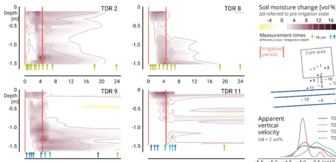
The results of the hillslope-scale irrigation experiment can be distinguished into the core area observations with TDR profiles only and observations at the downhill monitoring area, including TDR profiles as well as 2-D GPR transects. The change in soil moisture at the core area (TDR 2 and 8
[image:12.612.128.467.368.459.2]con-0 5 10 Slope line position [m] 20 0
Contour line position [m]
4 6 8
10 Core area
Rainshield
1
10
11 12
13 14
17
18
2 3 4 5 6
7 8
9
1 2 3 GPR4
0 0.5 1
Semblance
Depth [m] 1.0
1.2
1.4
1.6
2.0 TDR profile / soil core
GPR profile n
[image:13.612.131.467.68.228.2]Responses:
Figure 10.Potential subsurface structures from 3-D GPR survey and setup of hillslope experiment. Structure identification guided by the
dip corrected semblance attribute. Depth estimated based on mean measured effective radar velocity in soil of 0.07 m ns−1. Summary of
the hillslope experiment given by locations of TDR profile tubes (purple, also location of respective soil cores in Fig. 5) and GPR transects (blue). Dot size of TDR scaled to maximum of observed change in soil moisture. Along GPR transects lateral marginals of the structural similarity attribute as proxy for recorded advection. Note that the picked potential subsurface structures are located in different depth (white to black) and that variations in spatial contrast can be seen in the semblance attribute (white to orange). Where more than one horizon has been identified the top one is plotted.
nection. Overall changes in soil moisture as a maximum at each TDR profile did not corroborate the potential subsur-face structures identified in the 3-D GPR survey (compare identified potential structures with dot sizes in Fig. 10). The full set of profiles is reported in the companion study (Anger-mann et al., 2017, this issue).
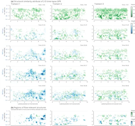
The four successive GPR transects across the downhill monitoring area provided spatially distributed images of hillslope-scale flow patterns and boundary fluxes. The struc-tural similarity attribute of storm event water (green) and ir-rigation water (blue) revealed distinct, heterogeneously dis-tributed patterns (Fig. 12) pointing to discrete connected flow paths instead of an irregular network of inter-aggregate pores. The measurements suggested that lateral flow takes place in a very diverse network with very low similarity be-tween the transects. Moreover, the responses to the irrigation decayed with distance to the core area.
The patches which reacted to the storm event are mostly different ones than the structures used to drain the irrigation water. Apparently the irrigation experiment initiated flow in more shallow structures (compare transect 1 irrigation reac-tion with transect 3 storm water in Fig. 12). Areas of high temporal dynamics of the similarity attribute were identified as regions of such flow-relevant structures (Fig. 12, bottom row). Note that the last recorded difference 18 to 23 h af-ter irrigation start (not shown) exhibited high similarity in all profiles. The mean of the attribute was between 0.93 and 0.96 and standard deviation between 0.076 and 0.048 for GPR transects 1 and 3, respectively. Apparently, the system had reached a steady state without much further change in soil moisture (see Appendix F for more details).
The patchy structures at the transects highlighted the ir-regularly distributed nature of lateral preferential flow paths which was similarly observed in the plot experiments. Al-though some areas exert a higher density of reacting flow paths than others, no continuous patterns could be specified throughout the hillslope. We also saw a decay of the signal strength and areal share with distance from the core area. As the patterns from transect 1 did not simply propagate fur-ther downslope, the flow paths must be tortuous and leaky. Hence inferring the configuration of the connection between the four transects in the downhill direction is not feasible. A comparison of the suggested structures of the 3-D GPR survey to the overall response to irrigation recorded at the GPR transects did not correlate well (compare identified po-tential structures with the reaction summary at GPR transects in Fig. 10).
4 Discussion
4.1 Identification of flow-relevant structures across scales
Figure 11.Development of soil moisture in TDR profiles during and after the hillslope irrigation experiment. Exemplary transect with changes referenced to pre-irrigation conditions and attributed to irrigation water. Time is given in hours after irrigation start. Individual measurements and probe reference marked with triangles. More data and explanation in Angermann et al. (2017), this issue. Right bottom:
apparent vertical flow velocity as first excess of1θ≥2 % vol at core area profiles.
because of its scale below the support of the measurements. Vice versa, methods at the next scale do not provide informa-tion about porosity and bulk density.
Irrigation experiments at the plot scale visualized that a network of these inter-aggregate voids connects the surface to the periglacial deposit layer and is responsible for highly diverse soil water redistribution. These structures are differ-ent from what we usually expect (cracks, worm burrows, roots channels) at this scale. This could be depicted from dye tracer stains (Fig. 6), which still have the highest spa-tial resolution on the cost of a lack of temporal insight. It requires strong assumptions about macropore–matrix inter-action, time of fixation and dye supply, retention and recov-erability. Despite all uncertainty about what process caused staining, the technique allows to identify the structures ac-tivated by irrigation and to infer much about their setting where dye has been retained. Although dye stains are closely related to actual flow and thus function, they only reveal the potential pathways and thus form as the actual processes and timing remain unknown. When irrigation intensity and irrigation amount ranges near the hydraulic capacity of the macropore network while still avoiding ponding or macrop-ore clogging, the entire network of flow-relevant structures is marked. 3-D time-lapse GPR has proven to be capable to detect similar response patterns. However, the spatial and temporal resolution of the method is still insufficient to de-tect the flow-relevant inter-aggregate voids marked by dye stains. Some of the structures have not even been traced with dye, nor could GPR identify them. Nevertheless, the overall characteristics of the structures as patchy responses are depicted well and in a non-invasive, spatially continu-ous manner. Thus most of the point-sampling related issues (Sects. 3.1.1 and 4.4) are resolved. Regarding research ques-tion Q2, the visualizaques-tion of flow structures based on
re-sponses to irrigation succeeded at the plot scale. They are in good coherence with the quantitative findings from salt trac-ers, stable isotopes and soil moisture dynamics. Interestingly, the found vertical response velocity distributions correspond well to the saturated hydraulic conductivity measurements in soil samples, although their distribution is much more tight.
At the hillslope scale (Q3), applications of 3-D time-lapse GPR are technically impossible due to the long acquisition times. Consequently we altered the setup to four trench-like 2-D time-lapse GPR profiles to facilitate the required high temporal resolution. The responses suggest structures similar to but less diverse than the found inter-aggregate voids at the plot scale. They are spatially persistent and leaky and appar-ently feed from diverse sources. As such the irrigation exper-iment caused a similar response in different structures than the previous storm event. Moreover, the relatively high input rates have proven adequately chosen to identify lateral sub-surface flow paths. At this scale the capability of point-based methods for structure identification is even more limited as the dense network of soil moisture profile observations did not allow the derivation of a conclusive picture.
4.2 Event response patterns reveal flow-relevant structures
0 2 4 6 8 10 0 −1 −2 −3 −4
Time: -7:33 Transect 1 0 29 57 86 114 TWT [ns] E st. depth [m]
0 2 4 6 8 10
0
−1
−2
−3
−4
Time: 01:25
0 29 57 86 114 TWT [ns] E st. depth [m]
0 2 4 6 8 10
0
−1
−2
−3
−4
Time: 03:18
0 29 57 86 114 TWT [ns] E st. depth [m]
0 2 4 6 8 10
0
−1
−2
−3
−4
Time: 05:14
0 29 57 86 114 TWT [ns] E st. depth [m]
0 2 4 6 8 10
0
−1
−2
−3
−4
Time: 06:43
0 29 57 86 114 TWT [ns] E st. depth [m]
0 2 4 6 8 10
Lateral position on transect [m] 0 −1 −2 −3 −4 0 29 57 86 114 TWT [ns] E st. depth [m]
0 2 4 6 8 10
0
−1
−2
−3
−4
Time: -7:35 Transect 2
0 2 4 6 8 10
0
−1
−2
−3
−4
Time: 01:27
0 2 4 6 8 10
0
−1
−2
−3
−4
Time: 03:20
0 2 4 6 8 10
0
−1
−2
−3
−4
Time: 05:17
0 2 4 6 8 10
0
−1
−2
−3
−4
Time: 06:44
0 2 4 6 8 10
Lateral position on transect [m] 0
−1
−2
−3
−4
0 2 4 6 8 10
0
−1
−2
−3
−4
Time: -7:37 Transect 3
0 2 4 6 8 10
0
−1
−2
−3
−4
Time: 01:29
0 2 4 6 8 10
0
−1
−2
−3
−4
Time: 03:23
0 2 4 6 8 10
0
−1
−2
−3
−4
Time: 05:20
0 2 4 6 8 10
0
−1
−2
−3
−4
Time: 06:46
0 2 4 6 8 10
Lateral position on transect [m] 0
−1
−2
−3
−4
Lateral position on transect [m] Lateral position on transect [m] Lateral position on transect [m]
(b) Regions of flow-relevant structures
Standard deviation of structural similarity attribute over time
(a) Structural similarity attribute of 2-D time-lapse GPR
[image:15.612.82.518.69.477.2]−0.5 0.0 0.5 1.0 Irrigation −0.5 0.0 0.5 1.0 Storm 0.1 0.5 0.1 0.5 Irrigation Storm
Figure 12.Structural similarity attribute in time-lapse 2-D GPR transects. Blue: irrigation event water; green: storm event water. Columns:
time series in one transect; rows: different transects at the same time.(b)Identified regions of rapid subsurface flow based on the standard
deviation of all structural similarity attributes at one transect over time. Note: the structural similarity attribute calculates similarity between the radargram at the respective time to the last record 23 h past irrigation. A threshold of 0.15 is applied to identify significant changes. It is a qualitative measure based on the assumption that the last record is in steady state and that all differences are induced by soil water redistribution.
4.2.1 Soil moisture responses
In our case TDR measurements through access tubes were employed as low-impact means to monitor soil water dy-namics in order to detect areas of quick and strong response. Structures in general and the inter-aggregate voids in our case cover only a very small fraction of the measured volume. We may underestimate detected flow paths when they do not al-ter the total volumetric soil waal-ter content much (bypassing). This can explain the observed patterns of low response in the topsoil and changes in regions where the fast flow is deceler-ated at some kind of bottleneck. Referring to the theoretical
integration volume of 1 L, it would require a macropore of about 1 cm diameter within the support of the sensor to be filled to just reach a threshold of 2 % vol. Adding this 20 mL of water diffusively would result in the same measurement. This shows that soil moisture measurements exhibit a con-ceptual bias towards the diffusive fraction of the soil water.
Com-paring the identified regions of flow structures (Fig. 12) with the support of a TDR sensor quickly reveals that even a large number of point observations remains highly uncertain if the overall spatial context is unknown. This is especially the case at the hillslope scale. At the plot scale, the issue is less pro-nounced, as we have shown with the good correspondence between tracers, GPR and soil moisture reaction at plot X (Figs. 7 and 8). However, at plot XI with less intense irri-gation, the soil moisture profile did not react despite the evi-dence of quick vertical redistribution in all the other methods. Apparently, the TDR records were simply not close enough to the relatively few activated flow paths (Fig. D2).
4.2.2 Time-lapse GPR patterns
The potential horizons identified by the static 3-D GPR sur-vey do not coincide with the observed responses (Fig. 10). This is another example for the requirement of a shift be-tween active and non-active state to identify flow-relevant structures. The structural similarity attributes derived from time-lapse GPR reveal the patterns of soil water redistribu-tion. The continuous 2-D and 3-D data allow to relate tempo-ral changes in space as images of the subsurface as proposed by Gerke et al. (2010); Beven and Germann (2013) and oth-ers.
The comparison of radargrams in time needs further at-tention: In other time-lapse GPR applications for soil water dynamics in structured domains (Truss et al., 2007; Haarder et al., 2011; Allroggen et al., 2015b; Klenk et al., 2015) anal-ysis is guided by reference to a reflector and its apparent displacement can be used to calculate changes in soil mois-ture. Alternatively, a wetting front could generate a reflector (Léger et al., 2014). In our case none of these existed.
On the one hand, we minimized methodological prob-lems concerning the noise arising from the imperfect posi-tioning of repeated GPR measurements by using a measur-ing platform at the plot scale, transect guides at the hills-lope scale, and an automatic-tracking total station (Allroggen et al., 2015b). On the other hand, we base our analysis on the structural similarity attribute instead of pixel-to-pixel com-parison or picked reflectors. The disadvantage is that this al-lows only for a qualitative measure. The advantage is that the spatial organization of areas with changing reflection and transmission properties (which are attributed to changes in soil moisture) can be revealed even in heterogeneous soils. The 3-D applications at the plot scale avoid strong assump-tions about the continuity of preferential flow paths when inferring 3-D networks from 2-D measurements (Gormally et al., 2011; Guo et al., 2014). Especially in the soils under study, the found response patterns (Fig. 8) and the excavated stained soil profiles (Fig. 6) show highly tortuous flow paths. Thus we refrain from interpolations between the multi-2-D transects at the hillslope scale.
Although the 3-D time-lapse attribute data of the plot ir-rigation experiments are of low spatial resolution (blur due
to similarity attribute method and long duration of one ac-quisition) and limited temporal resolution (few acquisition times), they are suitable to identify regions of flow-relevant structures and their characteristics. In the multi-2-D transects resolution was enhanced (short duration of one acquisition and many repeated measurements) which depicted the struc-tures much better. Hence, time-lapse GPR can especially be improved by enhancing the acquisition time and frequency.
The observation of changes during activation of flow-relevant structures generated the required contrast to overall heterogeneity. For large structures, this ledto precise identi-fication and localization. Smaller flow paths cannot be fully resolved. Nevertheless, the continuous 2-D and 3-D images of the subsurface response patterns provide means to non-invasively study the form–function relationship in situ and to overcome some of the restrictions of retrospective and de-structive tracer methods. However, quantitative interpretation of time-lapse GPR data remains challenging.
4.3 Methodological assessment
In contrary to our first expectation, the value of pedo-physical analyses of soil core samples has been relatively high even for characteristics of flow facilitated by the re-vealed paths at larger scales. Structure identification is not only obscured in heterogeneity as one would expect, but properties deviating from the standard situation (fine texture, low bulk density and high porosity) gave rise to the identifi-cation of the inter-aggregate flow paths. However, the spatial organization of structures below and above the support of the samples cannot be revealed. This is also the reason for the relatively low information which could be drawn from the in situ infiltration measurements: The observed flow rates are largely affected by the capacity of the connected flow paths draining the measurement point. This adds to the critical as-sumption of homogeneity (Langhans et al., 2011).
Besides the high information gain through the state shift of flow-relevant structures in irrigation experiments, the em-ployed methods at the plot scale have very specific advan-tages and disadvanadvan-tages: Especially the laborious and costly analysis of salt tracers and stable isotopes is contrasted by relatively little additional information. Moreover, the lack of a temporal information about when the solute or water molecule was retained in a certain depth is seen problematic. Soil moisture profile dynamics and time-lapse GPR do not suffer this drawback. Both can be employed with very low or even no impact on the subsurface from the surface. While GPR requires to be operated in higher temporal resolution (see Sect. 4.5), soil moisture profiles lack the desired spatial discretization. Dye staining delivers the highest spatial reso-lution to reveal subsurface structures on the cost of blindness about the temporal dynamics. Furthermore, a tomographic excavation of the stains has proven very difficult.