Empirical Mode Decomposition on the sphere: application to the spatial scales of surface temperature variations

www.hydrol-earth-syst-sci.net/12/933/2008/ © Author(s) 2008. This work is distributed under the Creative Commons Attribution 3.0 License.

Earth System

Sciences

Empirical Mode Decomposition on the sphere: application to the

spatial scales of surface temperature variations

N. Fauchereau1, G. G. S. Pegram2, and S. Sinclair2

1_{Department of Oceanography, University of Cape-Town, Cape Town, South Africa} 2_{Civil Engineering, University of KwaZulu-Natal, Durban, South Africa}

Received: 2 January 2008 – Published in Hydrol. Earth Syst. Sci. Discuss.: 15 February 2008 Revised: 15 May 2008 – Accepted: 19 May 2008 – Published: 20 June 2008

Abstract. Empirical Mode Decomposition (EMD) is applied here in two dimensions over the sphere to demonstrate its potential as a data-adaptive method of separating the differ-ent scales of spatial variability in a geophysical (climatologi-cal/meteorological) field. After a brief description of the ba-sics of the EMD in 1 then 2 dimensions, the principles of its application on the sphere are explained, in particular via the use of a zonal equal area partitioning. EMD is first applied to an artificial dataset, demonstrating its capability in extract-ing the different (known) scales embedded in the field. The decomposition is then applied to a global mean surface tem-perature dataset, and we show qualitatively that it extracts successively larger scales of temperature variations related, for example, to topographic and large-scale, solar radiation forcing. We propose that EMD can be used as a global data-adaptive filter, which will be useful in analysing geophysical phenomena that arise as the result of forcings at multiple spa-tial scales.

1 Introduction

Variability in the climate system occurs at a large range of space and time scales. One challenge of climate data analysis is to separate these scales and their interactions. This issue is important for the understanding and the prediction of the variability of the climate of the Earth. If one can identify the intrinsic scales of variations, extract the corresponding signal and analyse the relationships with other signals, at the same or at a different level, one can then get an idea of the relationships, in terms of physical or statistical dependency, of variability at different scales.

Correspondence to: G. Pegram ([email protected])

For the last 50 years or so a great deal of effort has been put into the development, refinement and application of statisti-cal methods that help to achieve the goal of separating signal from noise and identifying the preferred scales of variations in both time and space.

In one dimension, variations can be separated using Fourier series, wavelets, Singular Spectrum Analysis, etc. The power spectrum of a one dimensional time-series can be decomposed into its preferred frequency components, hence the preferred time-scales of variations. However, though widely used, these methods rely on quite strong assumptions: most especially stationarity and/or the choice of predefined basis functions.

In space, the problem of scale separation is much more difficult. If time is a natural, sensible direction along which perform the analysis in one dimension, in two dimensional space there is no obvious and natural preferred direction. So on a global scale, it would be arbitrary, although convenient if one is using Fourier or Wavelet methods, to perform scale separation following e.g. only latitudes and longitudes. Fur-thermore, although there are definite periodicities in the rota-tion of the Earth, weather and climate are not truly periodic, so the use of a lat-long co-ordinate system is pertinent only when one searches a-priori for given structures (e.g. wave-like patterns at high latitudes). However, this analysis pre-supposes that we have an a-priori knowledge of the form of the embedded scales.

variations in both in time and space. Singular Spectrum Analysis (Elsner and Tsonis, 1996), has also been used in this context for a number of years.

Recently a new method, namely Empirical Mode Decom-position (called EMD hereafter) was introduced by Huang et al. (1998) for the analysis of 1-D signals in the context of time-series analysis. The basic idea of EMD is to allow for an adaptive and unsupervised representation of the basic components of linear and non-linear signals and is designed to accommodate non-stationarity in the series.

This method has recently been extended to two dimensions (Linderheld, 2002; Nunes et al., 2003). The 2-D decompo-sition has also been used in the context of the analysis of radar rainfall fields at high resolution by Sinclair and Pegram (2005) where a full justification for the method is available, an outline will be offered later in this paper.

One of the difficulties associated with 1-D EMD is the treatment of the ends of the bounding functions, requiring some (non-objective) decisions to be made in order to pro-ceed (Chiew et al., 2005; Peel et al., 2005; Pegram et al., 2008). In the application of 2-D EMD in radar fields, the edges of the wet areas are well defined, so the ending prob-lem is solved, since the envelopes of the extrema at any stage of the decomposition process are set implicitly to zero.

The beauty of decomposing a field on the sphere is that there are no edge or end effects. What is more, on the sphere, it is particularly advantageous to dispense with a formal co-ordinate system and to compute the distances between points of interest (extrema in the decomposition process), as one would do in Kriging a field of randomly arranged points in 2-D. It is precisely this thinking that allows us to treat each observation with the same weight, in contrast with methods applied to the lat-long grid which cannot sensibly ascribe the same weight to values at high as well as low latitudes.

The goal of this paper is to demonstrate how 2-D EMD can be applied on the sphere to separate different spatial scales embedded in a field. 2-D EMD will be applied in this context as a data-adaptive spatial filter to successively remove the smaller scale variations and retain only the larger ones.

The paper is organized as follows: Sect. 2 presents the zonal equal area partitioning of the sphere, used to ade-quately represent the data on the sphere on equal areas for the requirements of the EMD analysis. Section 3 presents an out-line of the basic principles and algorithm of the EMD in one dimension, while the fourth section presents the principles of its extension to the 2-D case on a sphere. The algorithm is then applied on a simple artificial dataset to demonstrate its viability in Sect. 5. In Sect. 6, a first application on the Surface Temperature field obtained from a reanalysis is then presented and we show how EMD on the sphere can be used to filter out the local scales of variations and retain only the larger ones. Conclusions, future developments and potential applications are discussed in Sect. 7.

2 The zonal equal area partitioning of the sphere

The first step is to find an appropriate projection to repre-sent/map the data on the sphere for the purpose of 2-D EMD analysis.

Global-scale climatological data, whether it comes from observations, numerical model outputs, reanalyses, etc. are usually provided on a regular grid, for which the number of longitude points per latitude is always the same, so that for a 2.5◦resolution, one obtains a 72×144 matrix. This presents a set of problems: i) the data points are not representative of equal areas; at the equator the mean area for a standard 2.5◦ resolution grid is 12 345 square kilometers, while near the poles, at 87.5 degrees, it is 538 km2, i.e. reduced by a factor of 23 ii) the data at the pole are surrogate, stretched along the longitudes to match the regular grid.

The properties of the physical space that are required for EMD to work without supervision are two: i) continuous (no edges) ii) the points should be relatively equidistant, i.e. rep-resentative of a roughly equal area. Thus, in order to apply the EMD on the sphere, we need to first resample/interpolate the original data onto a physical partitioning of the sphere that matches these requirements.

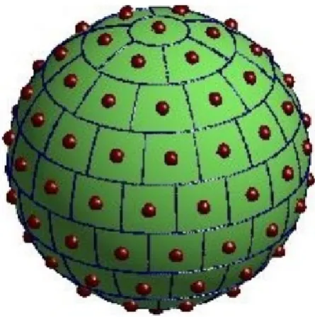
Recently, a method for equal area partitioning of the sphere that respects these requirements has been presented (Leopardi, 2006). A Recursive Zonal Equal Area partition is a partition ofSdim(the unit sphere in the dim+1 Euclidean spaceRdim+1)into a finite number of regions of equal area. The area of each region is defined using the Lebesgue mea-sure inherited from Rdim+1. Each region is defined as the product of intervals in spherical polar coordinates. The cen-tre point of a region (element) is defined via the cencen-tre of each interval, with the exception of the polar caps, where the centre of the region is simply the centre of the spherical cap (hence the geographical pole). One of the advantages of this partitioning (in contrast to triangulation which was consid-ered but rejected) is that each edge of the spherical trapezium lies on a latitude or longitude, making interpolation from a lat-long grid relatively easy. Figure 1 provides an example of a partition ofS2into 100 elements of equal area.

For a partition of the sphere into 6500 elements, the num-ber of latitude bands is 73, and the maximum numnum-ber of lon-gitude separations (symmetrical each side of the equator at

3 The basic principles of the EMD in one dimension

The basic idea embodied in the EMD analysis, as introduced by Huang et al. (1998), is to allow for an adaptive and un-supervised representation of the intrinsic components of lin-ear and non-linlin-ear signals based purely on the properties ob-served in the data, without appealing to the concept of sta-tionarity. As Huang et al. (1998) point out in their abstract: “This decomposition method is adaptive and therefore highly efficient. Since the decomposition is based on the local char-acteristic time scale of the data, it is applicable to nonlinear and non-stationary processes.”

Few sequences of observations of natural phenomena are long enough to test the hypothesis of stationarity and fre-quently, the phenomena are patently non-stationary. The EMD algorithm copes with stationarity (or the lack of it) by ignoring the concept, embracing non-stationarity as a prac-tical reality. For a fuller discussion of the genesis of these ideas, see the Introduction of Huang et al. (1998), who also heuristically demonstrate the implicit orthogonality of the se-quences of Intrinsic Mode Functions (IMFs) defined by the EMD algorithm.

In the application of the 1-D EMD algorithm, the possibly nonlinear signal, which may exhibit varying amplitude and local frequency modulation, is linearly decomposed into a finite number of mutually quasi-orthogonal, zero mean, fre-quency and amplitude modulated signals, as well as a resid-ual function which (i) exhibits a single extremum, (ii) is a monotonic trend or (iii) is simply a constant. Although EMD is a relatively new data analysis technique, its power and sim-plicity have encouraged its application in many fields. It is beyond the scope of this paper to give a complete review of the applications, however a few examples are cited here to give the reader a feeling for the broad scope of applications. Chiew et al. (2005) examine the one-dimensional EMD of several annual streamflow time series to search for signifi-cant trends in the data, using bootstrapping to test the statis-tical significance of identified trends. The technique has been used extensively in the analysis of ocean wave data (Huang et al., 1999; Hwang et al., 2003) as well as in the analysis of polar ice cover (Gloersen and Huang, 2003). EMD has also been applied in the analysis of seismological data by Zhang et al. (2003) and has even been used to diagnose heart rate fluctuations (Balocchi et al., 2004). The algorithm for 1-D EMD is readily available in the cited literature, so is not re-peated here; the 2-D extension is based on the 1-D algorithm and is elaborated in Sect. 4.

4 The extension of EMD to 2 dimensions on the sphere

The 2-D EMD process is conceptually the same as in one dimension, except that the curve fitting of envelopes to the maxima and minima now becomes a surface fitting exercise and the identification of the local extrema is performed in

Fig. 1. A Zonal Equal Area partition of the sphere using 100 points.

space to take into account for the connectivity of the points. There is one difference in performing EMD on the sphere as against on a surface with edges, like a flat map: there are no edges requiring special treatment as the surface is fully con-tinuous. The introduction to the 2-D EMD method applied on a 2-D plane, and references to earlier supporting work, are fully described by Sinclair and Pegram (2005), so only the essentials are repeated here.

2-D EMD provides a truly two-dimensional analysis of the intrinsic oscillatory modes inherent in the data. Two-dimensional Fourier and Wavelet analyses are really appli-cations of their one-dimensional counterparts in a number of principal directions. Fourier analysis concentrates on orthog-onal “East-West” and “North-South” directions (e.g. Press et al., 1992). Wavelet analysis can, in general, consider any di-rection of the wavelet relative to the data, however a typical 2-D Wavelet analysis examines only horizontal, vertical and diagonal orthonormal wavelet basis functions (Daubechies, 1992, pp. 313; Kumar and Foufoula-Georgiou, 1993). In contrast, EMD produces a fully two dimensional decomposi-tion of the data, based purely on spatial reladecomposi-tionships between the extrema, independent of the orientation of the coordinate system in which the data are viewed. There is also a small change in terminology: in place of Implicit Mode Functions (IMFs) in 1-D EMD, we choose to use Implicit Mode Sur-faces (IMSs) in 2-D EMD.

4.1 Description of the algorithm

The algorithm follows intuitively from the one-dimensional case. We consider a two-dimensional data-setz(θ, α), where

latitude and longitude to describe it’s location on a sphere. The decomposition may then be obtained as follows:

1. Set the (zeroth) residualr0(θ, α)=z(θ, α)and seti=1

2. Locate the extrema ofri−1(θ, α)in the 2-D space

in-cluding maximal and minimal plateaux. On a rectangu-lar grid, this is done by finding those points in the cen-ter of a 3×3 square of pixels which are larger/smaller than any of the eight surrounding points. On the sphere partitioned using the Zonal Equal Area algorithm, it is sufficient to identify the extrema relative to the centres of the six closest surrounding elements, because of the staggering of the successive rings of elements.

3. Generate the bounding envelopes to the extrema, maxi−1(θ, α)and mini−1(θ, α), using appropriate

sur-face fitting techniques. We suggest Kriging with an exponential semivariogram whose correlation length is set equal to double the average spacing between the elements at each stage of the decomposition. This choice yields a relatively smooth surface without iso-lated peaks.

4. Compute the mean surface function of the local aver-age value of the upper and lower envelopes fitted to the extrema,mi−1(θ, α)=[maxi−1(θ,α)

+mini−1(θ,α)]

2

5. Determine the first estimate of an IMS by sub-tracting the mean surface from the current residual IMSi(θ, α)=ri−1(θ, α)−mi−1(θ, α).

6. Iterate over steps 2-5 until IMSi is close to zero

every-where (settingri−1=IMSi before each iteration).

7. The Residual accepted after iteration is now calculated asri(θ, α)=ri−1(θ, α)−IMSi(θ, α).

8. If the Residualri(θ, α)is a constant or has a single

ex-tremum, then stop; else incrementiand return to step 2.

4.2 Surface fitting for extremal envelope generation The generation of maximal and minimal envelopes is of key importance to a successful 2-D EMD implementation and is the most computationally intensive task. The problem is a familiar one of collocating a smooth surface to randomly scattered data points in two-dimensions. There are several options available to achieve this. Ultimately the fitting pro-cedure reduces to computing the unknown value of the sur-face at a point si=(xi, yi), by some linear (or nonlinear)

weighting of the known data. In general, a basis function determines the influence of each known data point based on its spatial position relative to the unknown pointsi. Nunes

et al. (2003) and Delechelle et al. (2005) use radial basis functions while Linderhed uses bi-cubic splines (Linderhed, 2002) and later chooses the more suitable option of Thin

Plate Splines (Linderhed, 2004). We tried radial basis func-tions (technically, conical Multiquadrics), which are iden-tical to Kriging (Cressie, 1991) with a purely linear semi-variogram model, but they produced spurious local extrema which only showed up in the IMSs. We decided it would be more appropriate to select an exponential variogram to model the envelopes of the maxima and minima. We choose a corre-lation length equal to the average distance between extrema at any stage of the decomposition, invoking Occam’s razor in the spirit of Huang’s original derivation of EMD. The bound-ing surfaces are then generated usbound-ing Ordinary Krigbound-ing, en-suring that the surfaces are constrained to tend towards the mean surface of the extrema at distance.

In essence, the 2-D EMD algorithm on the sphere pro-vides a complete quasi-orthogonal decomposition of the data, hence allows for a summation of the data over a range of scales, thus providing, by analogy to the digital filter of one-dimensional vectors, a data-adaptive spatial filter.

5 Application to an artificial example

In order to test the 2-D algorithm on the sphere in controlled conditions, an artificial global dataset was first created by summing two different fields with contrasting patterns and different spatial scales.

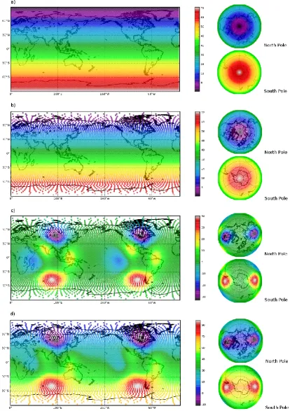
The first field (Fig. 2a and b) consists of a simple merid-ional gradient from the North to the South pole. It constitutes the largest spatial scale of the artificial field.

The second field (Fig. 2c) has been constructed as a mix of scaled and translated Gaussian functions. It is assumed here to represent relatively small scale variations of the scalar field embedded in the larger spatial scale presented by the above gradient.

The artificial field analysed simply consists of the sum of the two interpolated fields and is presented in Fig. 2d.

The 2-D EMD algorithm was then applied to this artificial dataset to see if it is able to retrieve the two different fields that constitute it.

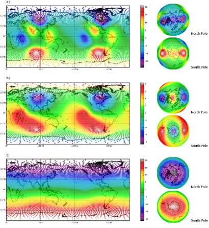
Fig. 3. (a) The 1st IMS of the artificial field, it’s variance is equal to 129.0. (b) The 2nd IMS of the artificial field, it’s variance is equal to

10. (c) The 3rd IMS of the artificial field, it’s variance is equal to 125.3.

Table 1. Variance explained by each of the IMSs obtained from

the decomposition of the ERA surface temperature field shown in Fig. 4. The variances are expressed as a percentage of the variance in the original field. The 5th residual is constant with no variance.

IMS1 IMS2 IMS3 IMS4 IMS5

percent. variance 30.8 42.5 25.5 0.9 0.3

6 Application to surface air temperature

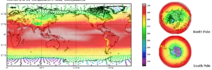
The surface air temperature (at 2 m) used here has been extracted from the ERA 15 reanalysis project (http://www. ecmwf.int). It is available on a 2.5×2.5◦regular grid from at a monthly time-step from January 1979 to December 1993. We make use here of the long-term annual mean computed from the monthly values. The field, shown interpolated on the zonal equal area partition of the sphere, is presented in Fig. 4.

Fig. 4. ERA 15 surface temperature long-term mean (1979–1993): interpolated onto a zonal equal area partitioning of the sphere using 6500

points.

at different scales, from small-scale temperature contrasts to the global scale related to the temperature gradient from the tropics to the poles.

The 2-D algorithm is then applied to the temperature field presented in Fig. 4 in the same way as it was applied to the artificial dataset presented in Sect. 5.

Here 5 IMSs are extracted before obtaining a residual con-stant field (of value 286.3). The variance explained by each IMS is presented in Table 1.

The 2 last IMSs have a very low variance and can safely be pooled with the 5th residual to form the 3rd residual.

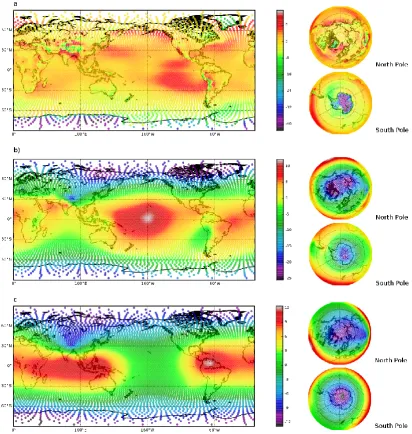
The first IMS (Fig. 5a) represents the high frequency sig-nal embedded in the temperature field. The most striking fea-tures are the local high spatial variances associated with high mountainous areas such as the Andes and the Himalayas. The Antarctic and Greenland Ice-Caps and the strong tem-perature gradients associated with the relatively warmer sur-rounding ocean masses are also responsible for large local variability. As such and as expected, the 1st IMS accounts mainly for the small scale variability in the surface tempera-ture field associated with local forcings.

The second IMS (Fig. 5b) represents clearly larger scale variations and has the highest variance. The variance is re-lated to a large extent to the temperature gradient from the tropics to the poles, that is forced by the distribution of so-lar radiation. A very prominent feature also extracted on this IMS is the presence of large areas of high temperature values found in the Pacific Ocean, which we attribute to the warm pool.

The third IMS (Fig. 5c), is related again to the large-scale gradient from the tropics to the poles, minus the prominent warm pool region that has been extracted in the 2nd IMS.

The results presented above confirm that the 3 first IMSs qualitatively represent three different and hierarchical scales of the spatial organization of the global mean temperature: local to regional scale variations linked to the topography and the presence of ice-caps, the prominent warm pool region in the pacific, and the large-scale gradient from the tropics to the poles related to mean solar forcing.

As the sum of the all the IMSs plus the final residual is exactly equal to the original field (see Sect. 3), one then can use 2-D EMD as a filter to remove from a field the high fre-quency variations, as a data-adaptative spatial filter. The field in Fig. 6 has been obtained by summing IMSs 2 to 5 with the 5th residual and is therefore equal to the first residual. The effect is to filter out the smaller scale topographically forced variations extracted in the 1st IMS. The resulting field shows the contribution of large scale forcings to global mean sur-face temperature.

7 Conclusions

Empirical Mode Decomposition has been applied to the anal-ysis of a two-dimensional field on the sphere, taking advan-tage of the data-adaptive nature of the method and the ab-sence of edge or end effects on the sphere. In addition, the interpolation of data from a regular grid to a zonal equal area partition of the sphere allows each observation to be treated with the same weight.

Fig. 5. (a) The 1st IMS produced when performing EMD on the ERA 15 surface temperature field. (b) The 2nd IMS produced when

performing EMD on the ERA 15 surface temperature field. (c) The 3rd IMS produced when performing EMD on the ERA 15 surface temperature field.

The potential applications of EMD on the sphere for cli-mate data are numerous: in the context of statistical analysis of space-time climate variability, the algorithm can be used prior to traditional techniques (such as PCA/EOF) to uncover the intrinsic spatial scales contained in a field and filter out the unwanted scales of variations. EMD could also be used, in the context of numerical simulations on Atmospheric Gen-eral Circulation Models, to create forcing fields having pre-defined scales of spatial variation. We propose EMD on the sphere as an appropriate a adaptive and largely data-driven exploratory analysis tool for global geophysical data. Acknowledgements. The authors wish to acknowledge support from the French-South African SAFeWater program administered by the South African Water Research Commission, which provided support to bring us together to collaborate – A new Entente Cordiale.

Edited by: M. Sivapalan

References

Balocchi, R., Menicucci, D., Santarcangelo, E., Sebastiani, L., Gemignani, A., Gellarducci, B., and Varanini, M.: Deriving the respiratory sinus arrhythmia from the heartbeat time series us-ing Empirical Mode Decomposition, Chaos Soliton. Fract., 20, 171–177, 2004.

Chiew, F. H. S., Peel, M. C., Amirthanathan, G. E., and Pegram, G. G. S.: Identification of oscillations in historical global stream-flow data using Empirical Mode Decomposition, in: Regional Hydrological Impacts of Climatic Change Hydroclimatic Vari-ability, Proceedings of Symposium S6 held during the Seventh IAHS Scientific Assembly at Foz do Iguac¸u, Brazil, IAHS Publ., 296, p. 5362, 2005.

Cressie, N.: Statistics for Spatial Data, Wiley, New York, 1991. Daubechies, I.: Ten Lectures on Wavelets, Society for Industrial

and Applied Mathematics, Philadelphia, Pennsylvania, 1992. Delechelle, E., Nunes, J., and Lemoine, J.: Empirical mode

decom-position synthesis of fractional processes in 1D and 2D space, Image Vision Comput., 23, 799–806, 2005.

Elsner, J. and Tsonis, A.: Singular Spectrum Analysis. A New Tool in Time Series Analysis, Plenum Press, New York, 1996. Gloersen, P. and Huang, N. E.: Comparison of Interannual Intrinsic

Modes in Hemispheric Sea Ice Covers and Other Geophysical Parameters, IEEE T. Geosci. Remote, 41, 1062–1074, 2003. Huang, N. E., Shen, Z., Long, S. R., Wu, M. C., Shih, H. H., Zheng,

Q., Yen, N., Tung, C. C., and Liu, H. H.: The Empirical Mode Decomposition and the Hilbert Spectrum for Nonlinear and Non-Stationary Time Series Analysis, Proceedings of the Royal Soci-ety London A, 454(1971), 903–995, 1998.

Huang, N. E., Shen, Z., and Long, S. R.: A new view of Nonlinear water waves: the Hilbert Spectrum, Annu. Rev. Fluid Mech., 31, 417–457, 1999.

Hwang, P. A., Huang, N. E., and Wang, D. W.: A note on analyzing nonlinear and nonstationary ocean wave data, Appl. Ocean Res., 25, 187–193, 1999.

Kumar, P. and Foufoula-Georgiou, E.: A Multicomponent Decom-position of Spatial Rainfall Fields 1. Segregation of Large- and Small-Scale Features Using Wavelet Transforms, Water Resour. Res., 29(8), 2515–2532, 1993.

Leopardi, P.: A partition of the unit sphere into regions of equal area and small diameter, Electron. T. Numer. Ana., 55, 309–327, 2006.

Linderhed, A.: 2D empirical mode decompositions in the spirit of image compression, Proceedings of SPIE, Wavelet and Indepen-dent Component Analysis Applications IXI, 4738, 2002. Linderhed, A.: Adaptive Image Compression with Wavelet

Pack-ets and Empirical Mode Decomposition, Linkoping Studies in Science and Technology, Dissertation No. 909, ISBN 91-85295-81-7, 2004.

Nunes, J. C., Bouaoune, Y., Delechelle, E., Niang, O., and Bunel, Ph.: Image analysis by bidimensional empirical mode decompo-sition, Image Vision Comput., 21, 1019–1026, 2003.

Peel, M. C., Amirthanathan, G. E., Pegram, G. G. S., McMahon, T. A., and Chiew, F. H. S.: Issues with the application of Em-pirical Mode Decomposition Analysis, in: MODSIM 2005 In-ternational Congress on Modelling and Simulation, Modelling and Simulation Society of Australia and New Zealand, edited by: Zerger, A. and Argent, R. M., December 2005, 1681–1687, ISBN 0975840029, 2005.

Pegram, G. G. S., Peel, M. C., and McMahon, T. A.: Empirical mode decomposition using rational splines: an application to rainfall time series, Proc. Royal Soc. A, 464, 1483–1501, 2008. Preisendorfer, R. W.: Principal Component Analysis in

Meteorol-ogy and Oceanography, Elsevier, Oxford, New York, Tokyo, 1988.

Press, W. H., Teukolsky, S. A., Vetterling, W. T., and Flannery, B. P.: Numerical Recipes in C The art of scientific computing, Second Edition, Cambridge University Press, 1992.

Sinclair, S. and Pegram, G. G. S.: Empirical Mode Decomposition in 2D space and time: a tool for spacetime rainfall analysis and nowcasting, Hydrol. Earth Syst. Sci., 9, 127–137, 2005, http://www.hydrol-earth-syst-sci.net/9/127/2005/.