Ben R. Hodges
National Center for Infrastructure Modeling and Management, University of Texas at Austin, Austin, Texas, USA Correspondence:Ben R. Hodges (hodges@utexas.edu)
Received: 2 May 2018 – Discussion started: 25 June 2018
Revised: 4 January 2019 – Accepted: 19 February 2019 – Published: 7 March 2019
Abstract. New integral, finite-volume forms of the Saint-Venant equations for one-dimensional (1-D) open-channel flow are derived. The new equations are in the flux-gradient conservation form and transfer portions of both the hydro-static pressure force and the gravitational force from the source term to the conservative flux term. This approach pre-vents irregular channel topography from creating an inher-ently non-smooth source term for momentum. The deriva-tion introduces an analytical approximaderiva-tion of the free sur-face across a finite-volume element (e.g., linear, parabolic) with a weighting function for quadrature with bottom topog-raphy. This new free-surface/topography approach provides a single term that approximates the integrated piezometric pressure over a control volume that can be split between the source and the conservative flux terms without introducing new variables within the discretization. The resulting conser-vative finite-volume equations are written entirely in terms of flow rates, cross-sectional areas, and water surface eleva-tions –withoutusing the bottom slope (S0). The new Saint-Venant equation form is (1) inherently conservative, as com-pared to non-conservative finite-difference forms, and (2) in-herently well-balanced for irregular topography, as compared to conservative finite-volume forms using the Cunge–Liggett approach that rely on two integrations of topography. It is likely that this new equation form will be more tractable for large-scale simulations of river networks and urban drainage systems with highly variable topography as it ensures the inhomogeneous source term of the momentum conservation equation is Lipschitz smooth as long as the solution variables are smooth.
1 Introduction
The present work evolved out of a frustration with the slow pace of improvement in SVE modeling. Taking a step back-wards, we can ask the following: is there something fun-damental in the common forms of the SVEs that hinders progress? Motivated by an analysis of the equation forms (Sect. 2) and a study of the wealth of past work in the SVEs (Sect. 3), new insights were developed and are presented herein. The fundamental theses of the present work are as follows: (1) conservative formulation of equations should be used for the next generation of river network models, and (2) the appearance of the channel slope (S0) in the SVEs for channels with irregular topography is a principal cause of instabilities and extended computational time. Neither the-sis can be demonstrated herein – this work is merely a first step that provides the theoretical foundations for a conser-vative and inherently well-balanced approach that highlights the minimal level of approximations needed for a SVE form with irregular topography. It remains for future studies to compare models built on these foundations to the existing approaches to determine if the new forms provide significant numerical advantages.
The new conservative form of the SVEs is developed with a goal of addressing challenges associated with mod-eling large-scale 1-D flow network systems. In the process of developing the new form, we will encounter a philosoph-ical question as to whether the primary vertphilosoph-ical variable in a large-scale network solution should be the depth (H) or the water surface elevation (η). Despite this author’s prior work with H primacy (Liu and Hodges, 2014), we shall see that there are advantages to using η, which is identi-cal to the piezometric pressure and hence uniform over a channel cross-sectional area. The quadrature of the subgrid piezometric pressure gradient and subgrid-scale topography can be handled in a single new term that is derived herein. Through this term interesting possibilities for analytically including hyperresolution bathymetric knowledge while re-taining larger computational elements for large-scale model-ing arise. This idea is not fully exploited within the present work, but the framework is developed for others to build upon.
In the remainder of this paper, Sect. 2 provides motiva-tion and context in the differential forms of the SVEs. Sec-tion 3 provides a further overview of SVE modeling in the wide range of conservative and non-conservative forms. A new and complete derivation of the finite-volume form of the conservative 1-D momentum equation with minimal approx-imations is provided in Sect. 4. Approximate forms of the 1-D SVEs are presented in Sect. 5 and the final form of the equations and a discussion of their potential use are provided Sect. 6.
2 Motivation
In reach-scale hydraulic studies, the Saint-Venant equations are almost always solved in a conservative form (e.g., Karel-sky et al., 2000; Lai et al., 2002; Papanicolaou et al., 2004; Sanders, 2001) but usually in a non-conservative form when used in river network hydrology and urban drainage networks (e.g., Liu and Hodges, 2014; Pramanik et al., 2010; Ross-man, 2017; Saleh et al., 2013). Arguably, the reasons are in the difficulty in obtaining a well-balanced model for the con-servative form and the inherent complexities/uncertainties of channel geometry across a large network (see discus-sion in Sect. 3). In general, conservative equation forms are valued as they ensure (with careful discretization) that transport modeling does not numerically create or destroy the transported variable. Indeed, the use of the conservative form for mass conservation is universal in models from hy-draulics to hydrology – it is only for momentum that the non-conservative form remains common.
To set the context for this paper, consider the non-conservative form of the momentum equation that has been used in large river network solutions (Liu and Hodges, 2014)
∂Q ∂dt +
∂ ∂x
βQ
2
A
+gA∂H
∂x =gA (S0−Sf) , (1)
whereQis the flow rate, Ais the channel cross-sectional area,βis the momentum coefficient (associated with nonuni-form velocities integrated overA),gis gravity,His the water depth,S0is the channel slope, andSfis the friction slope. The above equation has immediate physical appeal as each term represents a clearly understood piece of physics; i.e., the rate of change of the flow is affected by the gradient of nonlinear advection, the hydrostatic pressure gradient (driven by water depth), the gravitational force along the slope, and frictional resistance. The equation includes a conservative form of non-linear advection (all the variables inside the gradient), but
gA∂H /∂x is non-conservative (that is,A, which is a func-tion ofH, is outside the gradient). The terms to the right-hand side (RHS) of the equal sign are considered source and sink terms that reflect creation and destruction of momentum. Thus, a conservative form of the above could be formally written as
∂Q ∂dt +
∂ ∂x
βQ
2
A
= −gA∂H
∂x +gA (S0−Sf) , (2)
the smoothness of the source term in Eq. (2) inherently de-pends on the smoothness of the productAS0and compensa-tion by the solucompensa-tion inA∂H /∂x andASf. The key point is that smoothness in the source term is a mathematical neces-sity for the numerical solution of a partial differential equa-tion to be well-posed (Iserles, 1996), but introducequa-tion ofS0 can place smoothness at the mercy of how well the numerical scheme responds to non-smooth forcing.
In general, there is an advantage to having as much of the physics as possible included on the flux-conservative side of the equation, which helps reduce difficulties associated with discretizations of the source terms (e.g., Pu et al., 2012; Vazquez-Cendon, 1999). The standard form of the conser-vative SVEs is arguably the form provided by Cunge et al. (1980), based on a derivation of Liggett (1975):
∂Q ∂dt +
∂ ∂x
βQ
2
A +gI1
=gI2+gA (S0−Sf) , (4) where I1 andI2 are integrated hydrostatic pressure forces across the channel
I1= Z
H
(H−z)Bdz (5)
and along the channel gradients
I2= Z
H
(H−z)∂B
∂xdz, (6)
withH (x)as the water depth,B(x,z)as the channel breadth as a function of elevation and along-stream location, andzas a coordinate direction measured from a common horizon-tal baseline in a direction opposite to gravitational acceler-ation. This form is also used by others with slightly different nomenclature but the same integral terms (e.g., Hernandez-Duenas and Beljadid, 2016; Sanders, 2001; Saavedra et al., 2003). It is convenient herein to call this the Cunge–Liggett form of the SVEs. The key point for both these terms is that they measure the interaction between the free surface and the channel shape; e.g.,I1could also be written as
∂Q ∂dt +
∂ ∂x β
Q
A +gAH =gH
∂A
∂x +gA (S0−Sf) . (8)
Similar to the Cunge–Liggett form, the above uses a math-ematical trick to place one part of the hydrostatic pressure force within the conservative flux gradient, while retaining the remainder as a source term. Thus, we see that the Cunge– Liggett form is not canonical, nor is it a form that necessar-ily better represents the physics. It is merely a form that is (sometimes) convenient for splitting the gradient of the to-tal hydrostatic pressure force into conservative flux and non-conservative source terms.
The above brings up a question: if it is good to shift a por-tion of the hydrostatic pressure from the source to the conser-vative term as in Eqs. (4) and (8), then why not some or all of the gravitational potential associated withgAS0? Under-lying the Cunge–Liggett form and much (but not all) of the literature is the idea thatgAS0is a source term that creates and destroys momentum. But this is also true of the hydro-static pressure gradient and yet we commonly treat a portion within the convective flux. Thus, if Cunge–Liggett Eq. (4) is preferred over the baseline conservative form of Eq. (2) be-cause a portion of the hydrostatic pressure is moved from the source term to the conservative flux term, then an equation that moves some (or all) of the gravitational potential from the source to the flux term should be equally valued. If this argument is accepted, then the preferred differential form for natural channels with the SVEs is none of those presented above, but perhaps an equation of the general form
∂Q ∂dt +
∂ ∂x
βQ
2
A +f1(A, η)
well-balanced methods as discussed in detail in Sect. 3, be-low.
In this paper, complete derivations are presented to show that finite-volume formulations of the SVEs can be generated that are consistent with the general conservative differential form of Eq. (9). The new derivation is intended to bridge the gap between approaches used in high-resolution hydraulic models and those used in large-scale hydrology and urban drainage networks. The derivation provides a form of the SVEs that has mathematical rigor while preserving the sim-plicity of the non-conservative finite-difference discretiza-tions that are common in hydrological and urban drainage literature. Herein, we focus only on the detailed presentation of the new equation form, reserving demonstration in a nu-merical model to future papers.
3 Background
3.1 Origination and use of the SVEs
The original equations of de Saint-Venant (de Saint-Venant, 1871) were written as
dA
dt +
d(AU )
dx =0, (10)
−dη
dx =
1
g
dU
dt + U g
dU
dx + `p
A F
ρg, (11)
whereUis the velocity,`pis the wetted perimeter, andF is the frictional force per unit bottom area along the channel, and other terms are as previously noted. We have taken the liberty of replacing Saint-Venant’s notation ofw,ζ,χ,swith the more modern nomenclature of A, η, `p, x, but other-wise have retained the original form. The momentum equa-tion of de Saint-Venant, Eq. (11), is identical to Eq. (1) if we use Q=AU, Sf=`pF /(gρA), integrate over a cross section with the β coefficient, apply some calculus with the continuity equation, and define η≡H+zb along with
S0= −∂zb/∂x. From a practical perspective, the only thing that a hydrologist really needs to change from the original equation set is to replace the zero on the right-hand side of Eq. (10) with a source term representing the inflow/outflow per unit length from/into the catchment and groundwater. However, from a numerical modeling perspective, Eq. (11) is fundamentally non-conservative and suitable only for dis-cretization in finite-difference forms. Although the full equa-tion set is sometimes called the SVEs, for convenience in ex-position we will use SVE as a shorthand for the momentum equation alone.
The SVEs are ubiquitous in the literature for a wide range of work and have a foundational role in flow-routing schemes in hydrological models and channel network models for ur-ban drainage. However, there is an interesting gap between the equation forms used in large-scale systems and those used in shorter single-reach studies or modeling hydraulic
features. For computational simplicity, large-scale network flow models often use a reduced set of equations, such as the Muskingum, kinematic wave, or the local inertia form (e.g., Wang et al., 2006; David et al., 2011, 2013; Getirana et al., 2017). Herein, we will follow the arguments of Hodges (2013) that we should be using the full SVEs; i.e., reduced-physics models should be seen as a stopgap measure as we wrestle with obtaining satisfactory SVE solution methods. As computational power has increased, our large-scale mod-els have been moving towards the full SVEs but typically in a non-conservative form (e.g., Paiva et al., 2013; Liu and Hodges, 2014). For urban drainage networks, the US EPA Storm Water Management Model (SWMM) and variants built on this public domain model use a non-conservative finite-difference form of the SVEs. This model is widely ap-plied (e.g., Gulbaz and Kazezyilmaz-Alhan, 2013; Hsu et al., 2000; Krebs et al., 2013); however deficiencies in conserva-tion are a recognized problem (Rossman, 2017) and the SVE solver is the critical computational expense in the modeling system (Burger et al., 2014). Engineering river hydraulics problems are often solved using the US Army Corps of En-gineers HEC-RAS software, which has free model executa-bles with a proprietary (closed-source) code base. HEC-RAS uses a non-conservative finite-difference form of the SVEs based on methods pioneered in last quarter of the 20th cen-tury (Brunner, 2010). In contrast, more recent research mod-els of the SVEs at short river-reach scales have typically used the equations presented as hyperbolic conservation laws that ensure both conservation and well-behaved solutions for sub-critical, supersub-critical, and transcritical flows (e.g., Guinot, 2009; Ivanova et al., 2017; Papanicolaou et al., 2004; Sanders et al., 2003).
There is also a vast gulf between the spatial discretiza-tion of SVEs for large systems and smaller system stud-ies in the hydraulics and applied mathematics literature (al-though the gap is getting narrower). For example in 2003 the SVEs were solved at 1 to 4 km spacing for 156 km of river (Saavedra et al., 2003). Seven years later we find 4 km cross-section spacing for 5×10³km of river (Pramanik et al., 2010). By 2014 the state of the art was 100 m spacing for 15×103km of river (Liu and Hodges, 2014). In contrast, hy-draulic studies have typically focused on 1 to 10 m spacing for 1 to 2 km test cases (e.g., Gottardi and Venutelli, 2003; Kesserwani et al., 2009; Sart et al., 2010; Venutelli, 2006). Between these extremes, single-reach river models with nat-ural geometry are typically modeled over river lengths less than 20 km with grid cells on the order of 10 m to more than 100 m (Sanders et al., 2003; Catella et al., 2008; Castellarin et al., 2009; Lai and Khan, 2012).
3.2 Preissmann vs. Godunov
Godunov-like methods tractable and set off a multi-decadal development of finite-volume methods. The literature with these two methods is vast, but a reasonable cross section is provided in Table 1. Beyond these two major families, a variety of other schemes have been applied including finite-element methods (e.g., Szymkiewicz, 1991; Venutelli, 2003), finite-volume methods that do not use the Godunov ap-proach (e.g., Audusse et al., 2004, 2016; Catella et al., 2008; Katsaounis et al., 2004; Mohamed, 2014; Vazquez-Cendon, 1999; Xing and Shu, 2011; Ying et al., 2004), and finite-difference methods that do not apply the Preissmann scheme (e.g., Abbott and Ionescu, 1967; Aricò and Tucciarelli, 2007; Buntina and Ostapenko, 2008; Schippa and Pavan, 2008; Tucciarelli, 2003; Wang et al., 2000). A recent development is the introduction of discontinuous Galerkin (DG) methods, which can be thought of as a higher-order Godunov method (e.g., Kesserwani et al., 2008, 2009; Lai and Khan, 2012; Xing, 2014; Xing and Zhang, 2013).
It is clear from the above that there is no consensus on the best method for solving the SVEs. For high-resolution modeling that correctly preserves shocks and transcritical flows, it can be reasonably argued that finite-volume and DG schemes are more successful than finite-difference schemes. Beyond that broad observation, the question of whether a finite-volume method with a Godunov-like approach is better than a non-Godunov approach does not have a clear answer either in terms of accuracy or computational run times. How-ever, in terms of large-scale systems the Preissmann scheme and finite-difference methods presently reign supreme with the ability to solve more than 15×103km of river on a desk-top computer (Liu and Hodges, 2014). Nevertheless, we can see that a conservative finite-volume approach for large-scale systems would be preferred as the basis for simulating con-tinental river dynamics (Hodges, 2013) as well as for the challenges of urban drainage modeling for the megacities that are growing across the earth. Being able to control nu-merical dissipation of momentum and ensure conservative fluxes will be increasingly important as advancing comput-ing power pushes down the practical model grid scales.
Paiva et al. (2011, 2013) Kesserwani et al. (2010) Paz et al. (2010) Kurganov and Petrova (2007) Rosatti et al. (2011) Li and Chen (2006)
Saavedra et al. (2003) Liang and Marche (2009) Sart et al. (2010) Monthe et al. (1999) Saleh et al. (2013) Pu et al. (2012) Sen and Garg (2002) Sanders (2001) Venutelli (2002) Sanders et al. (2003)
Wu et al. (2004) Venutelli (2006)
Zeng and Beck (2003) Wu and Wang (2007) Zhu et al. (2011) Ying and Wang (2008)
3.3 The well-balanced problem andS0
That finite-volume solutions are not commonly used in large-scale hydrologic and urban drainage models is a testament to their complexity. The difficulties associated with finite-volume solutions using the Cunge–Liggett conservative form of the SVEs have engendered a broad literature on well-balanced schemes – also known as schemes maintaining the “C-property” – as derived in the study of Greenberg and Ler-oux (1996). A principal feature of a well-balanced scheme is that it provides exactly steady solutions for exactly steady flows. The most trivial requirement (which is often not met by unbalanced schemes) is that a flat free surface should result in exactly zero velocities. This problem is readily il-lustrated by considering Eq. (4) withQ=0, which implies
Sf=0. Achieving the simple result of a flat free surface for
Q=0 with the Cunge–Liggett form requires
∂I1
∂x =I2+AS0⇔H+zb=constant, (12)
which implies the Cunge–Liggett form is only well-balanced if the geometry meets the following identity at every possible water surface level:
∂ ∂x
zR
Z
zb(x)
(zR−z) Bdz− zR
Z
zb(x)
(zR−z)
∂B ∂xdz
=AS0:zb< zR≤ηmax, (13)
[image:5.612.310.545.82.337.2]possible water surface elevations. Clearly, designing a nu-merical scheme that exactly preserves this relationship for nonuniform channels is a challenge, as evidenced by the breadth and complexities of studies focused on this issue (e.g., Audusse et al., 2004; Bollermann et al., 2013; Bouchut and Morales de Luna, 2010; Castro Diaz et al., 2007; Crnkovi´c et al., 2009; Kesserwani et al., 2010; Kurganov and Petrova, 2007; Li et al., 2017; Liang and Marche, 2009; Perthame and Simeoni, 2001; Xing, 2014). Failure to satisfy the well-balanced criteria results in models that generate spu-rious velocities; i.e., a mismatch in Eq. (13) indicates that the numerics provide momentum sources and sinks that are functions of channel shape and discretization rather than flow physics. An interesting approach to this problem was devel-oped by Schippa and Pavan (2008), where Eq. (12) is used to replaceI2+AS0in the source term with∂I1/∂xevaluated for a horizontal surface. Their approach ensures thatany dis-cretization will be well-balanced for a zero-velocity flow.
The work of Schippa and Pavan (2008) and review of other works on well-balanced schemes provide us with a key insight: the principal challenge for obtaining a well-balanced method is the channel bottom slope, S0, which is often sharply varying or even discontinuous in a natural sys-tem. Furthermore, as a geometrical property, S0 should be independent of the cross-sectional flow area (A), and yet is forced to be discretely related through Eq. (12). If we take this idea a step further, we can argue that the fundamen-tal problem with the Cunge–Liggett form is that the physi-cal forces that alter momentum (gravitational potential and hydrostatic pressure) are arbitrarily separated so that one is wholly within the source term and the other has an ad hoc split between conservative flux and source terms. Thus, we return to the idea put forward in the introduction that we should consider the free-surface elevation (piezometric pres-sure) instead of the water depth (hydrostatic prespres-sure) as our primary forcing gradient.
In the next section, we shall see how the idea of shifting portions of the total piezometric pressure from source to flux can be used to develop a rigorous, conservative, and well-balanced finite-volume form of the SVEs that is simpler than those based on the Cunge–Liggett form.
4 Finite-volume SVEs with minimal approximations 4.1 Continuity
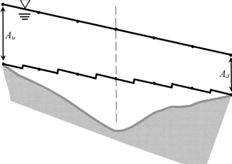
[image:6.612.309.478.409.476.2]Although we are focused on the momentum equation, for completeness we will start with continuity. The general ar-rangement of the control volume for an irregular channel and the vectors used in the following discussion are illustrated in Fig. 1. Applying only the incompressibility approximation for a uniform-density fluid, the volume-integrated continuity equation is
∂V ∂t +
I
S
uknkdA=SV, (14)
where the Einstein summation convention is applied on re-peated subscripts,uk is a vector velocity,nkis a unit normal
vector defined as positive pointing outward from a control volumeV, andSVis a volume source (SV<0 for a sink).
A semi-discrete finite-volume representation of continuity can be directly written as
∂Ve
∂t =Qu−Qd+qeLe, (15)
whereQandLrepresent the flow rate and element length, and subscripts “e”, “u”, and “d” denote characteristic val-ues for the control-volume element, nominal upstream face, and nominal downstream face, respectively. Here we use the nominal flow direction as the global downhill direction of the channel that is assigned at the network level. The average lat-eral inflow per unit length isqe, and a flowQ >0 is from the upstream to downstream direction. Reversals of flow from the nominal flow direction are handled withQ <0.
4.2 Momentum
The control-volume form of the Navier–Stokes momentum equation in a direction defined by unit vectorˆiin a Cartesian frame is
∂ ∂t
Z
V
uˆidV+ I
S
uiˆuknkdA+
1
ρ
I
S
pˆiknkdA
=
I
S
ν∂uj ∂xk
ˆ
ijnkdA+
Z
V
gˆidV , (16)
whereuˆi is a velocity vector component in theiˆ direction (i.e., the direction that is a priori of interest),uk represents
velocity components along Cartesian axes, the component of the gravity vector in theiˆdirection isgiˆ, the kinematic vis-cosity is ν, and p represents the thermodynamic pressure. Note that this formulation can be related to any arbitrary Cartesian axes. In many common derivations,iˆis approxi-mated as coincident with anxaxis that is a horizontal vector in the streamwise direction. In the following, we will show that this approximation is not required. Instead, we treat this as a simplification that can be applied to the final equation form.
4.3 Advection terms
Theiˆdirection for momentum, Eq. (16), is a vector associ-ated with theuˆivelocity, which is not necessarily coincident with the normal vectornkat a flux surface of a finite volume
Figure 1.General arrangement of control-volume element (Ve) and its neighbors for the irregular channel. Unit normal vectorsnkare always
perpendicular to cross-sectional areas (Au,Ad) and pointing outward from control volume. The element length (Le) is measured along the
channel. Unit vectors iˆk are coincident with the free-surface slope in the streamwise direction and can be defined as local continuous functions. The velocity vectorukis approximated as parallel toiˆk. The angle measured fromnktoiˆkisψ. The free-surface elevationsηu, ηe, andηdare cross-section uniform elevations at the upstream face, for the element center, and the downstream face, respectively. Note that
volume isV throughout the derivations withuandUused for continuous and spatially averaged velocities, respectively.
as the nominal downstream direction along the channel cen-terline described by a vector that lies along the free surface, as illustrated in Fig. 1. Thus, this vector is local (as opposed to being forced into coincidence with a Cartesian axis) and changes along the channel with the slope of the free surface. It follows that a discrete control-volume formulation devel-oped from Eq. (16) can be globally exact asVe→0. In con-trast, a derivation that takes ˆi as a vector in the horizontal direction has a momentum conservation error proportional to cosψ, whereψis an angle between the horizontal vector and the free surface; such an error does not vanish asVe→0 unless the free surface is flat across the length of the ele-ment. This idea helps illustrate one of the subtle implications of the Godunov approach in which the channel is imagined as having a piecewise flat free surface: cosψ=1 is then an identity within the approximation of the physics rather than an approximation within the mathematics.
For Eq. (16), the upstream element face is required to be vertical and normal to the smooth channel centerline in a hor-izontal plane, as illustrated in Fig. 1. The free surface at the centerline has an angle ofψ (x)to the horizontal so that the discrete nonlinear momentum term in theiˆdirection across the upstream face is formally
Z
Au
uiˆuknkdA= βQUˆi
u, (17)
whereQis the flow rate,Uiˆis the average streamwise veloc-ity over the cross-sectional area, the “u” subscript indicates the upstream face (rather than vector components), andβ is the momentum coefficient for the streamwise velocity, de-fined as
β≡ 1
A Uˆi 2
Z
A
uiˆ 2
dA. (18)
Note that the only approximation in the convective term of Eq. (17) is that the streamwise velocity is parallel to the free surface. However, the interpretation of theuiˆanduknkterms
may not be obvious, so further explanation is provided in Appendix A. For notational convenience, it is useful to let
U≡Uˆi. However, sinceQ=A R
uknkdA, strictly speaking
this requires an unconventionalQ=AUcosψ. If the chan-nel is straight and the free surface is linear so that the up-stream face is parallel to the downup-stream face and there is a single value ofψ, it follows that an exact finite-volume inte-gration of the nonlinear advection term is
I
S
uˆiuknkdA= −βuQuUu+βdQdUd−Me, (19)
For the more general case where the channel is curved be-tween the upstream and downstream faces and the free-surface gradient changes (as in Fig. 1), the above integra-tion becomes an approximaintegra-tion that is only exactly satisfied in the limit as the control-volume length goes to zero. For present purposes, the use of a gradually varying streamwiseˆi direction implies that pressure is perfectly redirecting mo-mentum through bends and aligning the momo-mentum with the free surface. These are (generally) unstated approximations used in common 1-D SVE formulations. However, it should be noted that this perfect momentum redirection is not pre-cisely correct; e.g., secondary circulation in bends affects bed shear, velocity distribution, and frictional losses (Blanckaert and Graf, 2004). Arguably, losses associated with flow redi-rection in channel bends and/or rapid changes in the free-surface gradient should be built into the frictional term in any model. Unfortunately, this remains a relatively poorly studied area at the interface of hydrology and hydraulics. The curva-ture effects on the equations can be written as perturbation terms that relate the channel width to the radius of curvature (Hodges and Imberger, 2001; Hodges and Liu, 2014), but these ideas have yet to be exploited in developing curvature effects in SVE numerical models.
4.4 Pressure decomposition
For the pressure term in Eq. (16) we follow the traditional approach for incompressible flows of defining a modified pressure (Pe) that includes the gravity term, which requires
e
P =p+ρgz. More formally we define 1
ρ
I
S
e
PˆiknkdA≡
1
ρ
I
S
piˆknkdA−
Z
V
giˆdV . (20)
The surface integral for the modified pressure decomposes into integrations over the upstream cross section (Au), the downstream cross section (Ad), the channel bottom (AB), and the free surface (Aη) as
1
ρ
I
S
e
PˆiknkdA=
1
ρ
Z
Au e
PiˆknkdA+
Z
Ad e
PˆiknkdA
+
Z
AB e
PiˆknkdA+
Z
Aη
e
PˆiknkdA
. (21)
Note thatABincludes both the bottom and side walls (if any). The above is an exact pressure term without imagining the geometry to be rectilinear or that the free surface has any simplified shape. The only geometric requirement of the vol-ume is that facesAuandAdmust be vertical planes that cut across the channel, which is necessary for consistency with the convective term. The first simplification we can introduce is to approximate the free surface as uniform at any cross sec-tion. The slope of the free surface is then coincident with the
ˆ
i(x)vector everywhere, which is aligned with the free sur-face at the channel centerline. With the free sursur-face aligned withˆi(x), the modified pressure is normal to the free surface everywhere and cannot contribute to the streamwise momen-tum (which we have defined as parallel toˆi(x)in deriving the advection terms, above). It follows thatPeiˆknk is identically
zero at the free surface and the last term in Eq. (21) vanishes. 4.5 Piezometric and non-hydrostatic pressure
It is convenient to introduce a decomposition of the modi-fied pressure (eP) into a piezometric pressure (P) and non-hydrostatic pressure (P˘), where only the latter is nonuni-form over a cross section. The non-hydrostatic pressure is defined by the difference between the modified pressure and the piezometric pressure:
˘
P (x, y, z)≡P (x, y, z)e −P (x). (22) The piezometric pressure is formally the sum of the hydro-static pressure and the gravitational potential at any pointz
for zb≤z≤η, which provides P (x, y, z)≡ρg[η(x, y)−
z] +ρgz=ρgη(x,y). For the SVEs, the free-surface eleva-tion can be considered uniform over the channel breadth (i.e., neglecting cross-channel tilt in channel bends). It follows that the piezometric pressure is
P (x)=ρgη(x), (23)
which is uniform over a vertical cross section. The non-hydrostatic pressure was neglected by de Saint-Venant and arguably should be neglected in any 1-D momentum equa-tion bearing his name. However, for completeness we retain the non-hydrostatic pressure terms in the derivation below but neglect them in discrete forms of the piezometric pres-sure terms in Sect. 5.
4.6 Pressure on flow faces
To further simplify the first two pressure terms in Eq. (21), we defineψ (x) as the angle between a horizontal line and the free surface,η(x), measured clockwise positive from the horizontal line pointing downstream. Thus, theiˆ vector is generally at an angle ±ψ (x) and pointing in the nominal downstream direction, as shown in Fig. 1. At the upstream cross section the pressure force without approximations is Z
Au e
PiˆknkdA= −(cosψu) Z
Au e
P (x, y, z)dA, (24)
where subscript “u” indicates values at the upstream cross section. Similarly, the downstream cross section provides Z
Ad e
PiˆknkdA= +(cosψd) Z
Ad e
Figure 2.Pressure decomposition to obtain streamwise contribu-tion.
where subscript “d” indicates values at the downstream cross section. Note that, in the above and in the following deriva-tions, the ubiquitous 1/ρ coefficient of all pressure terms are omitted for clarity. Introducing the piezometric and non-hydrostatic pressure split of Eq. (22) provides
Z
Au e
PˆiknkdA= −PuAucosψu−(cosψu)
Z
Au ˘
P (x, y, z)dA, (26) Z
Ad e
PˆiknkdA= +PdAdcosψd+(cosψd)
Z
Ad ˘
P (x, y, z)dA. (27)
Note that using the piezometric pressure instead of the hy-drostatic pressure ensures that the only term requiring dis-crete integration at the upstream and downstream surfaces is the non-hydrostatic pressure. That is,P Acosψisnotan ap-proximate integral whose adequacy depends on simplifying assumptions in geometry (as is the case for integrals of hy-drostatic pressure in the Cunge–Liggett form) but is instead an exact integration of piezometric pressure for any cross-section shape.
4.7 Pressure on bottom topography
The third pressure term in Eq. (21) is more challenging than the pressure on the flow faces as the bottom surface nor-mal (nk) varies with irregular topography. Hence, the local
piezometric pressure contribution in the streamwise direc-tion (iˆ) at any position (x,y) depends not only on the local water surface elevation but on the local irregularities in to-pography. It follows that integrating this term over a control volume requires some approximation of the subgrid topog-raphy. To arrive at a simpler formulation we note that the pressure acting normal to an arbitrary topography element at position (x,y) with surface normalnkwill have force
compo-nents that can be resolved along a set of local Cartesian axes. One axis is taken along a topography slope angle ofθ that lies in the same vertical plane as the streamwise directioniˆ,
Figure 3.Stair-step approximation for pressure along the bottom where tread is parallel to the free surface and riser is perpendicular for linear slopes of both the bottom and free surface.
as illustrated in Fig. 2. We can imagine Fig. 2 as an infinites-imal slice across a channel of irregular topography such that a series of these slices (with differentθ) can represent any cross-section shape. The second local Cartesian axis is taken within the same vertical plane but perpendicular to the axis defined byθ. The third axis, perpendicular to the other two, is necessarily horizontal and in the cross-channel direction (out of the page in Fig. 2). We are interested only in how the topography contributes to pressure in the streamwiseiˆ direction, so by definition the cross-channel pressure compo-nent is irrelevant. This approach is entirely consistent with changes in depth across the channel and changes in breadth along the channel – both merely alter the surface normal vec-tornk that is resolved into the local Cartesian system based
on the local slope direction ofθ.
To isolate the pressure forces acting in theiˆ streamwise direction, as a conceptual model we can imagine the to-pography in the infinitesimal slice of Fig. 2 replaced with a set of m=1 . . .N stair steps, where the treads are lo-cally parallel to the free surface and the risers are normal to the free surface, as illustrated in Fig. 3. Clearly, asN→ ∞
[image:9.612.50.284.69.224.2]Figure 4. Three-dimensional conceptual model of stair-step riser (gray) as a 2-D planar area of AR(m) separating two tread areas
(blue, red).
Figure 5.Conceptual model of piecewise linear approximation of nonlinear free surface and stair-step approximation of nonlinear to-pography with the cross-sectional area monotonically increasing. Pressure on the discrete riser areaAR(m)is locally aligned with the
free-surface slope directly above. The vertical scale and thus the tilt ofAR(m)are exaggerated for illustrative purposes.
topographic pressure force in the streamwise direction. As the brick dimensions go to zero the continuous topography is obtained.
Since the stair-step treads are (by definition) normal to the modified pressure above, it follows that the only pressure contributions to the momentum in the streamwiseiˆdirection are on the risers, with individual areasAR(m)form=1 . . .N
stair steps. Because the pressure contribution for increasing cross-sectional area (i.e., steps down as in Fig. 3) will be opposite of the pressure contribution for decreasing cross-sectional area (i.e., steps upward), it is convenient to intro-duce a functionγ(m)= ±1 to account for the change in sign
needed for the direction of the pressure force. We can for-mally defineγ(m)≡ ˆikjˆkat stepmwherejˆkis the normal unit
vector (pointing outwards) from theAR(m)riser, as shown in
Figure 6.Conceptual model of piecewise linear approximation of nonlinear free surface and stair-step approximation of nonlinear bot-tom with cross-sectional area increasing fromAuto the center and
then decreasing from the center toAd. Pressure on the discrete riser
areaAR(m) is locally aligned with the free-surface slope directly
above. The vertical scale and thus the tilt ofAR(m) are
exagger-ated for illustrative purposes. Note that the topography is identical to Fig. 5 but the stair steps are different due to the alteration of the free surface.
Figs. 5 and 6 for two different nonlinear water surface pro-files over identical bottom topography. It follows that Z
AB e
PiˆknkdA≈ − N
X
m=1
γ(m)
Z
AR(m)
e
P (x, y, z)dA. (28)
The above summation can be written as an integral over the lengthLof the finite-volume element asN→ ∞.
Z
AB e
PiˆknkdA= −
Z
L
γ (x)
Z
AR(x) e
P (x, y, z)dAdx, (29)
whereγ (x)= ˆikjˆk is the continuous counterpart to the
dis-creteγ(m). Note that this conceptual model is valid even for
non-monotonic behavior of the riser area (e.g., Fig. 6) as long as theAR(m)’s are continuous and smooth asN→ ∞.
However as discussed in Sect. 5, below, extremes of non-monotonic behavior can make it difficult to create a consis-tent discrete equation for the topographic pressure for a con-trol volume of finite size.
For further simplification, it is convenient to introduce the piezometric/non-hydrostatic splitting of Eq. (22) where, by definition, the piezometric pressure is uniform over a vertical cross section (e.g., a stair-step riser). LetP(m)represent the
piezometric pressure at themstair-step riser with areaAR(m)
[image:10.612.50.285.266.439.2]Z
AB e
PiˆknkdA= −
Z
L
γ (x)P (x)AR(x)dx
−
Z
L
γ (x)
Z
AR ˘
P (x, y, z)dAdx, (31)
which is a complete representation of the topographic pres-sure contribution to streamwise momentum in terms of the effective riser areas – i.e., the contribution based on the com-ponent of the bottom normal projected in the streamwise di-rection.
The stair-step conceptual model andARallow us to con-sider the pressure effects along the iˆ direction due to the changing cross-sectional area of the channel without intro-ducing the separate force terms I1 and I2 of the Cunge– Liggett form of the SVEs. An interesting part of this model is thatAR(x)over a control volume is a function ofboththe lo-cal bottom topography and the lolo-cal free-surface slope. That is, comparing Figs. 5 and 6 we see thatAR(m)riser areas are
different, despite the identical bottom topography. Returning to our idea that 3-D topography can be represented by dis-crete bricks, we can imagine each brick is pinned on an axis that allows it to locally rotate to different angles so that the upper surface is always parallel to the free surface. Again, the continuous topography is recovered as the brick size goes to zero, but the brick rotation allows the representation of the different topography effects that are caused by the interac-tion between the change in relainterac-tionship between the down-stream vector, ˆi, and the bottom normal vector as the free-surface profile evolves. Thus, AR is a dynamic representa-tion of the interacrepresenta-tion between the free-surface gradient and bottom topography that controls the effective along-stream pressure gradient of converging or diverging flow areas.
In theory, we might directly computeR
P ARdxover a con-trol volume; however, it seems likely that direct discretiza-tion of subgrid topography could cause unbalanced momen-tum source terms. In effect, computing R
P ARdx has the same complexity as computing the I1 or I2 terms of the Cunge–Liggett form and gains us little. Thus, it is useful to consider limiting approximations that can be developed from examining the geometry of Figs. 3 and 5. In the simplest case
a similar geometric identity:
A(m−1/2)cosψ(m)−A(m+1/2)cosψ(m)=AR(m), (33)
whereA(m±1/2)cosψ(m) represents the areas normal to the
free surface on the upstream and downstream edges of the
mpiecewise linear stair step. For the nonlinear free surface and/or topography over adjacent linear stair steps there is a discontinuity of the treads for adjacent steps as cosψ(m−1)6=
cosψ(m), so the discrete summation of the stair-step areas
over a control volume provides an approximation rather than an identity:
Adcosψd−Aucosψu≈
N
X
m=1
AR(m). (34)
However, in the limit as N→ ∞ we have a single value of cosψat any point along a smooth free surface so that the continuous form provides an identity:
Adcosψd−Aucosψu= Z
L
AR(x)dx. (35)
To generalize the above forAd< Au, we can use theγ (x)=
±1 that was introduced for the pressure direction in Eq. (29). Values ofγ (x)= +1 indicate that the cross-section area is increasing across locationx in the streamwise direction (as in Figs. 3 and 5), whereasγ (x)= −1 indicates that the cross-sectional area is decreasing (as in the latter portion of Fig. 6). It follows that
Adcosψd−Aucosψu= Z
L
γ (x)AR(x)dx (36)
is an identity that should be satisfied for any control volume where the bottom topography and free surface are continuous and smooth. Note that if Fig. 3 is imagined as one of many infinitesimal slices (with varyingθ) that make up a channel cross section, it should be obvious that Eq. (36) also applies for a finite volume with irregular (smooth) topography.
To handle the integration of AR(x) in the piezometric pressure term of Eq. (31), we introduce a quadrature func-tionλ(x), defined as
λ(x)≡ γ (x)AR(x) Adcosψd−Aucosψu
Note that with Eq. (36), this implies the identity Z
L
λ(x)dx=1. (38)
Using the above in the first term on the RHS of Eq. (31), we obtain
Z
L
γ (x)P (x)AR(x)dx=(Adcosψd−Aucosψu)
×
Z
L
P (x)λ(x)dx. (39)
Thus, the introduction ofλallows us to extract a multiplier from the control-volume integral of the bottom pressure. As a result, λ(x) is merely a distribution, or weighting func-tion, for integration ofP (x). The full bottom pressure term, Eq. (31), can be written as
Z
AB e
PiˆknkdA= −(Adcosψd−Aucosψu) Z
L
P (x)λ(x)dx
−
Z
L
γ (x)
Z
AR ˘
P (x, y, z)dAdx. (40)
Note thatλweighting cannot be readily applied to the non-hydrostatic term because the non-non-hydrostatic pressure on the bottom has spatial distributions in both the vertical and cross-channel directions that cannot be assumed to be negligible; hence we cannot passP˘ through theARintegration as was done in Eq. (30) forP.
We can think ofλ(x)as a weighting function of the con-ceptual stair-step riser areas over the control-volume length, which controls where the piezometric pressure gradients have their greatest effect. For example, in Fig. 3 the stair-step risers are uniformly distributed such that we can useλ(x)= L−1, which meets the identity requirement of Eq. (38). In contrast, Fig. 5 implies thatλ(x)is perhaps a quadratic func-tion. Figure 6 presents a challenge as λ(x) should reverse in sign between the upstream and downstream faces. A key point in the new finite-volume derivation is thatλ(x)controls the representation of the free surface and bottom topography within a volume. This can be contrasted to the Godunov ap-proach that uses piecewise linear approximations for both the bottom and free-surface elevations (see Sect. 3). Several dis-crete approaches to the approximation ofλ(x)are examined in Sect. 5, although the full consequences and utility of the
λapproach will require more extensive investigation for both theoretical limitations and practical discretization schemes.
4.8 Combining pressure terms
In summary, the pressure terms of Eq. (21) can be written using Eqs. (26), (27), and (40), resulting in
1
ρ
I
S
e
PˆiknkdA= −
1
ρAuPucosψu+
1
ρAdPdcosψd −1
ρ(Adcosψd−Aucosψu)
Z
L
P (x)λ(x)dx
−cosψu ρ
Z
Au ˘
P (x, y, z)dA
+cosψd ρ
Z
Ad ˘
P (x, y, z)dA
−1 ρ
Z
L
γ (x)
Z
AR ˘
P (x, y, z)dAdx, (41)
where the last three terms are the non-hydrostatic pressure effects that are typically neglected in the SVEs.
4.9 Viscous term
The remaining term in Eq. (16) is the viscous term, which is treated as an empirical function in all but the most highly resolved models of simple systems – note that Decoene et al. (2009) provide a comprehensive and rigorous approach for friction that has not yet been fully considered in SVE mod-els. For the present purposes, we will retain the simple fric-tion slope form with an assumpfric-tion of uniform behavior over space, i.e.,
I
S
ν∂uj ∂xk
ˆ
ijnkdA= −g
Z
Ve
Sf(x)dV ≈ −gVeSf(e), (42)
whereSf(e)is the average friction slope over the control
vol-umeVe.
4.10 Finite volume for momentum
AR
whereUeis the element velocity in the streamwise direction,
Ve is the element volume, and the relationship between U andQis given by
Q=AUcosψ. (44)
Note thatQ >0 andU >0 imply flow in the nominal down-stream direction, whereas Q <0 andU <0 imply flow in the nominal upstream direction. At this point we have troduced only four approximations: (1) uniform-density in-compressibility, (2) the effect of channel curvature is either negligible or handled in an empirical viscous term, (3) the cross-channel variability in the free-surface slope is negligi-ble, and (4) a friction-slope model can be used to represent integrated viscous effects over a control volume. In addition we have a geometric restriction that the upstream and down-stream control-volume cross sections must be vertical planes that are orthogonal (in the horizontal plane) to the mean flow direction.
For convenience in exposition, for the remainder of this paper we will apply the hydrostatic approximation (P˘=0) along with approximations for the small slope (cosψ≈1) and uniform cross-section velocity (β≈1). Furthermore, we will limit our focus to flows without lateral momentum sources (Me=0). These simplifications allow us to focus at-tention on the pressure source term, which is the primary new contribution in this derivation. The resulting simplification of Eq. (43) can be presented with conservative terms on the LHS and source terms on the RHS as
∂
∂t(UeVe)− Q2u Au
+Q
2 d
Ad
−gAuηu+gAdηd
=g (Ad−Au) Z
L
η(x)λ(x)dx−gVeSf(e), (45)
where definition of piezometric pressure, Eq. (23), is used to substituteP =ρgη. A more formal finite-volume integral presentation would be
If we substitute geometric identities η≡H+zb and S0≡
−∂zb/∂x, we see that the above becomes identical to Eq. (8). Thus, our finite-volume derivation is exactly consistent with the commonly used differential SVEs that is posed usingS0. However, from Eqs. (45) and (47) we see that the free-surface source term in the differential form,gη∂A/∂x, is related to the more interesting integral source term in the finite-volume form:
g (Ad−Au) Z
L
η(x)λ(x)dx.
This piezometric pressure term can be thought of as the in-tegrated free-surface/topography effects over a control vol-ume of finite size. It is clear that this term collapses to
gη∂A/∂x as L→0, but the integral form cannot be read-ily inferred from the differential form. Through approxima-tions of this integral term we can obtain a variety of different finite-volume forms of the SVEs, as outlined in the following section.
5 Approximate finite-volume forms of the SVEs 5.1 General form
We are interested in approximate forms of the finite-volume SVEs that arise from discretization choices in the integral pressure source term derived above, so for exposition it is convenient to start from the approximate form in Eq. (45) withVe=AeLeandQe=AeUe. These approximations can be readily reversed to provide a more complete equation, but the simple form for further analysis is
Le∂Qe ∂t −
Q2u Au
+Q
2 d
Au
−gAuηu+gAdηd=Te−gVeSf(e), (48)
where Te is the source term for integrated free-surface/topography pressure effects obtained from the RHS of Eq. (45):
Te≡g (Ad−Au) Z
L
Note that the LHS of Eq. (48) is discretely conservative in that a summation over all elements will cause all the LHS terms to identically vanish except for the∂/∂tand boundary conditions. Thus, the RHS shows the source terms; i.e., the traditional friction term and a term representing nonlineari-ties in the free surface interacting with topography can cre-ate and destroy momentum. The system is inherently well-balanced as discussed in Sect. 3, as long as Te identically balances the spatially integrated piezometric pressure gradi-entgAdηd−gAuηufor a flat free surface.
Equation (49) admits a wide variety of approximate equa-tions, depending on the form chosen for the quadrature ofη(x)andλ(x)over the length of a finite volume. Arguably, a simple finite-volume discrete method will have three val-ues ofηthat characterize a control volume:ηu,ηe, andηd, as illustrated in Fig. 1. Different numerical methods can be con-structed by using different approximations concon-structed from these three values. Herein, we cannot exhaustively investi-gate the variety of options and so will focus on the most obvi-ous candidates, which are polynomials of orders 0 through 2. The zero-order polynomial is an approximation of η(x)as a uniform value over the element length (e.g., as in the Go-dunov conceptual model, discussed in Sect. 3) – which could be simply represented by η(x)=ηe so that the face values of ηd and ηu are ignored. Note that even this choice has alternate forms – a slightly different scheme could be con-structed usingη(x)=(ηu+ηd)/2, which is also uniform but ignoresηe. A first-order polynomial forη(x)implies a linear free-surface slope across the element, which might be rep-resented by a slope from ηd toηu. A second-order polyno-mial implies a quadratic curvature to the free surface that can pass smoothly throughηu,ηe, andηd. Clearly this idea could be extended to cubic splines by including adjacent control-volume values. Beyond these polynomials there are other options that might be suitable. For example, we could use the three discreteηvalues to provide piecewise linear slopes from ηu toηe and ηe toηd. The open-ended nature of the
η(x)discretization should allow future development of a va-riety of finite-volume forms that can be easily demonstrated to be well-balanced and consistent with the above deriva-tions.
By its definition in Eq. (37) with constraint Eq. (38), the weighting functionλ(x)is an abstraction of the topographic pressure distribution over a finite volume, which is affected by both topography and the local slope of the free surface, as illustrated in Figs. 3, 5, and 6. Theλ(x)is more complicated and abstract thanη(x)because the free-surface elevation is approximated as uniform across the channel at any x loca-tion, butλ(x)represents the integrated effect of complex 3-D topography, e.g., theAR(m)stair step as illustrated in Fig. 4.
The key point is that theλ(x)weighting function has an inte-gral constraint ofR
[image:14.612.310.546.66.232.2]λdL=1 because the change in the cross-sectional area over the control-volume flux faces, Ad−Au, has already been extracted from the integral ofP ARthrough Eq. (39). A comparison of Figs. 5 and 6 shows thatλ(x)isnot
Figure 7.Non-monotonic stair steps of the cross-sectional area with linear monotonic free surface. The dashed gray line is where the cross-section area reverses from increasing to decreasing.
independent ofη(x)and hence arguably should be a moder-ator between the static topography and the dynamics of the free surface. However, the development ofλ(x,t )forms that are dynamically dependent onη(x,t )is beyond the scope of the present work. Herein, we appeal to Occam’s razor and note that the simplest λ(x) that satisfies the integral con-straint isλ(x)=L−1e , whereLeis the control-volume length, illustrated in Fig. 1. This choice ofλ(x)is a zero-order poly-nomial implying the stair steps are uniformly distributed over the element, as illustrated in Fig. 3. Clearly, for the nonlinear cases in Figs. 5 and 6, this form ofλ(x)is an approxima-tion that reduces the nonlinear interacapproxima-tion between the free surface and the topography. Arguably, this is consistent with a discrete scheme using a single-valued geometry function such asηe=f (Ve)that neglects the effect of the free-surface slope on the relationship between volume and surface eleva-tion. Note that because theAd−Auarea is already extracted from the integral, usingλ(x)=L−1e ensures that theTeterm is exact at the linear limit and a bounded approximation for nonlinear interactions. That is, withλ(x)=L−1e it follows that
Te=
g (Ad−Au)
Le Z
L
η(x)dx≤g (Ad−Au)max(η(x)) .
Thus, the largest possible value for theTeterm is based on the maximum piezometric pressure over the control volume acting on the difference between upstream and downstream areas.
Figure 8.Approximated finite-element cross-section characteristics using λ(x)=L−1e for non-monotonic topography in Fig. 7. The
dashed gray line is where the cross-section area reverses from in-creasing to dein-creasing.
increases along the streamwise direction in the upper sec-tion and decreases in the lower secsec-tion, as shown in Fig. 7. Theλ(x)=L−1approach cannot represent the actual change in cross-section area but instead provides a linear trend be-tweenAuandAdas shown in Fig. 8. In contrast, if the con-trol volume in Fig. 7 were split into two separate volumes at the centerline (i.e., the dashed gray line), then the stair steps of Fig. 7 would be readily represented by the λ(x)=L−1
approximation as both control volumes would be monotonic. A comprehensive investigation of different forms forη(x)
andλ(x)in theTe term is clearly needed and will take sig-nificant future effort. For the present purposes, we exam-ine the simplest polynomial forms for η(x)in combination with the zeroth-order λ(x)=L−1. To provide insight into how a higher-order λ(x) discretization adds complexity in the derivation, we can derive a simple linear form ofλ(x)that depends only on topography and couples with a linear form ofη(x). Such aλ(x)is unlikely to be useful with a dynamic free surface but is illustrative of the complexity that can be developed with quadrature of even simple linear equations. We will use the nomenclatureTe(m,n)to designate anm-order
polynomial forη(x)and ann-order polynomial forλ(x). 5.2 TheTe(0,0)approximation
The simplest approximations arise by assuming uniform val-ues such thatη(x)≈ηandλ(x)≈L−1e , whereηis the aver-age water surface elevation over the element, and we recall thatRLλdx=1. It follows that
Te(0,0)≡g (Ad−Au) η. (50)
If we letηe≈η, then Eq. (48) can be written as
we obtain
Te(1,0)=g (Ad−Au) aL
2 +b
. (52)
A linear approximation is consistent with a free surface whereb=ηuanda= −(ηu−ηd)/L, so we obtain a finite-volume source term:
Te(1,0)=
1
2g (Ad−Au) (ηu+ηd) . (53) Note that the above implies products ofAdηd andAuηuin the source term that can be moved to the LHS as part of the conservative flux terms. SubstitutingTe(1,0)forTein Eq. (48) and redistributing terms provides
Le
∂Qe
∂t − Q2u Au
+Q
2 d
Au
−1
2gAuηu+ 1 2gAdηd
=1
2g (Adηu−Auηd)−gVeSf(e). (54) Thus, the model of a linear free surface and uniformλ(x)
serves to change the weighting of thegAηterms (from unity to 1/2) and provides a source term that contains only face values ofAandη, which is unlike Eq. (51) which requires an element approximation ofηe. Interestingly, the above finite-volume form doesnot have a differential representation as
L→0. That is, the free-surface differential source term in Eq. (47) is based on(Ad−Au)/L→dA/dxasL→0. How-ever, once we have chosen relationships forη(x) andλ(x)
and moved a portion of the source term into the fluxes, an at-tempt to create a differential out of our source term encoun-ters the form
lim
L→0
Adηu−Auηd
Le
,
Le
∂
∂t(HeUe)−HuU
2
u+HdUd2+ 1 2g
Hd2−Hu2
=g(Hd+Hu)
2 (zu−zd) . (55)
AsLe→0, andS0= −∂z/∂x, the above implies a conser-vative differential form of
∂H U ∂t +
∂ ∂x
H U2
+1
2g
∂H2
∂x =gH S0, (56)
which is commonly used in studies of simplified conservative forms (e.g., Bouchut et al., 2003; Hsu and Yeh, 2002). Thus theTe(1,0)is also consistent with prior differential forms.
5.4 TheTe(2,0)approximation
We can take this approach further by approximating the free surface as a parabola based on {ηu,ηe,ηd}, whereηe is a characteristic free-surface height at the center of the finite volume. Using η(x)=ax2+bx+c withx=0 at Au and
x=LatAdprovides
c=ηu, (57)
b= 1
L(−3ηu+4ηe−ηd) , (58)
a= 2
L2(ηu−2ηe+ηd) . (59)
Usingλ(x)=L−1results in
Te(2,0)=
g
6(Ad−Au) (ηu+4ηe+ηd) . (60) It is useful to multiply through and regroup terms so that
AdηdandAuηuare isolated. Where these terms are balanced, they can be moved to the LHS as conservative terms. Re-grouping provides
Te(2,0)=
g
6{Adηd−Auηu+Ad(ηu+4ηe)
−Au(4ηe+ηd)}. (61)
So our momentum equation can be written as
Le
∂
∂t(Qe)− Q2u Au
+Q
2 d
Ad
−5
6gAuηu+ 5 6gAdηd
=1
6g{Ad(ηu+4ηe)−Au(4ηe+ηd)}
−gVeSf(e). (62)
Once again, the specific representation ofη(x)λ(x)provides a modification of the coefficient of thegAηterms in the con-servative fluxes and sets the form of the non-concon-servative source term. This form does not appear to readily reduce to any differential form that is previously seen in the literature and thus provides an interesting new avenue for investiga-tion.
5.5 TheTe(1,1)approximation
The above forms used a uniformλ(x)=L−1. We can readily extend the concept to analytical forms ofλ(x), although it is not clear that such increasing complexity will yield an advan-tage in the design of a numerical model. Theλ(x)function is a weighting function that reflects the distribution of the bot-tom elevation stair steps, as described in Eq. (4). The only restriction onλ(x)is that it must integrate to unity overLe. Physically, as illustrated in Figs. 3, 5, and 6, theλ(x)should be a function ofη(x)as well as the topography. However, we do not (as yet) have a good working framework for a dy-namic representation ofλ(x,η). Thus, to illustrate the com-plexities that arise with a nonuniformλ(x), herein we will simply analyze a somewhat arbitrary static linear relationship whereλ(x)=αz(x), wherezis the bottom elevation andαis a scaling constant to ensureR
L
λdx=1. We introduce linear approximations of the bottom asz(x)=Ax+Band the free surface asη(x)=ax+b. We can write these approximations as
z(x)= −1
L(zu−zd) x+zu, (63)
η(x)= −1
L(ηu−ηd) x+ηu. (64)
UsingR
L
αz(x)=1, it can be shown that
α= 2
L (zu+zd)
. (65)
Using Eq. (49), a quadrature problem can be presented as
Te(1,1)
g (Ad−Au)
=α
Z
L
z(x)η(x)dx= 2 L (zu+zd)
×
Z
L
−1
L(zu−zd) x+zu
×
−1
L(ηu−ηd) x+ηu
dx. (66)
After some algebra, we find
Te(1,1)
g (Ad−Au)
=2ηuzu+ηuzd+ηdzu+2ηdzd
3(zu+zd)
. (67)
Unfortunately, for the above form we cannot use the redis-tribution trick to split Te and move a portion to the LHS of Eq. (48). The problem is that any split term will have
purposes and isnotrecommended for use in any numerical scheme. ThisTe(1,1) is predicated on an assumed weighting
of λ(x)=αz(x), which does not have a physical linkage to specific cross-section geometry or expected flow conditions. 5.6 Summary of approximate forms
TheTe(0,0),Te(1,0),Te(2,0), andTe(1,1)approximations all
fol-low a similar form
Le
∂Qe
∂t − Q2u Au
+Q
2 d
Ad
−gAuηu(1−δu)+gAdηd(1−δd)
=Ke(m,n)−gVeSf(e), (69)
where 0≤δuandδd≤1 are fixed coefficients andKe(m,n)is
a time–space-varying topographic source term, whose exact forms are determined by the approximations used forTe. This form was suggested in Sect. 2 with Eq. (9) based on a philo-sophical argument of moving as much of the RHS source terms as possible to the conservative LHS flux terms. The key point for future work is that these forms (with the ex-ception ofKe(1,1)) are relatively straightforward in their
rep-resentation of values that are the natural elements of a SVE computational model for river networks and urban drainage. This approach eliminates the need for estimating or comput-ing theI1andI2of the Cunge–Liggett conservative form and replaces them with the simple cross-sectional area term and aKethat is computed from discrete values ofηandA. Values for δu,δd, andKefor these forms are presented in Table 2. Examination of the above leads to the conclusion that the use of any polynomial representation of η(x)withλ(x)=L−1
will produce aKe(m,0)source term that will exactly balance
the piezometric pressure terms of the LHS when the free sur-face is flat; e.g.,ηu=ηe=ηd. Thus, these schemes are in-herently well-balanced as discussed in Sect. 3. Furthermore, for these cases the source terms will be Lipschitz smooth as long as the solution variables are smooth.
6 Summary and discussion
The conservative differential form of the non-hydrostatic version of the Saint-Venant equations, simplified from the derivation in Sect. 4, can be written as
∂AU ∂t +
∂ ∂x
"
βAU2+gAη+ ˘ P ρ
# cosψ
!
=gη∂A
∂xcosψ+
1
ρ
Z
AR ˘
P (z)dA−gASf+me, (70)
wheremeis the source and sink of momentum from lateral fluxes per unit length (i.e.,MeL−1). This equation is similar to previous work but includes both non-hydrostatic terms and effects of free-surface slope (cosψ) that are often neglected. The key contribution of the present work is the semi-discrete, conservative, finite-volume form that corresponds to the dif-ferential form above:
∂
∂t(UeVe)−βuAuU
2
ucosψu+βdAdUd2cosψd−gAuηucosψu
+gAdηdcosψd− cosψu
ρ Au ˘ Pu+
cosψd
ρ Ad ˘ Pd
=g (Adcosψd−Aucosψu) Z
L
η(x)λ(x)dx
+1 ρ Z
L
γ (x) Z
AR ˘
P (x, y, z)dAdx−gVeSf(e)+Me, (71)
[image:17.612.309.549.130.303.2]pressure gradients in the horizontal as absorbing and redirect-ing momentum along the curvredirect-ing channel. Thus a part of this term is, in effect, encapsulated within the approximation that allowsAuandAdto be cross sections that are not parallel.
The principal feature of the new finite-volume formula-tion is the topographic source term R
η(x)λ(x)dx that can be represented by analytical functions to approximate a smoothly varying free surface and its interaction with to-pography across the finite-volume element. Discrete poly-nomial representations of Rη(x)λ(x)dx are evaluated in Sect. 5, with the resulting topographic terms designated as Te(m,n) for an m-degree polynomial representingη and
an n-degree polynomial representing λ. In an approximate form, the Te(m,n) term is split into a δu(m,n) factor applied
togAuηuand a δd(m,n) factor applied togAdηd, which be-come part of the conservative flux terms. The remainder of the Te(m,n) becomes a Ke(m,n) source term in the
approxi-mate finite-volume form. Simpler conservative finite-volume forms that use the common approximations of the hydrostatic equations (P˘≈0) with small free-surface slope (cosψ≈1), uniform cross-sectional velocity (β≈1), and no momentum sources (Me=0) can be written as
Le
∂Qe
∂t − Q2u Au
+Q
2 d
Ad
−gAuηu 1−δu(m,n)
+gAdηd 1−δd(m,n)
=Ke(m,n)−gLeAeSf(e), (72)
where the discrete Ke andδ terms are shown in Table 2. It is worthwhile to compare the above to a finite-volume form derived using the Cunge–Liggett form of the SVEs, which could be written (using theI1andI2definitions) as
Le
∂Q ∂t −
Q2u Au
+Q
2 d
Ad
−g
Z
H (u)
(H−z)B(z)dz
+g
Z
H (d)
(H−z)B(z)dz=g
Z
L
Z
H
(H−z)∂B ∂xdx
+g
Z
L
A (S0−Sf)dx. (73)
Performance of the traditional scheme depends on the spec-ification forB(x,z)that defines the irregular bathymetry of the channel. Although the B(x,z)term is developed with-out any approximations, it is a nontrivial matter to simplify these terms to create practical computational forms for irreg-ular cross-section geometry. The source term on the RHS of the Cunge–Liggett form is effectively an integration of both variations in the channel topography and the water surface elevation over the volume – similar to the newTe– but
with-out a limiting constraint (i.e., ∂B/∂xis not inherently lim-ited in magnitude for irregular topography). Furthermore, the selection of B(x,z) for the RHS affects the integration on the LHS hydrostatic pressure term – thus obtaining a well-balanced source term that compensates forS0will also affect
the conservative flux terms. The λ(x)used to develop the
Keterm Eq. (72) serves a similar purpose to the source-term integral in the Cunge–Liggett form, but it provides a simple weighting function that can be analytically integrated with an approximation forη(x)and is inherently constrained such thatR
λdx=1 over a control volume. The other major dif-ference between the two approaches is that Eq. (73) usesS0 as a source term on the RHS of the equations, whereas in the new approach Eq. (72) dispenses with this artifice so that the source terms only include friction (which is guaranteed to damp momentum) and the portion of the topographic ef-fects that cannot be transferred into the conservativeδu and
δdterms.
There is a long history of the use of S0 in the source term in the SVEs, and it is indeed part of the author’s prior model (Liu and Hodges, 2014). However, the use ofS0with irregular geometry brings the problems of creating a well-balanced conservative scheme, as discussed in Sect. 3. Fur-thermore, the use ofS0in the source term requires the pres-sure term to be treated as the hydrostatic prespres-sure rather than the piezometric pressure, as shown in Sect. 4. Because the hydrostatic pressure is a function of depth, its integration over a cross-sectional area requires knowledge of the dis-tribution of depth across the channel – a significant com-putational complexity for irregular topography. In contrast, the integration of the piezometric pressure over a cross sec-tion is exactlyP Aand does not require knowledge of how depth is distributed across the channel. Other authors have noted similar problems: Schippa and Pavan (2008) derived a conservative differential form that retainedgI1 in the flux terms and removed S0 by showing that it could be com-bined with theI2source term as∂I1/∂xfor a uniform water level. It seems that the Schippa and Pavan (2008) differen-tial equation might be preferred to the approach proposed herein for high-resolution topography with small grid spac-ing (i.e., where we have confidence that the computation ofI1 is meaningful). However, at larger scales where geometric cross sections are broadly spaced and the computation ofI1 is questionable, the simplicity of usingAandη for piezo-metric pressure gradient terms is likely to be preferred. Other authors, notably Rosatti et al. (2011), have simply accepted
gA∂η/∂xas an unavoidable source term rather than dealing with the problems of obtaining a well-balanced method with the hydrostatic pressure.
SinceS0was not in de Saint-Venant’s original paper, how did it come to be commonly used in the Saint-Venant equa-tions? Arguably there are two sources associated with differ-ent simulation scales: (1) in hydrology the kinematic wave model providesS0=Sf, which leads to prioritization ofS0 as a hydraulic parameter; and (2) in mathematics the equa-tion
∂h ∂t +
∂hu