www.hydrol-earth-syst-sci.net/18/1549/2014/ doi:10.5194/hess-18-1549-2014
© Author(s) 2014. CC Attribution 3.0 License.
Hydrology and
Earth System
Sciences
Decomposition analysis of water footprint changes in a water-limited
river basin: a case study of the Haihe River basin, China
Y. Zhi, Z. F. Yang, and X. A. Yin
State Key Laboratory of Water Environmental Simulation, School of Environment, Beijing Normal University, Beijing, China
Correspondence to: Z. F. Yang (zfyang@bnu.edu.cn)
Received: 22 November 2013 – Published in Hydrol. Earth Syst. Sci. Discuss.: 2 December 2013 Revised: – Accepted: 18 March 2014 – Published: 6 May 2014
Abstract. Decomposition analysis of water footprint (WF)
changes, or assessing the changes in WF and identifying the contributions of factors leading to the changes, is im-portant to water resource management. Instead of focusing on WF from the perspective of administrative regions, we built a framework in which the input-output (IO) model, the structural decomposition analysis (SDA) model and the gen-erating regional IO tables (GRIT) method are combined to implement decomposition analysis for WF in a river basin. This framework is illustrated in the WF in Haihe River basin (HRB) from 2002 to 2007, which is a typical water-limited river basin. It shows that the total WF in the HRB increased from 4.3×10¹⁰m3in 2002 to 5.6×10¹⁰m3in 2007, and the agriculture sector makes the dominant contribution to the in-crease. Both the WF of domestic products (internal) and the WF of imported products (external) increased, and the pro-portion of external WF rose from 29.1 to 34.4 %. The techno-logical effect was the dominant contributor to offsetting the increase of WF. However, the growth of WF caused by the economic structural effect and the scale effect was greater, so the total WF increased. This study provides insights about water challenges in the HRB and proposes possible strategies for the future, and serves as a reference for WF management and policy-making in other water-limited river basins.
1 Introduction
A water footprint (WF) concept quantifies the water re-source consumption of human beings (Yang and Zehnder, 2007). The WF of a region is the volume of fresh water consumed during the production of goods and services con-sumed by the inhabitants in that region (Hoekstra et al.,
2011; Hoekstra, 2013) and is a useful guide for virtual wa-ter (VW) trade and wawa-ter management (Allan, 1998, 1999; Zhao et al., 2005; Hoekstra and Chapagain, 2007; Wheida and Verhoeven, 2007; Verma et al., 2009; Hoekstra et al., 2011; Mekonnen and Hoekstra, 2012; Zeng et al., 2012; Wang et al., 2013). Furthermore, the WF of a product or service is mathematically equal to its VW content, which means the water resources consumed in its production pro-cess (Allan, 1998; Hoekstra and Hung, 2002, 2005; Zhao and Samson, 2012; Chen and Chen, 2013; Vanham et al., 2013). The WF of an economic sector identifies total water resource consumption in the production process (Hoekstra and Chapagain, 2007).
It is important to assess yearly changes in the WF of a re-gion, identify the key economic sectors and factors leading to the changes, and quantitatively evaluate the contributions of those sectors and factors to the changes so that policy-makers and management can take water-saving actions for the eco-nomic sector or factor with the largest contribution; this is called the decomposition analysis of WF changes (Hoekstra et al., 2011; Zhang et al., 2012).
IO model can identify the direct and indirect WF contained in the final products of each sector (Chen, 2000; Dietzenbacher and Velázquez, 2007; Lenzen, 2009; Zhao et al., 2009, 2010; Zhang et al., 2011a, b; Wang et al., 2013). Second, it is nec-essary to assess quantitatively the yearly changes in WF and the contributions of key factors (Hoekstra and van den Bergh, 2003; Kondo, 2005; Zhang et al., 2012).
On the basis of the IO model, the structural decomposition analysis (SDA) model has been developed to analyze quan-titatively the contribution of each factor to the total change (Hoekstra and van den Bergh, 2003; Guo, 2010). The IO model and the SDA model are widely used in decomposi-tion analysis of WF changes: several previous studies have proved that these methods can decompose the WF changes and quantitatively show the contribution of each sector and factor (Kondo, 2005; Zhang et al., 2012).
Previous studies only focused on decomposition analysis of WF changes from the perspective of administrative gions, however, river basins are more important to water re-source management. A river basin is a natural geographic unit and an important carrier of human activities with a rel-atively complete eco-hydrological pattern (Haihe River Wa-ter Conservancy Commission, 2008; Zhao et al., 2010; Mao and Yang, 2012). Studying water resources at the scale of a river basin could better reflect the water resources situa-tion, and managing water resources from the perspective of a river basin is more reasonable (Chen et al., 2005; Schendel et al., 2007; Verma et al., 2009; Zhao et al., 2010; Feng et al., 2012). Decomposition analysis of WF changes from the per-spective of a river basin is important to water resource man-agement and policy-making, especially in a water-limited river basin.
The lack of homologous IO data is a barrier to implement-ing decomposition analysis of WF changes from the per-spective of a river basin. Decomposition analysis is based on the IO model, which requires an IO table (Hoekstra and van den Bergh, 2002; Zhao et al., 2010; Zhang et al., 2012), but the IO table for a river basin is usually unavailable be-cause official statistics are provided based on administrative unit. Moreover, the IO data for a river basin cannot be ob-tained by simply adding the data for administrative regions together because there are economic exchanges between re-gions, which could only be identified with difficulty, and may lead to double counting.
[image:2.595.310.540.62.233.2]This study bridges the gap in quantitative knowledge and implements the decomposition analysis of WF changes from the perspective of a river basin. A generating regional IO ta-bles (GRIT) method is introduced to compute the IO data for a river basin from the administrative units located in that basin. A branch of the SDA model called the weighted av-erage decomposition (WAD) method is used in this analysis because it is more accurate than other kinds of SDA mod-els (Dietzenbacher and Los, 1998; Li, 2004; Kondo, 2005; Zhang et al., 2012). To test its effectiveness, this GRIT-IO-WAD framework is illustrated with the example of the Haihe
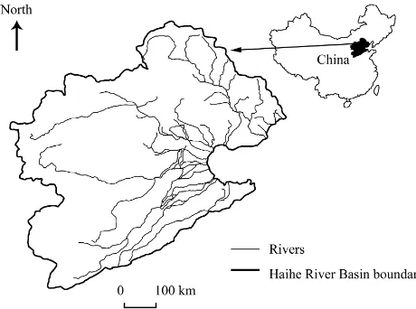
Fig. 1. Location of study area (adapted from website of Haihe
River Water Conservancy Commission http://www.hwcc.gov.cn/ pub/hwcc/static/szygb/gongbao2011/).
River basin (HRB), which is a water-limited river basin in northern China. The computation is made for the period 2002 to 2007, when the HRB experienced rapid industrial transfor-mation and economic growth, and the official data in this pe-riod is the latest available. This study analyzes WF changes in the HRB, and serves as a reference for water resource man-agement and policy-making in this and other water-limited river basins.
2 Methodology and material
2.1 Study area
2.2 GRIT-IO-WAD framework for WF
2.2.1 Computing the IO data with the GRIT method
The GRIT method, developed by Jensen et al. (1979), as-sesses the IO table for a region according to the IO tables of its sub-regions. Using the GRIT method, the IO table for a river basin can be obtained from the IO tables of the admin-istrative units located in the basin (Jensen et al., 1979; Zhao et al., 2010; Feng et al., 2012); thus the IO model and the WAD model could be used to quantify the WF from a river basin perspective.
To analyze the WF in the HRB in 2002 and 2007 by the IO method, the IO data for 2002 and 2007 on the river basin scale are necessary. Because official statistics are only pro-vided based on administrative units, in this study, the IO data from 2002 and 2007 are derived from the official IO tables of Beijing, Tianjin, and Hebei using the GRIT method. The GRIT method assumes that the proportion of intermediate products of economic sectors in a river basin is similar to that at the national level, and the proportion of the economic con-tributions of each administrative unit in the river basin equals the proportion of their land in the scope of the river basin (Jensen et al., 1979; Zhao et al., 2010; Feng et al., 2012). Even with these assumptions, the model has enough accuracy to be treated as a reflection of the real world (Jensen et al., 1979; Zhao et al., 2010; Feng et al., 2012). We use a series of mechanical steps to modify the national and administrative IO data to their equivalents in the HRB as follows:
First, the total output of each sector in the HRB is calculated:
T O= [pi] = [ηBpiB+ηtpti+ηHpiH], (1) where T O (RMB) is the vector of monetary total output in the HRB (n×1 dimensional vector;nis the number of sectors), whose element, pi, (RMB) is the output of
sec-toriin the HRB; ηB,ηt, andηH are the proportion of the land of Beijing, Tianjin, and Hebei in the scope of the HRB, which equates to 100 % in this study. pBi ,pit, and pHi are the total outputs of sectorifor Beijing, Tianjin, and Hebei, respectively.
Second, the matrix of intersectoral transactions of each sector in the HRB is calculated:
A= [aij] = [aijN×Lij] (2)
bij=aijN×(1−Lij) (3)
Lij= pi/P
i pi
piN/P
i
piN, (4)
where A is the direct consumption coefficient matrix (n×n
dimensional matrix) in the IO table, whose element,aij, is
the direct consumption coefficient, which means the mone-tary volume of products of sector i consumed by sectorj
when sector j produces one unit product. aijN is the input coefficient in the national IO table. bij is the import coef-ficient, which means the monetary volume of products im-ported from sectori outside of the HRB when sector j in the HRB is producing one unit product.Lij is the location
quotient of sectori, which reflects the difference between its importance in the regional and national economic systems (Jensen et al., 1979; Zhao et al., 2010).piis the output of
sec-toriin the HRB, whilepiNis the national output of sectori. Finally, the total consumption of each sector in the HRB could be assessed using Eqs. (5) to (8), and all the IO data needed by the IO model is obtained:
F I N= [fi]
=
"
pi+δ×qiN+
X
j
bij×pi−
X
j
aij×pi
#
(5)
δ=
P
i pi
P
i
pNi (6)
g= [gi] = [fi×λi] (7) h= [hi] = [fi×µi], (8)
whereF I N (RMB) is the vector of final consumption vol-ume (n×1 dimensional vector), whose element,fi (RMB),
is the final consumption volume of sectori;qiNis the national import volume of sectori; and δ is the proportion of total output in the HRB to national output.g(RMB) is the vector of internal consumption volume, which is the products pro-duced and consumed in the HRB (n×1 dimensional vector), whose element,gi (RMB), is the internal consumption
vol-ume of sectori;λi is the proportion of internal consumption
in final consumption from the national IO table.h(RMB) is the vector of import volume, which is the products produced in other regions and finally consumed in the HRB (n×1 di-mensional vector), whose element,hi, (RMB) is the import
volume of sectori; andµiis the proportion of import volume
in final consumption from the national IO table.
2.2.2 WF calculation based on the IO model
The IO model represents the monetary trade of products and services among different industries of an economic system (Leontief, 1941). The calculation of the WF for each sector follows the procedure used by Chen (2000), Kanada (2001), Zhao et al. (2009) and Zhang et al. (2011a).
To calculate WF, it is necessary to compute the water use coefficient of different sectors, which is defined as the water needed for producing one monetary unit (RMB) in a region. The equation to compute the water use coefficient vector is as follows:
DW C= [wi/mi], (9)
direct water intake to produce one monetary unit of produc-tion.wi is the direct water consumption of sectori(m3).
The total WF consists of internal and external WFs (Hoekstra and Chapagain, 2007). The internal WF (IWF) is the domestic water resources used to produce goods and services consumed in the studied region. The external WF (EWF) is the VW contained in imported goods and services. To compute the IWF and EWF in the studied region, we have I W F=t[I-A]−1g (10) EW F =t[I-A]−1h, (11) whereI W Fis the vector of IWF (n×1 dimensional vector), andEW F is the vector of EWF (n×1 dimensional vector).
t indicates the diagonal matrix ofDW C(n×ndimensional
matrix). I is a unit diagonal matrix (n×ndimensional ma-trix) and [I-A]−1is the Leontief inverse matrix.
2.2.3 Factor decomposition analysis for WF changes
The contribution factors of the WF changes in the HRB from 2002 to 2007 are resolved into technological, economic structural, and scale effects. The technological effect shows the influence of changes in direct water use efficiency, which represents the effect of technological change on water con-sumption for one monetary unit of output. Normally, tech-nology improvements reduce the water footprint of a product (Hubacek and Sun, 2005). The economic structural effect is the change in the supply and demand relationship between different sectors in the economic system, which is mathe-matically reflected by changes in the Leontief inverse ma-trix. The scale effect denotes the influence of changes in the total amount of final products (Kanada, 2001; Kondo, 2005; Zhang et al., 2012).
The SDA method is conducted based on start period data and end period data. In this study, the start period is the year 2002 and the end period is the year 2007. The contributions of the above three factors are determined by the following equations (Kanada, 2001; Kondo, 2005; Li, 2004).
1T =T1−T0=t1[I−A1]−1m1−t0[I−A0]−1m0
=t1B1m1−t0B0m0=E(1t)+E(1B)+E(1m) (12)
E(1t)=1
31tB0m0+ 1 61B1m0 +1
61tB0m1+ 1
31tB1m1 (13)
E(1B)=1
3t01Bm0+ 1
6t11Bm0 +1
6t01Bm1+ 1
3t11Bm1 (14)
E(1m)=1
3t0B01m+ 1
6t1B01m +1
6t0B11m+ 1
3t1B11m, (15)
whereT1(m3)is the vector of the total WF for the end pe-riod,T0(m3)is the vector of the total WF for the start period, and1T is the vector of the difference between them. t1and
t0(m3RMB−1)are the diagonal matrices of the direct water coefficient vectors during the end and start periods, respec-tively;1t is the difference between t1 and t0. A1 and A0 are the direct consumption coefficient matrices during the end and start periods, respectively;m1andm0 (RMB) are the final demand vectors during the end and start periods, re-spectively; and1mis the difference betweenm1andm0. To make the calculation clearer, B1represents [I-A1]−1 and B0 represents [I-A0]−1. 1B is the difference between B1 and
B0.E(1t) (unit: m3)is the contribution of the technological effect;E(1B) (unit: m3)is the contribution of the economic structural effect; andE(1m) (unit: m3)is the contribution of the scale effect (Kondo, 2005).
2.3 Data
In this study, water consumption is calculated as the fresh water input needed for production in 17 main sectors (see Ta-ble 1). For direct water consumption, VW and WF only con-cern blue water, which means surface water and groundwater. Green water, which contains precipitation and soil moisture, is not considered because many sectors and services exclu-sively use blue water, except agriculture and the sectors that depend on agricultural raw materials (Renault, 2003; Zhang et al., 2012). Including green water would greatly increase the share of agricultural water use and lead to biased con-clusions in estimating the value of water use across different sectors (Zhao et al., 2010). As a result of the lack of informa-tion about the situainforma-tion of pollutants and polluinforma-tion intensity for each sector, the consumption of gray water, which means water used to dilute wastewater, is ignored as some litera-tures did (Zhao et al., 2010; Hoekstra et al., 2011; Zhang et al., 2012).
The IO data for Beijing, Tianjin, Hebei, and the national data, which contain the 17 main sectors (see Table 1), come from the latest available official publication of China (Bei-jing Statistics Bureau, 2003, 2008; Tianjin Statistics Bureau, 2003, 2008; Hebei Statistics Bureau, 2003, 2008; National Bureau of Statistics, 2003, 2008). Chinese national and re-gional statistics bureaus make IO tables every 5 years, and the latest IO table was published for the year 2007. The di-rect and indidi-rect water coefficients are computed based on the data in official bulletins and yearbooks (Haihe River Wa-ter Conservancy Commission, 2003, 2008; Ministry of WaWa-ter Resources, 2003, 2008).
3 Results
3.1 Changes in WF
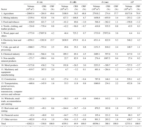
Table 1. Contribution of factors to the changes in total WF.
E(1t) E(1B) E(1m) 1T
Volume CRS CRF Volume CRS CRF Volume CRS CRF Volume CRF
Sector (106m3) (%) (%) (106m3) (%) (%) (106m3) (%) (%) (106m3) (%) 1. Agriculture −20845.4 −204.9 49.6 3100.9 30.5 48.8 27918.2 274.4 57.7 10173.8 79.9
2. Mining industry −2339.4 923.8 5.6 427.3 −168.8 6.7 1658.8 −655.0 3.4 −253.2 −2.0
3. Food and tobacco −636.0 421.7 1.5 −61.2 40.6 −1.0 546.4 −362.2 1.1 −150.8 −1.2
4. Textile, clothing, and leather products
−324.8 −739.4 0.8 −42.2 −96.0 −0.7 410.8 935.5 0.8 43.9 0.3
5. Wood, paper and others
−1773.0 −27697.8 4.2 46.4 725.2 0.7 1733.0 27072.6 3.6 6.4 0.1
6. Electricity, heat and water
−6594.1 −1202.8 15.7 2630.9 479.9 41.4 4511.4 822.9 9.3 548.2 4.3
7. Coke, gas and oil processing
−1060.3 −753.4 2.5 49.6 35.2 0.8 1151.5 818.2 2.4 140.7 1.1
8. Chemical industry −2361.4 −566.4 5.6 289.3 69.4 4.5 2489.1 597.0 5.1 417.0 3.3
9. Non-metallic mineral products
−271.7 −990.4 0.6 22.7 82.9 0.4 276.4 1007.5 0.6 27.4 0.2
10. Metal products −3173.8 436.2 7.6 192.8 −26.5 3.0 2253.5 −309.7 4.7 −727.5 −5.7
11. Machinery and equipment manufacturing
−819.7 387.5 2.0 6.7 −3.2 0.1 601.4 −284.4 1.2 −211.5 −1.7
12. Construction −221.4 −41.1 0.5 −27.4 −5.1 −0.4 787.8 146.1 1.6 539.1 4.2
13. Transportation, postal services, information
transmission, computer services and software
−660.6 −145.9 1.6 53.3 11.8 0.8 1060.0 234.1 2.2 452.8 3.6
14. Wholesale, retail trade, accommodation and catering
−263.7 −36.3 0.6 −50.3 −6.9 −0.8 1040.4 143.2 2.1 726.5 5.7
15. Real estate and renting
−232.5 −49.1 0.6 −164.4 −34.7 −2.6 870.5 183.8 1.8 473.5 3.7
16. Financial sector −42.4 −48.0 0.1 −64.7 −73.2 −1.0 195.4 221.2 0.4 88.3 0.7
17. Other services −402.0 −91.6 1.0 −50.6 −11.5 −0.8 891.3 203.2 1.8 438.7 3.4
Total −42022.1 −330.0 100.0 6359.1 49.9 100.0 48396.1 380.1 100.0 12733.1 100.0
Note: the Total is the sum for each column. The columns for Volume show the volume (106m3)ofE(1t),E(1B),E(1m), and1Tin each sector. Volumes are computed from Eqs. (13), (14), and (15).
The columns of CRS (contribution rate to sector) show the proportion ofE(1t),E(1B), andE(1m) in1Tin each sector. CRS=Volume/(1T)×100 %. The columns of CRF (contribution rate in factor) show the proportion of each sector’sE(1t),E(1B),E(1m), and1Tin the totalE(1t), totalE(1B), totalE(1m), and total1T. CRF=(Volume/Total Volume)×100 %. For example, in the sector of agriculture, the volume ofE(1t) is−2.1×10¹⁰m3; the proportion of thisE(1t) in the1Tin agriculture (1.0×10¹⁰m3)is−204.9 %; the proportion of thisE(1t) in the totalE(1t) (−4.2×10¹⁰m3)is
49.6%.
Table 1. The total WF of the HRB surged from 4.3×10¹⁰m3 (70.9 % of which is IWF) in 2002 to 5.6×10¹⁰m3(65.6 % of which is IWF) in 2007, increasing about 30 %. In fact, the total available water resources (including water transferred from other regions) in the HRB was 4.0×10¹⁰m3 in 2002 and 3.8×10¹⁰m3in 2007 (Haihe River Water Conservancy Commission, 2003, 2008), and this gap between WF and available water resources conforms to the water resources tension in the HRB. The surge in WF is attributable to soar-ing agricultural demand (1.0×10¹⁰m3), and the steady in-crease of WFs for service-related sectors. In the total WF increase of 1.3×10¹⁰m3from 2002 to 2007, 6.1×10⁹m3
29 external water footprint
internal water footprint
0 10 20 30 200 300 400 500 600
1 2 3 4 5 6 7 8 9 10 11 12 13 14 15 16 17 Total
W
at
er
f
oo
tp
ri
nt
(
U
ni
t:
1
0
8 m 3)
2002
Sectors
(a)
external water footprint internal water footprint
0 10 20 30 40 200 300 400 500 600
Sectors
W
at
er
f
oo
tp
ri
nt
(
U
ni
t:
1
0
8 m 3)
2007
1 2 3 4 5 6 7 8 9 10 11 12 13 14 15 16 17 Total
[image:6.595.51.287.57.489.2](b)
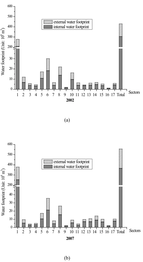
Figure 2. WFs in the HRB in 2002 (a) and 2007 (b) Fig. 2. WFs in the HRB in 2002 (a) and 2007 (b).
Agriculture; electricity, heat, and water; chemical industry; and wood, paper and others had the largest total WFs in both 2002 and 2007. These four WFs account for over 80 % of the total.
As explained above, IWF relates to the use of local water resources in the HRB, and EWF represents the VW in prod-ucts imported from outside and consumed in the HRB. The two kinds of WFs have different effects on water scarcity in a river basin: the IWF consumes local water resources in the river basin, while the EWF is a supplement to save the local water resource, match the demand of products and relieve the pressure on local water resources (Zhang et al., 2012).
From 2002 to 2007, the proportion of EWF in the HRB rose from 29.1 to 34.4 %. Of the 13 sectors with incremental total WFs, the increases in EWFs in 7 sectors are much larger
than their increases in IWFs. This probably relates to gov-ernment policy orientation. Since the 2000s, govgov-ernments in the Haihe River basin have strengthened restrictions on water use in industries. Many water-intensive factories, especially those with large WFs, were forced to improve their water-use efficiency or move out of the basin. In the meantime, high-tech industries with low water intensity and high added value were strongly encouraged.
The agriculture sector experienced the largest expansions in IWF and EWF. As the most water-intensive sector, agri-culture is always the core of Chinese strategies with re-spect to water scarcity. From 2002 to 2007, the agricul-tural IWF in the HRB grew 22.5 %, while the EWF grew 79.1 %, which shows a shift to greater dependence on exter-nal water resources.
In most other sectors, the WFs increased slightly. Of the 13 sectors whose WF increased, 10 sectors’ EWFs had higher growth rates than their IWF; but in electricity, heat and wa-ter; construction; transportation, postal services, information transmission, computer services, and software; wholesale, retail trade, accommodation, and catering; and real estate and renting, the IWF growth rate was close to that of the EWF growth rate. In the financial sector and in other services, the IWF growth was higher than that of the EWF. This is mainly due to the population explosion and development of tertiary industries. As the Chinese political, economic and cultural center, the HRB has advantages in attracting capital and tal-ent that lead to the expansion of the economy and population. Although electricity, heat and water; construction; and the service sectors (no. 13 to no. 17 in Table 1) have relatively low direct and total water coefficients, the huge demands for energy, housing, and services make very large total WFs. Not only the EWFs but also the IWFs in these sectors increased, because some fresh water must be consumed on site rather than be replaced by external VW.
Overall, the WF in the HRB has increased about 30 % and begun to depend more on the EWF while the IWF has begun to be controlled. The sectors with high direct water coeffi-cient and large WF have been the major focus of the basin’s water resources management (Haihe River Water Conser-vancy Commission, 2011). Under the government’s green development strategy, industrial restructuring will continue to play a significant role in water resources conservation in the HRB in the future (Beijing Government, 2010).
3.2 Factors in WF changes
The contributions of the technological effect E(1t),
eco-nomic structural effect E(1B), and scale effectE(1m) to changes in WF in the HRB are shown in Table 1. Positive values indicate an increase in WF, while negative values in-dicate a decrease.
all sectors had significant decreases. In terms of volume changes, theE(1t) for agriculture (−2.1×10¹⁰m3); elec-tricity, heat, and water (−6.6×10⁹m3); and metal products (−3.2×10⁹m3)decreased most, equaling 49.6, 15.7, and 7.6 % of the total E(1t). E(1t) made different
contribu-tions to the changes in WF in different sectors. E(1t) in
the sector of wood, paper, and others had the greatest pro-portional contribution to water conservation (27 697.8 %), whileE(1t) in the sector of wholesale, retail trade,
accom-modation, and catering had the least proportional contribu-tion (36.3 %). For agriculture, irrigacontribu-tion techniques have im-proved to reduce water losses and increase water use effi-ciency. Moreover, water-saving agronomic technologies, for instance, deep plowing, water and soil conservation, and planting drought-resistant varieties, have been widely pop-ularized by the government and enterprises (Beijing Govern-ment, 2010). For manufacturing industries, a set of water-saving mechanisms has been built, characterized by water recycling, reuse, and control (Haihe River Water Conser-vancy Commission, 2011). The volume of industrial water use per value added plummeted from 9.8×10⁻⁵m3RMB−1 to 1.9×10⁻⁵m3RMB−1from 2002 to 2007, which is now much less than that in other regions of China (Beijing Government, 2010).
The scale effect (E(1m), 4.8×10¹⁰m3) was the main contributor to the WF increase, equaling 380.1 % of the final
1T.E(1m) in all 17 sectors grew; the top 3 were agriculture (2.8×10¹⁰m3); electricity, heat, and water (4.5×10⁹m3); and the chemical industry (2.5×10⁹m3), respectively equal-ing 57.7, 9.3, and 5.1 % of the total change in E(1m).
E(1m) made different proportional contributions to the WF changes in different sectors. The increases inE(1m) make up more than 100 % of the total changes, especially in the sectors of wood, paper, and others (27 072.6 %); non-metallic mineral products (1007.5 %); and textile, clothing, and leather products (935.5 %). The increased contribution ofE(1m) was mainly related to population growth and dras-tic demand expansion. From 2002 to 2007, the population of the HRB increased at the rate of 9.2 ‰ per year, much higher than the national average rate of 4.8 ‰ per year, and the scale of final demand soared from 2.4×10¹²RMB year−1 to 6.7×10¹²RMB year−1(Beijing Statistics Bureau, 2003, 2008; Tianjin Statistics Bureau, 2003, 2008; Hebei Statis-tics Bureau, 2003, 2008; National Bureau of StatisStatis-tics, 2003, 2008), which made the contribution of scale effect to the total WF increase. Because population and living standards keep increasing (National Bureau of Statistics, 2008; Haihe River Water Conservancy Commission, 2011), the scale effect may put more pressure on water resources in the future.
The impact of the economic structural effectE(1B) is less
than that of the technological effect and scale effect (49.9 % of the final change), but the absolute amount of E(1B) is
still considerable (6.4×10⁹m3). There were increases in
the E(1B) in 10 sectors. The top three were agriculture
(3.2×10⁹m3); electricity, heat, and water (2.6×10⁹m3);
and the mining industry (4.3×10⁸m3), respectively equal-ing 48.8, 41.4, and 6.7 % of the total change in E(1B).
TheE(1B) of the other seven sectors declined; the biggest
declines were in real estate and renting (−1.6×10⁸m3), the financial sector (−6.4×10⁷m3), and food and tobacco (−6.1×10⁷m3), equaling −2.6, −1.0, and −1.0 % of the total change in E(1B). E(1B) made different
contribu-tions to the WF changes in different sectors.E(1B) in the
sectors of wood, paper, and others (725.2 %); electricity, heat, and water (479.9 %); and non-metallic mineral prod-ucts (82.9 %) made greater proportional contributions to the WF increase than E(1B) in other sectors; and E(1B) in
textile, clothing, and leather products (−96.0 %); the finan-cial sector (−73.2 %); and real estate and renting (−34.7 %) made greater proportional contributions to decreasing their WFs. The economic structural effect, which includes the pro-portion of sectors, demand pattern change, price leverage, change of intermediate products, and economized material input caused by management improvement, reflects the im-pact of industrial restructuring (Chen and Yang, 2011). From 2002 to 2007, the proportion of the agriculture WF in the total WF grew slightly from 64.5 to 68.0 %, while that of services increased from 6.9 to 10.2 %, and that of the man-ufacturing industry declined from 28.6 to 21.8 %. This may relate to the Beijing Olympic Games in 2008, for which the government made a series of industrial restructurings in the HRB. To decrease the WF, industrial restructuring to cre-ate more efficient wcre-ater savings should be undertaken by the government and companies.
We do not analyze the above factors’ contributions to IWF and EWF independently, because they are equivalent to their contributions to the total WF. This is according to the demand-driven view of VW developed by Renault (2003), who noted that the value of VW imported by a region (i.e., EWF) is the volume that the region would have consumed if it had to produce the product itself. Therefore, the EWF could be seen as a replacement that saves IWF and should be treated the same as IWF (Renault, 2003); and thus the factors have the same proportion of effects on them.
4 Discussion
4.1 Implications for water management
The changes in the IWF and EWF of the HRB and the de-composition of the contribution of each factor could be use-ful for evaluating the achievements of past management and policies and for supporting future work on solving the water problems in the HRB.
and tobacco, textiles, and some service sectors. In the fu-ture, industrial restructuring should play a more important role in reducing the pressure on water resources in the HRB or shifting the pressure to the EWF. The agricultural sector remains one of the focal areas. However, shifting to rain-fed farming and/or reducing the size of the agricultural sec-tor may have painful repercussions with respect to prof-its and ecosystems (Zhang et al., 2012). The government should consider protecting the profits of farmers or ensuring proper compensation.
The technological effect is the major factor in offsetting the increase in WF and there are still possibilities for further improvement, which deserve more attention of the govern-ment and enterprises. The marked contribution of the scale effect to the WF increase is mainly attributable to the expan-sion of population and per-capita demand, which indicates that basin planners should consider the capacity of water re-sources in future planning. Importing VW can be a water supplement to mitigate water pressures in the HRB, but con-trolling the growth of the internal water footprint might be more necessary to sustainability in the long term.
The expansion of the EWF shifts the pressure of water de-mand in the HRB to other regions. However, a detailed inves-tigation of the trade-offs of this shift and the VW situation in other regions should be made to evaluate whether this shift makes new water problems in other regions or basins. For example, the increased agricultural scale in southern China seems to have made less increase in its WF than that in west-ern China, which is likely because the former area has much greater precipitation than the latter. Therefore, the former re-gion may be more suitable for exporting VW contained in agricultural products to the HRB.
4.2 Method improvements in the future
The GRIT method introduced in this study is a highly flexible method of processing IO tables that focuses on describing the IO status in a region accurately at the macro level rather than the micro level (Jensen et al., 1979). It has better applicability and accuracy than other methods, such as the biproportional scaling method (Stone, 1961) and Kuroda’s method (1988), when data are lacking. If detailed data on the economic ex-changes between administrative regions are available, the ac-curacy of these other methods will be near to or better than that of the GRIT method, and researchers could choose other methods or combine the GRIT method with them to achieve better accuracy.
The IO method assumes that imports are produced under the same conditions as domestic products (Leontief, 1941; Zhao et al., 2009). This is in accordance with the demand-driven vision of VW, which notes that the value of VW imported by a region is the volume that the region would have consumed if it had to produce the product itself (Re-nault, 2003). In fact, different regions usually have different production situations and the water coefficient vectors are
different. If it is necessary to get the real WF of imported products, the EWFs should be assessed from the perspective of the producing area, which requires a VW and IO analysis for those areas, or even building a multi-regional VW statis-tics system to evaluate the WF of the products in regional trade.
The GRIT-IO-WAD framework for WF could be imple-mented in other river basins. Although the computation of this framework for WF is straightforward, it has similar drawbacks to the IO method. The data requirements are enor-mous because the input and output of each production pro-cess and economic activity circulation propro-cess have to be accounted for, so the IO table is necessary (Leontief, 1941; Zhao et al., 2010). In this study, because of the lack of more detailed data, we used the available IO data for 2002 and 2007 and aggregated the economic sectors into 17 main sec-tors; some aggregation errors are inevitable. A separate anal-ysis of different branches (planting, livestock farming, aqua-culture, and forestry) in agriaqua-culture, which makes up more than half of the total EWF in the HRB, could not be imple-mented. A detailed analysis of WF changes in agriculture and other sectors might be a target for future studies.
5 Conclusions
The input-output (IO) and structural decomposition analy-sis (SDA) models are often used to quantitatively assess the WF changes between different years and the contributions of key economic sectors and factors leading to those changes, called the decomposition analysis of WF changes. However, conventional studies only focus on WF from the tive of administrative regions rather than from the perspec-tive of river basins. In this study, to make a decomposition analysis of WF changes at the river basin scale, we used a framework that combines the generating regional IO ta-bles (GRIT) method, IO, and weighted average decomposi-tion (WAD) method of the SDA model. This GRIT-IO-WAD framework is tested with the example of the Haihe River basin (HRB). Three major factors caused the WF changes, including the technological effect that reflects the contribu-tion of technological changes, the economic structural ef-fect that reflects the contribution of structural relationship changes between sectors, and the scale effect that reflects the contribution of the change in the total amount of final prod-ucts. The following conclusions are reached:
2. The technological effect was the main contributor to counteracting the rise of WF, and it has the poten-tial to reduce the WF by 4.2×10¹⁰m3. The contri-bution of the scale effect played a dominant role in the WF increase, which led to an increase of WF of 4.8×10¹⁰m3. The contribution of the economic struc-tural effect to the WF is relatively less, but led to an increase in WF of 6.4×10⁹m3. Therefore, the gov-ernment and enterprises should keep developing tech-nologies, adjusting the industrial structure to encour-age water-saving methods, and controlling the growth of production.
Acknowledgements. The authors thank the International Science &
Technology Cooperation Program of China (no. 2011DFA72420), the National Science Foundation for Innovative Research Group (no. 51121003), the National Basic Research Program of China (no. 2010CB951104), and the Fundamental Research Funds for the Central Universities for their financial support.
Edited by: Y. Cai
References
Allan, J. A.: Virtual water: a strategic resource. Global solutions to regional deficits, Ground Water, 36, 545–546, 1998.
Allan, J. A.: A convenient solution, The UNESCO Courier, 52, 29– 31, 1999.
Beijing Government: Beijing Green-Development Strategy in Na-tional 12th Five-Year Plan, available at: http://zhengwu.beijing. gov.cn/ghxx/sewgh/t1198652.htm (last access: 9 August 2010), 2010.
Beijing Statistics Bureau: Beijing input-output tables 2002, China Statistics Press, Beijing, 2003.
Beijing Statistics Bureau: Beijing input-output tables 2007, China Statistics Press, Beijing, 2008.
Chen, X. K.: Shanxi water resource input-occupancy-output table and its application in Shanxi Province of China, The 13th Inter-national Conference on Input-output Techniques, Macerata, Italy, 21–25 August 2000, Abstract number 8, 2000.
Chen, X. K. and Yang, C. H.: Input-Output Technique, Science Press, Beijing, 2011.
Chen, Y., Zhang, D. Q., and Savenije, H. H. G.: Water demand man-agement: A case study of the Heihe River Basin in China, Phys. Chem. Earth, 30, 408–419, 2005.
Chen, Z. M. and Chen, G. Q.: Virtual water accounting for the glob-alized world economy: National water footprint and international virtual water trade, Ecol. Indicat., 28, 142–149, 2013.
Dietzenbacher, E. and Los, B.: Structural decomposition technique: Sense and sensitivity, Econ. Syst. Res., 10, 307–323, 1998. Dietzenbacher, E. and Velázquez, E.: Analyzing Andalusian virtual
water trade in an input-output framework, Reg. Stud., 41, 251– 262, 2007.
Feng, K., Siu, Y. L., Guan, D., and Hubacek, K.: Assessing re-gional virtual water flows and water footprints in the Yellow River Basin, China: A consumption based approach, Appl. Ge-ogr., 32, 691–701, 2012.
Guo, C. X.: An analysis of the increase of CO2emission in China – Based on SDA technique, China Industrial Econom., 12, 47–56, 2010.
Haihe River Water Conservancy Commission: Haihe River Year-book 2002, FangZhi Press, Beijing, 2003.
Haihe River Water Conservancy Commission: Haihe River Year-book 2007, FangZhi Press, Beijing, 2008.
Haihe River Water Conservancy Commission: Haihe River Year-book 2010, FangZhi Press, Beijing, 2011.
Hebei Statistics Bureau: Hebei input-output tables 2002, China Statistics Press, Beijing, 2003.
Hebei Statistics Bureau: Hebei input-output tables 2007, China Statistics Press, Beijing, 2008.
Hoekstra, A. Y.: The water footprint of modern consumer society, Routledge, London, 2013.
Hoekstra, A. Y. and Chapagain, A. K.: Water footprints of nations: Water use by people as a function of their consumption pattern, Water Resour. Manag., 21, 35–48, 2007.
Hoekstra, A. Y. and Hung, P. Q.: Virtual water trade: a quantifica-tion of virtual water flows between naquantifica-tions in relaquantifica-tion to interna-tional crop trade. Value of Water Research Report Series No. 11. UNESCO-IHE, Delft, 2002.
Hoekstra, A. Y. and Hung, P. Q.: Globalisation of water resources: International virtual water flows in relation to crop trade, Global Environ. Change, 15, 45–56, 2005.
Hoekstra, R. and van den Bergh, J. C. J. M.: Structural decompo-sition analysis of physical flows in the economy, Environ. Re-source Econ., 23, 357–378, 2002.
Hoekstra, A. Y. and van den Bergh, J. C. J. M.: Comparing structural and index decomposition analysis, Energ Econ., 25, 39–64, 2003. Hoekstra, A. Y., Chapagain, A. K., Aldaya, M. M., and Mekon-non, M. M.: The Water Footprint Assessment Manual: Setting the Global Standard, Earthscan, London, 2011.
Hubacek, K. and Sun, L.: Economic and societal changes in China and their effects on water use: A scenario analysis, J. Ind. Ecol., 9, 187–200, 2005.
Jensen, R. C., Mandeville, T. D., and Karunarate, N. D.: Regional economic planning: generation of regional input-output analysis, Groom Helm, London, 1979.
Kanada, N.: Land resources and international trade, Taga Shuppan, Tokyo, 2001.
Kondo, K.: Economic analysis of water resources in Japan: Using factor decomposition analysis based on input-output tables, Env-iron. Econ. Pol. Stud., 7, 109–129, 2005.
Kuroda, M.: A Method of Estimation for the Updating Transac-tion Matrix in the Input-Output RelaTransac-tionships, in: Statistical Data Bank Systems, edited by: Uno, K. and Shishido, S., North Hol-land, Amsterdam, 213–251, 1988.
Lenzen, M.: Understanding virtual water flows: A multi-region IO case study of Victoria, Water Resour. Res., 45, w09416, doi:10.1029/2008WR007649, 2009.
Leontief, W.: The Structure of the American Economy, Oxford Uni-versity Press, Oxford, 1941.
Li, J. H.: A weighted average decomposition method of SDA model and its application in Chinese tertiary industry development, Syst. Eng., 22, 69–73, 2004.
Mekonnen, M. M. and Hoekstra, A. Y.: The blue water footprint of electricity from hydropower, Hydrol. Earth Syst. Sci., 16, 179– 187, doi:10.5194/hess-16-179-2012, 2012.
Ministry of Water Resources: China Water Resources Bulletin 2002, China Water & Power Press, Beijing, 2003.
Ministry of Water Resources: China Water Resources Bulletin 2007, China Water & Power Press, Beijing, 2008.
National Bureau of Statistics: China Statistical Yearbook 2002, China Statistics Press, Beijing, 2003.
National Bureau of Statistics: China Statistical Yearbook 2007, China Statistics Press, Beijing, 2008.
Renault, D.: Value of Virtual Water in Food: Principles and Virtues, Value of water research report series No.12. UNESCO-IHE, Delft, 2003.
Schendel, E. K., Macdonald, J. R., Schreier, H., and Lavkulich, L. M.: Virtual water: a framework for comparative regional resource assessment, J. Environ. Assess. Pol. Manag., 9, 341–355, 2007. Stone, R.: Input-Output and National Accounts, Organization for
European Economic Cooperation, Paris, 1961.
Tianjin Statistics Bureau: Tianjin input-output tables 2002, China Statistics Press, Beijing, 2003.
Tianjin Statistics Bureau: Tianjin input-output tables 2007, China Statistics Press, Beijing, 2008.
Vanham, D., Mekonnen, M. M., and Hoekstra, A. Y.: The water footprint of the EU for different diets, Ecol. Indicat., 32, 1–8, 2013.
Verma, S., Kampman, D. A., Zaag, P., and Hoekstra, A. Y.: Going against the flow: A critical analysis of inter-state virtual water trade in the context of India’s National River Linking Program, Phys. Chem. Earth, 34, 261–269, 2009.
Wang, Z. Y., Huang, K., Yang, S. S., and Yu, Y. J.: An input-output approach to evaluate the water footprint and virtual water trade of Beijing, China, J. Clean. Prod., 42, 172–179, 2013.
Wheida, E. and Verhoeven, R.: The role of “virtual water” in the water resources management of the Libyan Jamahiriya, Desali-nation, 205, 312–316, 2007.
Yang, H. and Zehnder, A.: “Virtual water”: An unfolding concept in integrated water resources management, Water Resour. Res., 43, W12301, doi:10.1029/2007WR006048, 2007.
Zeng, Z., Liu, J., Koeneman, P. H., Zarate, E., and Hoekstra, A. Y.: Assessing water footprint at river basin level: a case study for the Heihe River Basin in northwest China, Hydrol. Earth Syst. Sci., 16, 2771–2781, doi:10.5194/hess-16-2771-2012, 2012. Zhang, Z. Y., Shi, M. J., Yang, H., and Chapagain, A.: An IO
analy-sis of the trend in virtual water trade and the impact on water re-sources and uses in China, Econ. Syst. Res., 23, 431–446, 2011a. Zhang, Z. Y., Yang, H., and Shi, M. J.: Analyses of water foot-print of Beijing in an interregional input-output framework, Ecol. Econ., 70, 2494–2502, 2011b.
Zhang, Z. Y., Shi, M. J., and Yang, H.: Understanding Beijing’s wa-ter challenge: A decomposition analysis of changes in Beijing’s water footprint between 1997 and 2007, Environ. Sci. Tech., 46, 12373–12380, 2012.
Zhao, J. Z., Liu, W. H., and Deng, H.: The potential role of virtual water in solving water scarcity and food security problems in China, Int. J. Sustain. Dev. World Ecol., 12, 419–428, 2005. Zhao, N. Z. and Samson, E. L.: Estimation of virtual water
con-tained in international trade products using nighttime imagery, Int. J. Appl. Earth Obs., 18, 243–250, 2012.
Zhao, X., Chen, B., and Yang, Z. F.: National water footprint in an IO framework-A case study of China 2002, Ecol. Model., 220, 245–253, 2009.
Appendix A
List of abbreviations
EWF: external water footprint GRIT: Generating regional IO tables HRB: Haihe River basin
IO: input-output
IWF: internal water footprint
SDA: Structural decomposition analysis VW: virtual water