One way coupling of an integrated assessment model and a water resources model: evaluation and implications of future changes over the US Midwest

www.hydrol-earth-syst-sci.net/17/4555/2013/ doi:10.5194/hess-17-4555-2013

© Author(s) 2013. CC Attribution 3.0 License.

Hydrology and

Earth System

Sciences

One-way coupling of an integrated assessment model and a water

resources model: evaluation and implications of future changes over

the US Midwest

N. Voisin1, L. Liu2, M. Hejazi2, T. Tesfa1, H. Li1, M. Huang1, Y. Liu1, and L. R. Leung1

1_{Pacific Northwest National Laboratory, Richland, WA, USA}

2_{Joint Global Change Research Institute, Pacific Northwest National Laboratory, College Park, MD, USA}

Correspondence to: N. Voisin ([email protected])

Received: 2 April 2013 – Published in Hydrol. Earth Syst. Sci. Discuss.: 22 May 2013 Revised: 14 September 2013 – Accepted: 10 October 2013 – Published: 18 November 2013

Abstract. An integrated model is being developed to

ad-vance our understanding of the interactions between human activities, terrestrial system and water cycle, and to evalu-ate how system interactions will be affected by a chang-ing climate at the regional scale. As a first step towards that goal, a global integrated assessment model, which in-cludes a water-demand model driven by socioeconomics at regional and global scales, is coupled in a one-way fashion with a land surface hydrology–routing–water resources man-agement model. To reconcile the scale differences between the models, a spatial and temporal disaggregation approach is developed to downscale the annual regional water demand simulations into a daily time step and subbasin representa-tion. The model demonstrates reasonable ability to repre-sent the historical flow regulation and water supply over the US Midwest (Missouri, Upper Mississippi, and Ohio river basins). Implications for future flow regulation, water sup-ply, and supply deficit are investigated using climate change projections with the B1 and A2 emission scenarios, which affect both natural flow and water demand. Although natu-ral flow is projected to increase under climate change in both the B1 and A2 scenarios, there is larger uncertainty in the changes of the regulated flow. Over the Ohio and Upper Mis-sissippi river basins, changes in flow regulation are driven by the change in natural flow due to the limited storage capac-ity. However, both changes in flow and demand have effects on the Missouri River Basin summer regulated flow. Changes in demand are driven by socioeconomic factors, energy and food demands, global markets and prices with rainfed crop demand handled directly by the land surface modeling

com-ponent. Even though most of the changes in supply deficit (unmet demand) and the actual supply (met demand) are driven primarily by the change in natural flow over the entire region, the integrated framework shows that supply deficit over the Missouri River Basin sees an increasing sensitivity to changes in demand in future periods. It further shows that the supply deficit is six times as sensitive as the actual sup-ply to changes in flow and demand. A spatial analysis of the supply deficit demonstrates vulnerabilities of urban areas lo-cated along mainstream with limited storage.

1 Introduction

processes governing the interactions in the coupled human– earth system are not fully understood.

Global integrated models are being developed (Pokhrel et al., 2012; Biemans et al., 2011; Döll et al., 2009; Hadde-land et al., 2006) to advance our understanding of the in-teractions between human activities, the terrestrial water cy-cle, and how they will be affected by the changing climate at regional and global scales. In those models, water de-mands are represented using physically-based models, usu-ally related to irrigation demands simulated by crop mod-els, while water demands from other sectors such as energy are ignored or prescribed. At regional scales, assessments of climate change impacts on water resources have been per-formed using hydrologic models driven by climate change scenarios, with or without water management and usually as-suming no change in land use (e.g., Backlund et al., 2008). Recently some analyses have been performed combining the effect of land use change and climate change on natural water resources, with land use primarily driven by population and urbanization while changes in agriculture or effects of reser-voir operations are not considered (Cuo et al., 2011; Mishra et al., 2010). Although these studies have provided impor-tant insights on future changes in water resources driven by climate change and/or land use change, with or without adap-tation by water management, none have fully reconciled the socioeconomic, land use, energy, water demand, and climate drivers used to assess the hydrologic impacts and water man-agement options.

This study represents a step towards developing an in-tegrated framework that represents both human and natu-ral system drivers of water cycle and climate changes with the goal towards a fully coupled modeling system that rec-onciles the hydrology and water management simulated at local/regional scales with water demand and land use driven by socioeconomics at regional/global scales. A one-way coupling is presented to first address the scaling chal-lenge and evaluate the skill of the models. We implement a subbasin configuration of a land surface model to sim-ulate available water (runoff and baseflow) coupled with a river routing model (Model for Scale Adaptive River Trans-port or MOSART) and a water resources management model (WM), and a global integrated assessment model (IAM). The adopted IAM simulates water demand by sector (irrigation, domestic, industrial, etc.) driven by socioeconomic factors, technologically detailed energy and food demands, and cli-mate mitigation targets in a fully integrated system. However, the IAM does not yet account for climate change impacts on water demands. The modeling of water demands is focused mainly on the implications of climate mitigation policies, so-cioeconomic drivers (population, income, food and energy demands, etc.), and technological change implications. In this study, thus, climate change impacts are primarily cap-tured through changes in water availability, and consequently in water supply deficits.

The linkage of the Global Change Assessment Model (GCAM) and a subbasin implementation of the Community Land Model (SCLM) facilitates the propagation of human decisions pertaining to water demand per sector and tech-nology from the assessment decision framework to SCLM at the appropriate temporal and spatial scales. Although this coupling is still one way (i.e., no feedback is considered from SCLM-MOSART-WM to GCAM), it constitutes a key step toward establishing a consistent, integrated framework of water modeling that is portable, consistent with global modeling and analyses, and provides significant improve-ments and insights into the interaction of human decisions and climate changes at regional scales. The proposed one-way coupling of an IAM (i.e., GCAM) and an earth system model or ESM (i.e., SCLM) aims at improving the represen-tation of the interaction pathways that govern the evolution of the hydrologic components that are integral to the energy, water and land components of the Earth system, in the con-text of changing climate. By accounting for water demands as a function of the socioeconomic factors, energy and food demands, global markets and prices, IAMs provide an eco-nomic platform to meaningfully represent human activities and their roles in affecting the water cycle.

The paper describes the methodology to couple the water demand component of a global integrated assessment model to the terrestrial system component, consisting of a land sur-face model, a river routing model and a water resources man-agement model of an earth system model (ESM). The in-tegrated models are driven by global simulations of current and future climates and are evaluated over the historical pe-riod using observations. Implications of combined changes in climate and human factors (socioeconomics, energy and food demands, and climate mitigation targets represented by the global integrated assessment model) on future water re-sources are assessed from simulations by the integrated mod-els for future time periods. This study brings global model-ing efforts on climate change impacts and related mitigation activities to the regional scale, with a focus on modeling and analysis over the US Midwest with strong interactions among water, energy, and land use.

The next section presents the domain and the models. Sec-tion 3 describes the approach to couple the demand model to the terrestrial system model. Section 4 evaluates the inte-grated model over the historical period, assesses implications for the future and identifies the drivers of change.

2 Domain, models and datasets

2.1 Domain

The US Midwest region is chosen for the first application of the integrated models. The domain includes the Missouri, Upper Mississippi and Ohio River basins (Fig. 1), hereinafter denoted as the Midwest Region. The crop in the region is

56 2

3

Figure 1: GRanD reservoir database by type of operating rules over the three regions of the Midwest: Missouri, Upper

4

Mississippi and Ohio. Flow is validated at the outlet of the three regions: Missouri at Hermann (06934500), Upper

5

Mississippi at Grafton (05587450) and Ohio at Metropolis (03611500).

6 7

Fig. 1. GRanD reservoir database by type of operating rules over the three regions of the US Midwest targeted in this study: Missouri, Upper Mississippi and Ohio. Flow is validated at the outlet of the three regions: Missouri at Hermann (06934500), Upper Mississippi at Grafton (05587450) and Ohio at Metropolis (03611500).

mostly rainfed over the Upper Mississippi, Ohio and North-ern Missouri river basins. Natural flow has been shown, at least over the Upper Mississippi river basin (Frans et al., 2013; Mishra et al., 2010), to be more sensitive to climate change than to land use change. However, this region repre-sents many crosscutting issues on climate, energy, land use, and water, including water quality. For example, the US Mid-west is a major area for bioenergy resource, representing po-tential conflicts between food and fuel. In addition, the US Midwest is of primary importance for regional and interna-tional water markets, and hence represents an interesting test case for our modeling framework that aims to model global water transfer in the future.

There are 476 geo-referenced reservoirs over the region (GRanD database, Lehner et al., 2008) and all of them are modeled in the study (Fig. 1). Despite their small capaci-ties, Lehner et al. (2011) demonstrated their importance in the regulation of the flow at larger scales. Also, keeping all reservoirs in the model allows us to test the model for poten-tial applications across multiple spapoten-tial scales in the future.

The Missouri River has its headwater in the Rockies, which provides a late spring water storage for the agricul-ture rich region. The Missouri River Basin has 194 reservoirs according to the GRanD database (Lehner et al., 2008); out of those reservoirs, 125 are used for irrigation and not flood control, 29 are used jointly for both irrigation and flood con-trol, and the remaining 40 reservoirs are used for other uses like hydropower and supply (Fig. 1). The Upper Missouri is used mostly for combined flood control and irrigation, the Platte River and the upper Kansas River are used for irriga-tion but not flood control, while the downstream Kansas and Osage rivers are used mostly for flood control and not

irriga-tion. The most downstream station along the Missouri River before its confluence with the Mississippi River is Hermann, MO, which drains 1 371 010 km2of semi-arid lands.

The Ohio River Basin lies in the eastern part of the do-main with its headwater in the Appalachians and is the do-main tributary in volume to the Mississippi River (Fig. 1). The Ohio River basin has 131 reservoirs according to the GRanD database; none are used for irrigation, 71 are used in part for flood control. Other usages include navigation, recreation, hydropower or water supply as this is a heavily populated region (25 million, 8 % of the US population; Ohio River Valley Sanitation Commission). The downstream station is Metropolis, IL, which drains 525 727 km2of humid subtrop-ical and humid continental climate areas.

The Upper Mississippi River has its headwaters above Minneapolis. The basin includes 220 reservoirs with none for irrigation and 25 for flood control. Above Minneapolis, reser-voirs are mostly for hydropower and recreation while down-stream reservoirs are mostly for navigation; 112 of them have a reservoir capacity of less than 500 million cubic meters. The downstream station prior to the confluence with the Mis-souri is Grafton, IL (443 475 km2).

Reservoir regulation for navigation is a priority in the Ohio River basin, the Upper Mississippi River basin, and along the main stem of the Missouri River. In our generic water re-sources model detailed below, operating rules differ for (i) irrigation only, (ii) combined irrigation and flood control, and (iii) other usages. The operating rule for other usages is consistent with navigation, with the aim to have a uniform flow throughout the year. However, over the main stem of the Missouri River the priority is given to irrigation, which pre-scribes seasonality in the monthly releases. Control for navi-gation requires joint operations between reservoirs of differ-ent storage capacity, with coordination for withdrawals over multiple timescales, which are not represented here. How-ever, at a monthly timescale, the effect of reservoir regulation on streamflow matches reasonably well the observed regu-lated flow, as shown in Voisin et al. (2013) and in the next sections.

2.2 Models and datasets

57 1

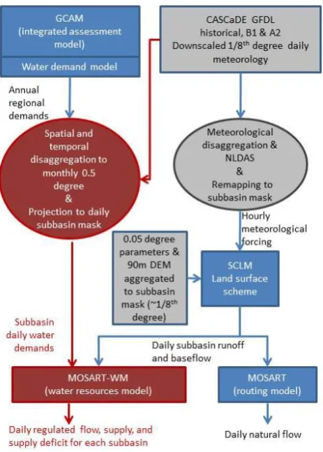
Figure 2: Schematic of the system. The paper describes and evaluates the coupling of the water demand model with the

2

water resources model (red). Publicly available datasets processed for the experiments are in grey. Models are in blue.

3 Fig. 2. Schematic of the system. The paper describes and evaluates

the coupling of the water demand model with the water resources model (red). Publicly available datasets processed for the experi-ments are in grey. Models are in blue.

statistically downscaled from global climate model simula-tions for the historical and future periods (Fig. 2). The next sections present details about the different models.

2.2.1 A subbasin-based framework for land surface

hydrologic modeling

In this study, we applied the subbasin-based version of Com-munity Land Model version 4 (hereinafter denoted as SCLM, Li et al., 2013b; Tesfa et al., 2013), for hydrologic sim-ulations over the study region. CLM is the land compo-nent within the Community Earth System Model (CESM) (formerly known as Community Climate System Model) (CCSM) (Lawrence et al., 2011). CLM is also the land sur-face component in a regional earth system model based on the Weather Research and Forecasting (WRF) model (Ke et al., 2012; Kraucunas et al., 2013; Leung et al., 2006). The capability of CLM4 for hydrologic simulations has re-cently been assessed at small watershed to larger basin scales (Huang et al., 2013; Li et al., 2011, 2013b; Tesfa et al., 2013). CLM simulates the full energy and water balances for a mosaic of rainfed vegetation classes, including crop.

CLM provides the runoff and baseflow for the water man-agement model. In the subbasin-based framework, land sur-face hydrologic processes such as water and energy trans-fers between the land surface and the atmosphere, as well runoff generation, are represented by treating each subbasin as a pseudo-grid cell without significantly modifying the ex-isting CLM modeling structure. Subbasin boundaries within the study domain were delineated using ArcSWAT (Neitsch et al., 2005). The study area was delineated into 18 681 sub-basins with∼120 km2average size, equivalent to 1/8th de-gree grid cells, making it comparable to the North Ameri-can Land Data Assimilation System (NLDAS2) (Cosgrove et al., 2003). Soil, vegetation and land cover characteris-tics of each subbasin (∼1/8th degree) in the study domain were derived from the high resolution 0.05◦ CLM4 input dataset developed by Ke et al. (2012), by overlaying the wa-tershed boundaries with the data layers and aggregating to each basin using an area weighted average algorithm, fol-lowing Li et al. (2013b). Hydrologic parameters relevant to topography were obtained by processing the 90 m resolution DEMs from HydroSHEDS (Lehner et al., 2008), consistent with the SCLM model setup in Li et al. (2011, 2013b), Huang et al. (2013) and Tesfa et al. (2013). SCLM was spun up us-ing hourly forcus-ing described below for the historical period 1976–1999 for 10 cycles (300 yr total), until all the state vari-ables reached equilibrium.

2.2.2 Atmospheric forcing data

Daily precipitation and temperature at 1/8th degree resolu-tion were retrieved from the Computaresolu-tional Assessments of Scenarios of Change for the Delta Ecosystem (CASCaDE) dataset (http://cascade.wr.usgs.gov). The CASCaDE dataset was developed by applying the constructed analog statistical downscaling method (Hidalgo et al., 2008) to the historical and future climate simulations generated by the Geophysical Fluid Dynamics Laboratory Coupled Climate Model (GFDL CM2.1) (Delworth et al., 2006) for the Coupled Model In-tercomparison Project (CMIP3). The future climate simula-tions follow the Special Report for Emission Scenarios SRES B1 and A2 emission scenarios. The 1/8th degree downscaled daily precipitation and temperature time series from 1975– 2100 were further processed with the forcing disaggregator of the Variable Infiltration Capacity model (VIC) (Liang et al., 1994) (www.hydro.washington.edu/Lettenmaier/Models/ VIC/Documentation/VICDisagg.shtml) to generate hourly precipitation, temperature, and shortwave radiative fluxes us-ing the MTCLIM 4.2 algorithm (Thornton and Runnus-ing, 1999; Thornton et al., 2000); incoming longwave radia-tion fluxes (the Tennessee Valley Authority algorithm, TVA, 1972); and specific humidity (Kimball et al., 1997) re-quired by SCLM. Wind speed and surface pressure data were obtained from the North American Land Data Assim-ilation System (NLDAS) (Mitchell et al., 2004). The hourly 1/8th degree meteorological data were then projected to the

subbasin boundaries discussed earlier using an area average algorithm as input into SCLM (Fig. 2). The GFDL-B1 and GFDL-A2 scenarios portray the B1 and A2 emissions scenar-ios (optimistic and pessimistic, respectively) as modeled by the GFDL CM2.1 model, which has climate sensitivity in the medium range among the IPCC AR4 models. The B1 emis-sion scenario corresponds to the lowest increase in surface temperature among the different greenhouse gas emission scenarios. Economically, it focuses on global environmen-tal sustainability. The A2 scenario concentrates on regional economic development and is one of the scenarios with the largest temperature increase (IPCC, 2007). Although the at-mospheric forcings used in SCLM-MOSART-WM are con-sistent with the climate scenarios in GCAM with regard to the total radiative forcings, GCAM does not explicitly use any gridded climate data as input. The CASCaDE data are simply used to guide the temporal downscaling in a post-processing step of the GCAM simulated water demand from annual to daily scale, as will be discussed in Sect. 3.2 (Fig. 2).

2.2.3 The water resources management model

(MOSART-WM)

The water resources model (WM, Voisin et al., 2013) re-lies on generic operating rules adjusted independently for each reservoir; monthly release targets are based on the long-term mean monthly inflow, the long-long-term mean monthly de-mand associated to each reservoir, and reservoir characteris-tics (storage and uses). Initial work by Hanasaki et al. (2006) and Biemans et al. (2011) included two types of rules in par-ticular: (i) monthly varying releases based on water demand, hydroclimatic characteristics and storage capacity for reser-voirs used for irrigation, or (ii) for all other uses release of mean annual flow adjusted for monthly demand anomalies (flood control, navigation, conservation, recreation). Voisin et al. (2013) updated the release targets and complemented them with storage targets in order to improve joint flood con-trol and irrigation uses. The WM includes (i) a local extrac-tion module that extracts from the local surface water and river channel to provide in priority for the local demand; (ii) a reservoir module that simulates the reservoir storage, regulates the releases and provides supply to each grid cell in need; and (iii) an interdependency database that assigns to each reservoir a list of subbasins that can receive water from that reservoir and controls the weighted distribution of the supply, and similarly assigns to each subbasin the list of reservoirs it can request water from and controls the weighted distribution of the demand to each reservoir (see Voisin et al., 2013 for further details). The seasonal patterns of the oper-ating rules is monthly, and there is interannual variability of those monthly preset releases based on the initial storage at the start of the irrigation season. However, the extraction is performed at the time step of the run – presently daily. Re-leases adjustment for spilling, minimum environmental flow and drying reservoirs are also made at the time step of the

run. The WM is coupled to the Model for Scale Adaptive River Routing (MOSART) (Li et al., 2013a) river routing model. In this experiment, MOSART-WM is run indepen-dently of the land surface model (SCLM) described above. The return flow is, however, implicitly simulated as we only extract the GCAM consumptive use rather than the with-drawals. The dynamic coupling is an area of research and in particular we investigate the effect that the uncertainties in the localization of the extraction and the redistribution of water will have on the overall modeling. Input for MOSART-WM includes daily surface and subsurface runoff, and daily total water consumptive demand, not withdrawals, provided by the water demand model described below. However, an estimate of withdrawals is used for the optimal calibration of the release targets, as explained in Voisin et al. (2013).

2.2.4 GCAM

The global change assessment model (GCAM) is a dynamic-recursive model that encompasses technologically-detailed representations of human and natural systems and their in-teractions (Wise et al., 2009; Kim et al., 2006; Clarke et al., 2007a, b; Brenkert et al., 2003). The model includes repre-sentations of the global economy, the energy system, agricul-ture and land use, and climate. It models global trade in fossil energy and agricultural products and solves for prices of all energy, agricultural, and forest productivities to balance off demands and supplies (Calvin et al., 2013). This is useful, even though the focus of the work is regional in nature (e.g., US Midwest), because global decisions associated with ad-hering to the adopted B1 and A2 climate mitigation scenarios have regional implications (e.g., bioenergy production in the Midwest Region).

58 1

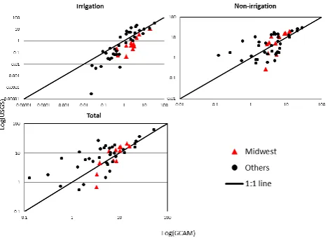
Figure 3: Comparison of GCAM water withdrawal values in year 2005 to USGS values (log-log scale) by states of the

2

United States, and for the Midwestern states.

3 4

Fig. 3. Comparison of GCAM water withdrawal values in year 2005 to USGS values (log-log scale) by states of the United States, and for the Midwestern states.

mention the modeling uncertainties and scale differences be-tween GCAM and SCLM, the suggested demand by GCAM might end up being infeasible when integrated with SCLM-MOSART-WM. In this research, we track the amount of sup-ply deficit (i.e., unmet consumptive water demands) to pro-vide insights on requirements for future implementation of a two-way coupled framework in which unmet consumptive water demands determined by SCLM-MOSART-WM will be used to constrain the GCAM water demand. More de-tails about the water demand methodology in GCAM can be found in Hejazi et al., 2013a).

3 Coupling of the water demand and water

management models

A one-way coupling between GCAM and SCLM-MOSART-WM is the focus of this paper, where GCAM provides the water demand and SCLM-MOSART-WM computes the wa-ter availability and estimates the actual wawa-ter supply. There is, however, a mismatch in scale both spatially and tempo-rally among the models. GCAM is solved on a 5 yr time step and operates at the regional scale (14 geopolitical regions and 151 agro-ecological zones (AEZs)), which are much coarser than what is required by SCLM-MOSART-WM. The tempo-ral and spatial disaggregations to the subbasin mask and daily resolution of MOSART-WM need to represent spatiotempo-ral variations of use over the basin. This has implications for the locally available water supply and affects the WM as operating rules of each reservoir are a function of the monthly climatology and magnitude of the demand associ-ated to each reservoir. Disaggregation affects the distribution of water supply to the different subbasins. Thus, to facilitate the proposed coupling, both spatial and temporal downscal-ing steps were employed, as described next. Note that due

Table 1. Correlation coefficients between GCAM and USGS based on state-level water demand estimates by sector; correlation values in parenthesis are based on the Miwestern states only.

Water demand 1990 2005

sectors Consumption Withdrawal Withdrawal∗

Irrigation 0.86 (0.80) 0.75 (0.91) 0.77 (0.99) Non-irrigation 0.78 (0.77) 0.58 (0.93) 0.80 (0.87)

Total 0.84 (0.80) 0.77 (0.57) 0.87 (0.87)

∗_{USGS does not provide consumptive water use data for 2005.}

to the lack of available tools to downscale land use from the 151-AEZ scale in GCAM to the grid/subbasin scale, SCLM-MOSART-WM presently uses the same land use in the future conditions as defined by the current conditions. Reconcilia-tion of land use between the global and regional models is an ongoing research focus for future improvement of the mod-eling framework.

3.1 Spatial downscaling

We adopted the downscaling methodology of Hejazi et al. (2013b) to downscale the individual sectoral demands (irrigation, livestock, municipal, electricity generation, pri-mary energy, and manufacturing water demands) from re-gional scale (AEZ and GCAM rere-gional scale) to the grid scale (0.5◦×0.5◦), and subsequently to the subbasin scale (Fig. 2). In a nutshell, the downscaling algorithms employ proxy information such as population and areas equipped with irrigation information to map water demands to a finer spatial scale of 0.5◦_{. To assess the accuracy of GCAM in}

combination with the downscaling algorithms in estimating water demands at the regional scale, the spatially downscaled annual sectoral water demands from GCAM are compared against the state-level USGS inventory for the years 1990 and 2005. The six sectors of water demand are sorted into irriga-tion and non-irrigairriga-tion (electricity+domestic+mining+ livestock+manufacturing) water demands for the purpose of simplification. The total water withdrawals and consump-tive use produced by GCAM show a good agreement with USGS values on the state level (Fig. 3). The statistics of the results are shown in Table 1.

3.2 Temporal downscaling

GCAM estimates annual demands every five years (GCAM is run with a 5 yr time interval), which need to be tempo-rally disaggregated to daily scale for input into MOSART-WM. The temporal downscaling is performed independently for each water use sector in several steps: first a continu-ous annual time series of water demands is obtained by lin-early interpolating between the 5 yr intervals. Then the an-nual values are downscaled to monthly through a suite of

techniques as described below; and, finally, the monthly de-mands are downscaled to daily using a uniform distribution. This section presents the disaggregation to the monthly timescale. Wada et al. (2011) devised a set of simple methods to map non-irrigation sectors from annual to monthly time step. We adopted their approaches for domestic, mining, live-stock and manufacturing, extended the electricity generation technique, and simplified the irrigation one. Each of the steps is described next with validation results.

3.2.1 Irrigation

Unlike the work of Wada et al. (2011) who used a crop growth model to estimate monthly irrigation water require-ments, crop water requirements in GCAM are computed us-ing a simplified methodology that utilizes estimated coef-ficients of water requirement per crop type and AEZ from crop growth models to efficiently compute irrigation water on an annual basis (see Chaturvedi et al., 2013). This re-duced form is essential to the computational feasibility of iterating food demands and prices hundreds of iterations in each GCAM time period without resorting to running a crop growth model that many times. Also, adopting the use of a gridded physically-based crop growth model would require downscaling the evolution of land use (e.g., cropland expan-sion) in GCAM for future time periods, a capability that is not yet available and requires future research. GCAM esti-mates annual irrigation demands every five years (GCAM is run with a 5 yr time interval). Chaturvedi et al. (2013) pro-vide a detailed comparison to the other literature estimates and statistics on irrigation estimates at the regional scale; see Chaturvedi et al. (2013), Hejazi et al. (2013a, b) for further details. Figure 3 shows a comparison of the estimated total ir-rigation against USGS estimates for water withdrawals at the state level in year 2005. The next step is to temporally down-scale GCAM results of irrigation water demand to monthly time series.

The monthly profile for downscaling GCAM irrigation water demand from annual to monthly was obtained from Siebert and Döll (2008) by using irrigation results from the Global Crop Water Model (GCWM). GCWM provided global gridded monthly irrigation water requirements for 26 crop types, which were mapped to the twelve GCAM crop categories to estimate the crop and region specific monthly distribution of irrigation. This enabled us to construct irri-gation water use monthly profiles for each of the AEZ re-gions in the US (Fig. 4a). Following the work of Hanasaki et al. (2013a, b), we applied the same monthly profile for irri-gation water withdrawal and consumption. Therefore, irriga-tion water withdrawal and consumpirriga-tion from GCAM were downscaled from annual to monthly time step by applying the ratios calculated from the monthly profiles distinguished by AEZ (Eq. 1).

Wij=Wj×RatioAEZij (1)

whereWiindicates irrigation water demand for the month of

iin yearj, andWj indicates annual irrigation water demand.

3.2.2 Electricity

In this study, the temporal downscaling of electricity gen-erating water demands in the US was built on the basis of electricity use fluctuations within a year. We assume that the amount of water used for generating electricity in a particular month is proportional to the amount of electricity generated in each month. In GCAM, electricity generation is consumed by three main sectors: industry, transportation, and building. Industry and transportation sectors are assumed to consume equal shares of electricity within a year (i.e., uniform dis-tributions). A simple algorithm is developed to reflect the seasonal fluctuations of electricity use in the building sec-tor based on the concepts of heating degree days (HDD) and cooling degree days (CDD). HDD and CDD are measure-ments designed to reflect the demand for energy needed to heat/cool a building. It is derived from measurements of out-side air temperature.

About 20 % of the total electricity used in buildings in the US is used for heating (5 %) and cooling (15 %) purposes; the remaining 80 % is used by other home utilities. These values are taken directly from GCAM. In this study, only the heating and cooling electricity shares are assumed sensitive to the climate signal. Equation (2) describes the downscaling methodology of annual building electricity use to monthly scale.

Eij=Ej×

0.05PHDDij

HDDij +0.15 CDDij P

CDDij +0.8× 1 12

, (2)

whereEijindicates electricity used by building sector for the

month ofi and yearj,Ej indicates annual electricity used

by building sector, HDDij is for heating degree days (Eq. 3)

and CDDijis for cooling degree days (Eq. 4) in monthiand

yearj: HDDij =

Xn

1 18−Tdij

_∀

Tdij <18

◦

C (3)

CDDij =

Xn

1 Tdij−18

∀Tdij >18

◦

C, (4)

whered indicates the dth day in ith month in yearj,n in-dicates the number of days in ith month in yearj, andTdij

is the mean daily temperature in dayd. Since building sec-tors consume 74 % of the total electricity generated and other sectors (industry and transportation) consume 26 %, the final algorithm for the monthly downscaling is

Eij=Ej×

0.74×

0.05_PHDDij HDDij

(5)

+0.15_PCDDij CDDij

+0.8× 1 12

+0.26× 1 12

59 1

Figure 4: Temporally downscaling GCAM’s annual water demands to monthly profiles: a) irrigation water demand

2

profiles averaged over all AEZs from two models; b) U.S. monthly water withdrawal for electricity generation for the year

3

2005; c) normalized monthly domestic water consumption for Tucson, AZ, Seattle, WA, Orange County, CA and Clemson

4

University, SC; the dashed line is calculated based on reported water consumption and the solid line is calculated from

5

1990 GCAM output using Equation(7).

6

7

(a) (b)

(c)

Fig. 4. Temporally downscaling GCAM’s annual water demands to monthly profiles: (a) irrigation water demand profiles averaged over all AEZs from two models; (b) US monthly water withdrawal for electricity generation for the year 2005; (c) normalized monthly domestic water consumption for Tucson, AZ, Seattle, WA, Orange County, CA, and Clemson University, SC; the dashed line is calculated based on reported water consumption and the solid line is calculated from 1990 GCAM output using Eq. (7).

whereEij indicates electricity used in monthiand yearj,

andEj indicates annual electricity used. The monthly water

demand for electricity generation, therefore, is

Wij=Wj×

0.74×

0.05_PH DDij

H DDij

(6)

+0.15_PCDDij

CDDij

+0.8× 1 12

+0.26× 1 12

,

where Wij indicates total thermoelectric water demand in

monthiand yearj, andWj indicates annual thermoelectric

water demand. As shown in Fig. 4b, the total water with-drawal for electricity generation is downscaled to monthly level (using Eq. 6) and compared to the total electricity gen-eration in year 2005. HDD and CDD are calculated from bias corrected and downscaled GFDL temperature historical and future simulations.

3.2.3 Domestic

Domestic water demand is temporally downscaled using the algorithm developed by Wada et al. (2011). The equation is

Wij=

Wj

12 "

Tij−Tavg_j

Tmaxj−Tminj

R

! +1.0

#

, (7)

whereWij is water demand in month i and year j, Tij is

monthly temperature,Tavg_j,Tminj,Tmaxj are average,

mini-mum and maximini-mum temperature over the year, andR is an amplitude (dimensionless), which adjusts the relative differ-ence in domestic water demand between the months with the warmest and the coldest temperatures.

Wada et al. (2011) suggested anR of 0.1 based on their assessments in Spain and Japan. However, this term is found to be closer to around 1.0 in the US, based on four cities that lie within four climate zones (See Fig. 4c).

3.2.4 Mining, livestock and manufacturing

For the temporal downscaling of water demand in mining, livestock, and manufacturing sectors, a uniform distribution (1/12) is applied following the work of Wada et al. (2011).

The historical monthly downscaled sectoral water demand results are shown in Fig. 5, divided into four categories: ir-rigation consumption, irir-rigation withdrawal, non-irir-rigation consumption and non-irrigation withdrawal. Figure 5a and b show the total annual water demands for the Midwest re-gion, and the monthly time series after applying the temporal downscaling step, respectively. By spatially downscaling de-mands, a similar time series is generated for each of the sub-basins. Water demands in summer are relatively higher than

in winter for both irrigation and non-irrigation sectors. Future water demands are derived similarly using bias corrected and downscaled GFDL temperatures data.

4 Evaluation and future implications

The GCAM demand has been evaluated with respect to the USGS demand showing a close agreement in the pre-vious section. The land surface hydrology model (SCLM-MOSART) simulation is evaluated with respect to the his-torical naturalized observed flow. The water resources man-agement model (GCAM-SCLM-MOSART-WM), in partic-ular the effect of extraction and regulation with respect to the natural system, is evaluated by comparing the observed and simulated differences between the natural and regulated flows. The term supply is usually associated with available water, i.e., flow. The actual supply is the water that is first ex-tracted locally and next from the reservoir releases, according to reservoir operation rules and environmental constraints in order to satisfy the requested demand to that reservoir. The actual supply is a function of the demand and the natural flow; this is the met demand. We refer to supply deficit as the difference between the demand and the actual supply, the unmet demand.

We first evaluate the simulated impact of anthropogenic activities on the simulated historical flow (1984–1999) at the outlet of the three regions of interest: Missouri, upper Mis-sissippi, and Ohio. The impact on flow and the supply deficit as simulated by historical GCAM-SCLM-MOSART-WM are both analyzed with respect to the baseline SCLM-MOSART simulated natural flow. Future water resources, i.e., future regulated flow and water supply, are affected by changes in natural flow (climate driven) and water demands (socioeco-nomics driven), and also climate change adaptation in the op-erating rules of the reservoirs (Viers, 2011). However, as a simplification, operating rules based on historical flow and demand are kept unchanged throughout the future simula-tion (see discussion secsimula-tion). To evaluate the implicasimula-tions of predicted anthropogenic activities on the projected wa-ter resources of the US Midwest, we compare the predicted change in natural flow (climate change effect only) and the predicted change in regulated flow (combined climate and demand changes). We isolate the main drivers for the pre-dicted change in actual water supply: changes in flow and/or demand by regions, which differ in their type of demands, storage capacity, and operating rules (Fig. 1).

4.1 Historical evaluation

We evaluate the change in the 1984–1999 monthly flow cli-matology due to the human activities, including regulation and extraction of water over the three regions. We simi-larly evaluate the water supply deficit. Spun-up SCLM forced with historical statistically downscaled GFDL

meteorolog-ical forcing provides the daily surface runoff and baseflow forcing. The routing model MOSART is run as a first step in order to simulate the naturalized flow at the three locations of interest, the baseline scenario. It also provides the long-term mean monthly flow used to update the operating rules. GCAM provides the daily total water consumptive demand to the water resources model MOSART-WM to simulate the regulated flow and water supply. The historical monthly reg-ulated flow and water supply climatologies serve as the ref-erence for evaluating the effect of climate change in the fol-lowing sections.

60 1

Figure 5a: (a) Annual water demand by sector from GCAM for the time period of 1990-2095 under B1 scenario. (b)

2

Monthly downscaled water demand by sector for the time period of 1982-2095 under B1 scenario.

3

Fig. 5a. (a) Annual water demand by sector from GCAM for the time period 1990–2095 under B1 scenario. (b) Monthly downscaled water demand by sector for the time period 1982–2095 under B1 scenario.

61 1

Figure 6b: (a) Annual water demand by sector from GCAM for the time period of 1990-2095 under A2 scenario. (b) 2

Monthly downscaled water demand by sector for the time period of 1982-2095 under B2 scenario. 3

4

5

6

7

Fig. 5b. (a) Annual water demand by sector from GCAM for the time period 1990–2095 under A2 scenario. (b) Monthly downscaled water demand by sector for the time period 1982–2095 under B2 scenario.

62 1

Figure 7: Simulated natural (dashed) and regulated (solid) flow (left column) and relative change in flow due to

2

regulation (right column) over the three Midwestern regions: Missouri, Upper Mississippi and Ohio for the historical

3

(1984-99)

4 Fig. 6. Simulated natural (dashed) and regulated (solid) flow (left column) and relative change in flow due to regulation (right column) over the three US Midwestern regions: Missouri, Upper Mississippi and Ohio river basins for the historical period 1984–1999.

integrated model forced with GCAM demand and the down-scaled GFDL historical climate.

Figure 8 shows the regional average monthly demands and supply deficit for the historical period, and Table 3 shows the historical relative annual water supply deficit. Over the US Midwest the supply deficit is around 3 % and 1.5 % over the Missouri River basin. Since we extract the observed con-sumptive use, the supply deficit was expected to be very low. Our estimated supply deficit with respect to the observed wa-ter use over the historical period likely results from (i) not simulating groundwater pumping at this time and (ii) forcing and modeling errors. The low values of supply deficit denote a reasonable accuracy, i.e., limited uncertainty, in the inte-grated system modeling chain. As discussed later, the sup-ply deficit is localized in the southwest Missouri River basin where deep groundwater pumping is used and over the ur-ban areas around the Great Lakes, which can also be used as additional freshwater source

4.2 Future implications

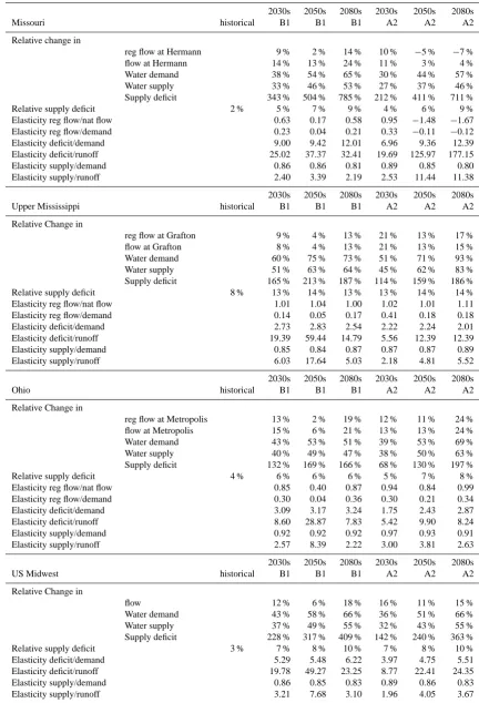
For evaluating future implications we refer to seasonal and annual relative changes in natural and regulated flows, de-mand, actual supply and supply deficit with respect to the historical period. We also identify drivers of change using (i) covariances of supply deficit with annual inflow and an-nual demand over different future periods, and (ii) elastici-ties with respect to changes in natural flow and changes in demand. The covariances quantify the impact of changes in natural flow and changes in demand on the supply deficit over our simulations. Larger covariances with respect to flow than

63 1

Figure 8: long term simulated time series of historical and future (B1) mean annual regulated and natural flow for the

2

three regions.

3

4 Fig. 7. long-term simulated time series of historical and future (B1) mean annual regulated and natural flow for the three regions.

with respect to demand support that the flow is the primary driving component for changes in supply deficit. The elastic-ities are the ratios of the relative changes in supply deficit, ac-tual supply or regulated flow, over the relative change in natu-ral flow or demand. Elasticities quantify the sensitivity of the variables to changes in predicted flow and demand and gener-alize the results on the identification of the drivers of change. Large elasticities indicate larger sensitivities and therefore the importance of the driver. Small differences in elastici-ties with respect to flow and demand indicate a balance in the drivers. Table 3 presents the relative change and elastic-ities metrics for the Missouri, Upper Mississippi, Ohio and the entire Midwest. Table 4 presents the covariances quanti-fying the reasons of change in supply deficit for the Missouri, Upper Mississippi and Ohio.

4.2.1 Demand and natural flows

Table 2. Percent change in annual discharge of the simulated regulated flow with respect to the simulated natural discharge.

Station Name B1 A2

historical 2030s 2050s 2080s 2030s 2050s 2080s

Missouri at Hermann −28 % −32 % −35 % −34 % −29 % −34 % −36 %

Upper Mississippi at Grafton −2 % −2 % −2 % −3 % −2 % −2 % −1 %

Ohio at Metropolis −8 % −10 % −11 % −10 % −9 % −10 % −9 %

US Midwest −10 % −11 % −13 % −12 % −10 % −11 % −10 %

64 1

Figure 9: Monthly average of total water demand (left), and supply deficit (right) over the three regions and over the

2

entire domain for different time periods.

3 4

Fig. 8. Monthly average of total water demand (left), and supply deficit (right) over the three regions and over the entire domain for different time periods.

GCAM projects the consumptive irrigation demand to keep increasing over the US Midwest while the non-irrigation consumptive demand increased at a very slow and approximately constant rate (Fig. 5a and b). With the frac-tion of irrigafrac-tion demand over the total demand decreasing over the Ohio and Upper Mississippi in the future (Table 5), the demand plateau over the two regions is associated with domestic and thermoelectric demands based on a population projected to stagnate by 2050 in the B1 and A2 scenarios. The steady increase in irrigation water withdrawal (Fig. 5) in the US Midwest is primarily attributed to the projected expansion of biomass, especially in the second half of the 21st century. One the other hand, the projected reduction in total non-irrigation water withdrawal is mainly attributed to the technological change of water cooling technologies for electricity generation (Fig. 5); i.e., the phasing out of

once-through cooling technology and the greater prevalence of more water efficient cooling technologies such as recir-culating towers and cooling ponds. Although the total wa-ter withdrawal results also encompass the effects of popula-tion growth, income effect, fuel mix, energy demand, and cli-mate mitigation, the effects of cooling technology dominated the direction of the change. Since recirculating technologies generally withdraw much less but consume more water than once-through cooling, the total consumptive use for non-irrigation, unlike withdrawals, shows a slight increase.

We force SCLM-MOSART with the downscaled GFDL B1 and GFDL A2 future meteorological forcings. Figure 10 shows the predicted naturalized flow due to climate change over the three regions. Figure 10 and Table 3 show the monthly and annual relative change of natural flow with re-spect to the historical simulations. The region is predicted to have a warmer climate and overall more precipitation, lead-ing to an overall increased annual natural flow, and higher snowmelt while summer flows decrease (Fig. 10). The in-creased annual flow, higher snowmelt and lower summer flow tend to be similar between the 2030s and 2050s but fur-ther accentuate by the 2080s. The effects of climate change on natural flow over the US Midwest are consistent with the findings of others (Mishra et al., 2010; CCSP, 2008).

We further force SCLM-MOSART-WM with the down-scaled GFDL B1 and A2 future meteorological forcing with GCAM demand corresponding to the downscaled GFDL B1 and GFDL A2 scenario emission climates.

4.2.2 Flow regulation

Figure 10 shows the projected mean monthly regulated flow for future periods and the relative change in regulated flow with respect to the historical regulated flows. The change in operations is not taken into account as operating rules are calibrated using the historical demands and flows (see discus-sion). The relative changes in monthly regulated flow (solid line) due to changes in climate (GFDL-B1, GFDL-A2) and demands (GCAM-B1 and GCAM-A2) are projected to be very close to the relative change in natural flow (dashed) due to climate change only over the Ohio and Upper Mississippi basins. The elasticities of the regulated flow with respect to natural flow and demand in Table 3 show that changes in reg-ulated flow over the Upper Mississippi are driven by changes

Table 3. Relative change in annual discharge, water demand, water supply and supply deficit with respect to the historical period. Elasticities of water supply and supply deficit to changes in demand or discharge with respect to the historical period.

2030s 2050s 2080s 2030s 2050s 2080s

Missouri historical B1 B1 B1 A2 A2 A2

Relative change in

reg flow at Hermann 9 % 2 % 14 % 10 % −5 % −7 %

flow at Hermann 14 % 13 % 24 % 11 % 3 % 4 %

Water demand 38 % 54 % 65 % 30 % 44 % 57 %

Water supply 33 % 46 % 53 % 27 % 37 % 46 %

Supply deficit 343 % 504 % 785 % 212 % 411 % 711 %

Relative supply deficit 2 % 5 % 7 % 9 % 4 % 6 % 9 %

Elasticity reg flow/nat flow 0.63 0.17 0.58 0.95 −1.48 −1.67

Elasticity reg flow/demand 0.23 0.04 0.21 0.33 −0.11 −0.12

Elasticity deficit/demand 9.00 9.42 12.01 6.96 9.36 12.39

Elasticity deficit/runoff 25.02 37.37 32.41 19.69 125.97 177.15

Elasticity supply/demand 0.86 0.86 0.81 0.89 0.85 0.80

Elasticity supply/runoff 2.40 3.39 2.19 2.53 11.44 11.38

2030s 2050s 2080s 2030s 2050s 2080s

Upper Mississippi historical B1 B1 B1 A2 A2 A2

Relative Change in

reg flow at Grafton 9 % 4 % 13 % 21 % 13 % 17 %

flow at Grafton 8 % 4 % 13 % 21 % 13 % 15 %

Water demand 60 % 75 % 73 % 51 % 71 % 93 %

Water supply 51 % 63 % 64 % 45 % 62 % 83 %

Supply deficit 165 % 213 % 187 % 114 % 159 % 186 %

Relative supply deficit 8 % 13 % 14 % 13 % 13 % 14 % 14 %

Elasticity reg flow/nat flow 1.01 1.04 1.00 1.02 1.01 1.11

Elasticity reg flow/demand 0.14 0.05 0.17 0.41 0.18 0.18

Elasticity deficit/demand 2.73 2.83 2.54 2.22 2.24 2.01

Elasticity deficit/runoff 19.39 59.44 14.79 5.56 12.39 12.39

Elasticity supply/demand 0.85 0.84 0.87 0.87 0.87 0.89

Elasticity supply/runoff 6.03 17.64 5.03 2.18 4.81 5.52

2030s 2050s 2080s 2030s 2050s 2080s

Ohio historical B1 B1 B1 A2 A2 A2

Relative Change in

reg flow at Metropolis 13 % 2 % 19 % 12 % 11 % 24 %

flow at Metropolis 15 % 6 % 21 % 13 % 13 % 24 %

Water demand 43 % 53 % 51 % 39 % 53 % 69 %

Water supply 40 % 49 % 47 % 38 % 50 % 63 %

Supply deficit 132 % 169 % 166 % 68 % 130 % 197 %

Relative supply deficit 4 % 6 % 6 % 6 % 5 % 7 % 8 %

Elasticity reg flow/nat flow 0.85 0.40 0.87 0.94 0.84 0.99

Elasticity reg flow/demand 0.30 0.04 0.36 0.30 0.21 0.34

Elasticity deficit/demand 3.09 3.17 3.24 1.75 2.43 2.87

Elasticity deficit/runoff 8.60 28.87 7.83 5.42 9.90 8.24

Elasticity supply/demand 0.92 0.92 0.92 0.97 0.93 0.91

Elasticity supply/runoff 2.57 8.39 2.22 3.00 3.81 2.63

2030s 2050s 2080s 2030s 2050s 2080s

US Midwest historical B1 B1 B1 A2 A2 A2

Relative Change in

flow 12 % 6 % 18 % 16 % 11 % 15 %

Water demand 43 % 58 % 66 % 36 % 51 % 66 %

Water supply 37 % 49 % 55 % 32 % 43 % 55 %

Supply deficit 228 % 317 % 409 % 142 % 240 % 363 %

Relative supply deficit 3 % 7 % 8 % 10 % 7 % 8 % 10 %

Elasticity deficit/demand 5.29 5.48 6.22 3.97 4.75 5.51

Elasticity deficit/runoff 19.78 49.27 23.25 8.77 22.41 24.35

Elasticity supply/demand 0.86 0.85 0.83 0.89 0.86 0.83

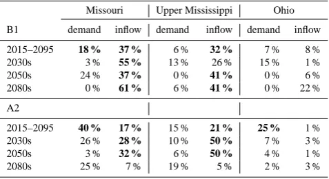
Table 4. Covariances of supply deficit with inflow and water de-mand. Bold values are significant at the 90 % confidence level.

Missouri Upper Mississippi Ohio

B1 demand inflow demand inflow demand inflow

2015–2095 18 % 37 % 6 % 32 % 7 % 8 %

2030s 3 % 55 % 13 % 26 % 15 % 1 %

2050s 24 % 37 % 0 % 41 % 0 % 6 %

2080s 0 % 61 % 6 % 41 % 0 % 22 %

A2

2015–2095 40 % 17 % 15 % 21 % 25 % 1 %

2030s 26 % 28 % 10 % 50 % 7 % 3 %

2050s 3 % 32 % 6 % 50 % 4 % 1 %

2080s 25 % 7 % 19 % 5 % 2 % 3 %

in natural flow and are of equal magnitude for both B1 and A2, with elasticities close to 1. Elasticities of regulated flow with respect to natural flow for the Ohio are lower for B1 but close to 1 for A2 as well. The changes in demand have effect on the regulated flows but are less than two to three times the impact of change in natural flow, as shown by the ratio of elasticities. Over the Missouri in July, August and September, starting in the 2050s, the change in regulated flow (climate and demand) is twice the magnitude, or same mag-nitude but of opposite effect, compared to the change in nat-uralized flow. The summer Missouri regulated flow is im-pacted by changes in natural flow and demand. On an an-nual timescale, changes in regulated flow over the Missouri are driven by changes in natural flow but not as much as the two other regions (covariances not shown). Elasticities with respect to natural flow and demand are also much closer to each other. Note, however, that the regulated flow is predicted to decrease in future period for A2. All Missouri elasticities with respect to natural flow in Table 3 increase tremendously as the system reaches its limit for actual supply so the natural flow also becomes the main driver of changes. Note also that the GCAM demand is not constrained by water availability.

4.2.3 Supply

Figure 8 shows the projected mean monthly water supply deficit over the Missouri, Upper Mississippi, Ohio, and Up-per Midwest. Figure 9 shows the change in relative water supply deficit, which characterizes the need for and the re-liance on an additional source of water supply in the future. The supply deficit is expected to keep increasing over the Missouri River basin, stagnate over the Ohio by the 2050s, and slow in its increase in the Upper Mississippi (Table 3). The largest demand being over the Missouri, the supply deficit over the entire Upper Midwest follows its increasing trend. The end of the summer is the most vulnerable period. In terms of the relative supply deficit and dependence on other source of supply, the Missouri is projected to experi-ence its dependexperi-ence jump from below 5 % to up to 15 % by 2080s for the month of September for both scenarios. The

65 1

Figure 10: relative change in total GCAM demand with respect to the historical demand for the three regions (left), and

2

regional mean monthly fractional water supply deficit – or reliance on another water supply- for historical and future

3

periods.

4 5

Fig. 9. relative change in total GCAM demand with respect to the historical demand for the three regions (left), and regional mean monthly fractional water supply deficit – or reliance on another wa-ter supply – for historical and future periods.

Missouri has the largest increase in annual relative supply deficit from 2 % for the historical period to 9 % by the 2080s in both scenarios, but the Upper Mississippi River basin has the largest dependencies, changing from 9 % historically to 14 % by the 2080s, for both scenarios as well (Table 3).

Table 4 shows the covariances of supply deficit with fu-ture natural flow and water demand for the Missouri, Up-per Mississippi and Ohio and both scenarios. Over the 2015– 2095 period, the supply deficit over the Missouri is explained by the future flow and the water demand because the supply deficit goes through a steady increase following the water de-mand pattern (Fig. 5). Over shorter time periods, the variance in supply deficit is explained by the flow. Noteworthy is that our water demand presently has no interannual variability but there is a steady increase in the long term. Interannual vari-ability should vary with global markets and water availvari-ability that will be the object of the two-way coupling in progress. Over the Upper Mississippi, the supply deficit is driven by the flow given the low storage capacity. Over the Ohio River basin there is no significant covariance except with water de-mand over a long period with the A2 scenario. Like the Up-per Mississippi, the storage capacity is limited over the Ohio and the flow would be expected to drive the supply deficit. However, the water demand over the Ohio is mostly for non-irrigation use and is more localized. The low covariances are due to the specificity of the Ohio region, with the available

Table 5. Fraction of total demand attributed to the irrigation sector.

Period

B1 A2

Midwest Missouri Ohio Upper Midwest Missouri Ohio Upper

Mississippi Mississippi

Hist 0.8 0.9 0.35 0.75 0.8 0.9 0.35 0.75

2030s 0.82 0.9 0.44 0.8 0.83 0.9 0.42 0.79

2050s 0.84 0.92 0.47 0.81 0.85 0.91 0.47 0.81

2080s 0.85 0.93 0.42 0.71 0.76 0.81 0.46 0.74

water not reachable by the demanding areas, as shown next. Similarly, the lack of interannual variability in the demand explains the low covariance of supply deficit with demand over shorter periods.

Figure 11 displays the spatial distribution of the GCAM annual consumptive water demand, the simulated SCLM-MOSART-WM water supply, and the corresponding relative supply deficit for the historical and B1 future periods. The GCAM demands are projected to increase in particular over the Platte River and urban area over the Ohio and Upper Mississippi river basins. The supply increases where the de-mand increases. However, the supply deficit does not obvi-ously overlay the regions with the highest demand, but rather seems to reflect a combination of demand and water avail-ability, i.e., upstream of the Osage River and the urban areas adjacent to the Great Lakes.

5 Discussion

In view of the results and methodology, we highlight three areas of discussion: (i) the sensitivity of the integrated mod-eling results with respect to hydrologic and other modmod-eling errors; (ii) drivers of change in projected stream discharge and ability to meet the water demand; and (iii) reconciliation of SCLM and GCAM water balances through the input of withdrawals in addition to consumptive demand, groundwa-ter supply, and full coupling between WM and SCLM and water allocation when demands exceed water availability.

5.1 Modeling errors

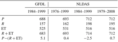
The SCLM-MOSART simulations driven by the downscaled GFDL historical climate produced an overall underestima-tion of the observed naturalized flow at Hermann. Table 6 shows the regional water balance of the GFDL-SCLM-MOSART simulations compared to the SCLM-GFDL-SCLM-MOSART simulations driven by the NLDAS2 forcing data. The down-scaled GFDL climate is drier and has higher net radiation compared to NLDAS2, with the differences larger in 1984– 1999 than 1976–1999. This results in lower runoff in GFDL-SCLM-MOSART than NLDAS-GFDL-SCLM-MOSART. The bias in the downscaled GFDL climate is not surprising, as very little constraints are used in the global climate simulations.

Table 6. Water balance comparison of GFDL against NLDAS (P=precipitation;R=total runoff; ET=evapotranspiration) for the Upper Midwest region.

GFDL NLDAS

1984–1999 1976–1999 1984–1999 1979–2008

P 688 693 712 712

R 157 162 198 195

ET 525 531 516 516

R+ET 683 693 714 712

P−(R+ET) 5.1 0.4 −2.5 0.7

Even statistical downscaling methods such as the constructed analog cannot fully remove the biases in the climate simu-lations. Using an ensemble of climate models may reduce the overall biases, but this is beyond of the scope of this study. The runoff coefficients, however, are similar to those extracted from the Maurer et al. (2002) simulations, which are often used as reference. Despite the simulation biases, the numerical experiments reported here showed proof of con-cept in one-way coupling of a terrestrial system model that includes a land surface model, river routing model and water resources management with a water demand model, which is part of a global integrated assessment model. Our results showed reasonable agreement in simulating the effect of hu-man activities on the land surface system.

66 1

Figure 11: Left column: Simulated mean monthly natural (dashed) and regulated (solid) flow at Hermann, Grafton and 2

Metropolis for different time period: historical (98-99), 2030s B1(2015-45), 2050s B1(2035-2065) and 2080s B1(2065-3

2095).Right column: relative change in mea mean monthly flow of natural (dashed) and regulated (solid) flow for future 4

B1 periods with respect to their historical counterparts. Close monthly relative changes between natural and regulated 5

flow with the A2 emission scenario were also observed. 6

Fig. 10. Left column: simulated mean monthly natural (dashed) and regulated (solid) flow at Hermann, Grafton and Metropolis for dif-ferent time periods: historical (1998–1999), 2030s B1 (2015–2045), 2050s B1 (2035–2065) and 2080s B1 (2065–2095). Right column: relative change in mean monthly flow of natural (dashed) and regu-lated (solid) flow for future B1 periods with respect to their histori-cal counterparts. Results with A2 emission scenario were similar.

a function of changes in monthly natural flow and storage capacity over the region and reservoir uses.

5.2 Drivers of change in future human effects on land

surface system

The human activities are represented by a water management model and a global integrated assessment model that simu-lates water demand. Rainfed crop demand is handled directly by the land surface modeling component. We investigate the drivers of the change in regulated flow and supply deficit us-ing covariances (Table 4) and elasticities (Table 3) with re-spect to climate-induced change in natural flow and changes in water demand driven by socioeconomic factors, energy and food demands, global markets and prices. Figure 12 also presents scatterplots of annual change in regulated discharge and annual relative change in supply deficit.

Over the Ohio River basin, the demand is localized over specific urban areas (Fig. 11) and exceeds the locally avail-able water. Cities might be located too far from the main stem from which they could request water from reservoir releases. Mostly, the reservoir storage along the main stem does not al-low much regulation at the monthly timescale (Figs. 1, 6 and 7). Because of the limited storage capacity of the reservoirs over the Ohio River, a relatively low demand, and cities with high demand but too far from the main stem to access the water supply according to our database rules, climate change effects on the natural flow drive the change in regulated flow

(Fig. 9) with changes being of about equal magnitude (elas-ticities close to 1). Changes in supply deficit are driven by changes in demand regionally but are driven by a combi-nation of changes in runoff and demand locally around the high demand urban areas. For B1, the elasticity of the supply deficit with respect to changes in demand stagnates around 3. Relative to changes in flow, the elasticity is more uncer-tain, with a higher range of fluctuation between 5.4 and 28.9. However, supply deficit over the Ohio is the least sensitive to changes in flow and demand than the other regions (Fig. 12 and Table 4).

Over the Upper Mississippi River basin, the increase in de-mand with increasing supply deficit is localized over the ur-ban and agricultural areas adjacent to the Great Lakes. There are cities like St. Louis along the main stem that actually have very small, or almost no supply deficit (Fig. 11). Changes in regulated flow are driven by changes in natural flow, with elasticities close to 1 (Table 3) due to the limited storage ca-pacity, relatively low demand with respect to the annual flow and cities and fields too far from the main stem, like over the Ohio River basin. Elasticities with respect to changes in demand are small (between 0.05 and 0.41). The increases in supply deficit are driven primarily by the change in runoff, as seen in Fig. 12 and Table 4. Elasticities of supply deficit with respect to flow, however, are more uncertain as they range between 5 and 60, while elasticities with respect to demand stagnate between 2 and 3.

Over the Missouri River basin, the increase in demand is spread out with a large demand along the Platte River valley (Fig. 11). However, the supply deficit is mostly localized over the headwaters of the Platte River. As seen in Voisin et al. (2013), an excessive surface water demand can drive upstream reservoir dry leaving headwater areas with a sup-ply deficit. The area is relying significantly on groundwater pumping with 26 %, 11 %, 7 % of withdrawals over the Mis-souri and Upper Mississippi and Ohio respectively coming from groundwater, although how much groundwater comes from confined aquifers has not been specified (Kenny et al., 2009). Voisin et al. (2013) recommend to adjust the with-drawals and consumptive use demand on the surface water system for groundwater. The sensitivity to the fraction of irri-gation groundwater use is the focus of further research. With regulated runoff being affected by a combination of change in natural flow and in demand (Fig. 9), Fig. 12 links the change in supply deficit to the change in regulated runoff, i.e., changes in natural flow and demand. The supply deficit over the Missouri is controlled mostly by the natural flow over shorter periods and demand over longer periods (Ta-ble 4). The Missouri is the most sensitive to changes in runoff and demand, showing the largest elasticities with respect to both flow and demand. The change in runoff is still the pre-dominant driver of the change in supply deficit, especially under A2 when the system seems to reach its supplying limit. However, sensitivity of supply deficit to changes in demand should be taken into consideration for climate change impact

67 1

2

Figure 12: Annual total water demand (left) and actual water supply (center) in cubic meters, and fractional water supply

3

deficit for historical and future B1 periods.

4

5

Fig. 11. Annual total water demand (left) and actual water supply (center) in cubic meters, and fractional water supply deficit for historical and future B1 periods.

assessment given that about 21 % of the annual flow is con-sumed.

For the US Midwest, it is important to note that supply deficit is around six times as sensitive to changes in runoff and demand than the actual supply; it increases to 10 times over the Missouri and decreases to 3 times over the Ohio and Upper Mississippi. This emphasizes the predicted com-petition between water uses in the future and the importance to look at the water demand driven by socioeconomics fac-tors and global markets. It is also noteworthy to look at the range of elasticities of the supply deficit with respect to flow and demand over future periods and between a pessimistic A2 scenario and an optimistic B1 scenario, in particular from 2050s to 2080s when the A2 and B1 climate scenarios tend to significantly diverge. The range of elasticities show the com-plex interactions between changes in climate-induced natural flow, socioeconomics changes in water demand, the storage capacity of the region and the reservoir model regulation and extraction.

5.3 Water balance

GCAM uses an independent model different from SCLM to simulate water balance so GCAM’s estimates of water demands may be inconsistent with the water availability in SCLM. This can be resolved once a two-way (full) coupling between GCAM and SCLM-MOSART-WM is established, where the latter provides the amount of water availability and thus constraining water demands in GCAM (Tamea et al., 2013; Konar et al., 2013). However, we also need to quan-tify how much groundwater comes from unconfined aquifer

and how much comes from return flow for adjusting the de-mand on the surface water system. Similarly, in order to use withdrawals more research focused on the full coupling of the water resources management model with the land surface hydrology model is needed.

6 Conclusions

4572 N. Voisin et al.: Evaluation and implications of future changes over the US Midwest

68 2

3

4

Figure 13: Relationship between total annual regulated runoff and percent deficit of annual water demand for the

5

historical and future B1 (black diamonds) and A2 (red cross) simulations, over the three regions and the Upper Midwest.

6

7

8

9

10

11

Fig. 12. Relationship between total annual regulated runoff and percent deficit of annual water demand for the historical and future B1 (black diamonds) and A2 (red cross) simulations, over the three regions and the Upper Midwest.

a. Over the historical period, the integrated system is rea-sonably well reproducing the anthropogenic influence on the flow and the water supply over the three regions. b. Implications for future water resources affected by the human influence are driven by changes in the water demands simulated by GCAM and the change in flow (climate change). With the Upper Midwest projected (GFDL-B1 and GFDL-A2) to have an increased in an-nual flow and in particular snowmelt flows.

c. There is uncertainty in the direction of the mean annual regulated flow. The annual regulated flow is projected to slightly increase with B1 but decrease with A2. Sea-sonally, the regulated flow is projected to increase over the snowmelt period (A2 and B1) and remain similar (B1) or lower (A2) to historical regulated flow during the summer.

d. The actual supply is also projected to increase but not enough to compensate for the increase in demand, i.e., the relative supply deficit is projected to increase over the region. The largest relative supply deficit is simu-lated over the Upper Mississippi.

e. Drivers of the changes in regulated flow are the changes in the natural flow due to climate change for the Ohio and Upper Mississippi, and a combination of changes in socioeconomic factors that drive changes in water demand and climate change that drives changes in natural flow over the Missouri Over the Missouri, both changes in flow and demand need to be taken into consideration for projecting future water resources. f. Supply deficit is 6 times more sensitive to changes in

natural flow and demand than water supply is. Drivers

of the change in supply deficit are the changes in natu-ral flow over the US Midwest in genenatu-ral, and over the Upper Mississippi. The change in supply deficit over the Ohio is driven by the change in demand that is very localized around urban areas. The change in sup-ply deficit over the Missouri, however, is driven by a combination of change in demand and in natural flow. Over the US Midwest where the natural flow is projected to increase and the crop is mostly rain fed, changes in regulated flow and supply, and supply deficit are driven by the change in runoff due to climate change, more than the change in so-cioeconomic water demands. Regionally, however, the mod-eling of water demands allows us to isolate sectors and areas that will be more sensitive to change in demand and will rely on groundwater and virtual water trade. Over areas relying more heavily on irrigation, we anticipate a stronger signal between the change in demand and change in supply deficit and flow regulation. The sensitivity analysis of supply deficit with respect to changes in flow and demand shows the com-plex interactions between changes in climate-induced natural flow, socioeconomics changes in water demand, the storage capacity of the region and the reservoir model regulation and extraction. The study presents a successful one-way coupling of a global integrated assessment model with a regional scale hydrologic and water management model. Future work will focus on the effect of hydrologic errors and on updating the reservoir module operating rules over more regions.

Acknowledgements. The authors would like to thank S. Siebert at

the University of Bonn, Germany for providing the global gridded monthly irrigation water requirements data for crops, and Duane Ward at the Pacific Northwest National Laboratory (PNNL) for his assistance with the WM dependence database set up over the US