A Bayesian joint probability post processor for reducing errors and quantifying uncertainty in monthly streamflow predictions

(1)

Hydrol. Earth Syst. Sci., 17, 795–804, 2013 www.hydrol-earth-syst-sci.net/17/795/2013/ doi:10.5194/hess-17-795-2013

EGU Journal Logos (RGB)

Advances in

Geosciences

Open Access

Natural Hazards

and Earth System

Sciences

Open Access

Annales

Geophysicae

Open Access

Nonlinear Processes

in Geophysics

Open Access

Atmospheric

Chemistry

and Physics

Open Access

Atmospheric

Chemistry

and Physics

Open Access

Discussions

Atmospheric

Measurement

Techniques

Open Access

Atmospheric

Measurement

Techniques

Open Access

Discussions

Biogeosciences

Open Access Open Access

Biogeosciences

Discussions

Climate

of the Past

Climate

of the Past

Discussions

Earth System

Dynamics

Earth System

Dynamics

Discussions

Geoscientific

Instrumentation

Methods and

Data Systems

Open Access

_{Geoscientific}

Instrumentation

Methods and

Data Systems

Open Access

Discussions

Geoscientific

Model Development

Geoscientific

Model Development

Discussions

Hydrology and

Earth System

Sciences

Open Access

Hydrology and

Earth System

Sciences

Open Access

Discussions

Ocean Science

Discussions

Solid Earth

Discussions

The Cryosphere

Discussions

Natural Hazards

and Earth System

Sciences

Open Access

Discussions

A Bayesian joint probability post-processor for reducing errors

and quantifying uncertainty in monthly streamflow predictions

P. Pokhrel, D. E. Robertson, and Q. J. Wang

CSIRO Land and Water, Graham Road, Highett, Victoria, Australia

Correspondence to: P. Pokhrel ([email protected])

Received: 7 September 2012 – Published in Hydrol. Earth Syst. Sci. Discuss.: 2 October 2012 Revised: 9 January 2013 – Accepted: 25 January 2013 – Published: 22 February 2013

Abstract. Hydrologic model predictions are often biased

and subject to heteroscedastic errors originating from vari-ous sources including data, model structure and parameter calibration. Statistical post-processors are applied to reduce such errors and quantify uncertainty in the predictions. In this study, we investigate the use of a statistical post-processor based on the Bayesian joint probability (BJP) modelling ap-proach to reduce errors and quantify uncertainty in stream-flow predictions generated from a monthly water balance model. The BJP post-processor reduces errors through elim-ination of systematic bias and through transient errors up-dating. It uses a parametric transformation to normalize data and stabilize variance and allows for parameter uncertainty in the post-processor. We apply the BJP post-processor to 18 catchments located in eastern Australia and demonstrate its effectiveness in reducing prediction errors and quantifying prediction uncertainty.

1 Introduction

Streamflow predictions from a hydrological model can be used for wide range of applications including flood forecast-ing at short time scales to long-term assessments of water resources. Model predictions are subject to errors originating from various sources including input data, model structure and parameters. The model is usually calibrated prior to its application to compensate for these errors, thus reducing un-certainty in the predictions. However, a model being a sim-plified representation of a system will always contain uncer-tainty in its predictions (Gupta et al., 2005). Post-processors are statistical models that are applied to model predictions

to further reduce errors and to quantify uncertainty in the streamflow predictions (Seo et al., 2006).

Post-processors can reduce errors through elimination of systematic bias and/or by reduction of “short memory” or transient errors (Pagano et al., 2011). The former is generally achieved by using simple statistical approaches like quantile mapping or regression (Hashino et al., 2007; Shi et al., 2008), while the latter is generally achieved by prediction updating (Lekkas et al., 2001; Moraweitz et al., 2011). The prediction updating techniques exploit persistence of residuals to cor-rect for errors using linear or non-linear auto-regressive mod-els (WMO, 1992; Shamseldin and O’Connor, 2001; Xiong and O’Connor, 2002; Pagano et al., 2011). Streamflow pre-dictions, even after bias correction and prediction updat-ing, contain errors that cannot be eliminated, and informa-tion on predicinforma-tion uncertainty is useful for decision makers who use the predictions. Post-processors are generally de-signed to provide an estimate of the total “lumped” uncer-tainty in the predictions by constructing statistical models of errors based on model predictions and historical observations (e.g. Krzysztofowicz, 1999; Engeland et al., 2005; Montanari and Grossi, 2008).

(2)

796 P. Pokhrel et al.: A Bayesian joint probability post-processor

distributions. Some are primarily intended for uncertainty quantification but also include components for error reduc-tion (e.g. Krzysztofowicz, 1999, 2002).

Methods for parameterization, parameter estimation and calculation of predictive distributions differ among post-processors, although some common features can be found. Most post-processors produce probabilistic predictive distri-butions of streamflow (or river height) conditioned on model predictions and recent streamflow observations. They gener-ally assume linear dependence among the variates in a formed normal space, and most use normal quantile trans-formation (NQT; Krzysztofowicz, 1997, 1999; Todini, 2008; Li et al., 2010) to normalize the variables. All assume the estimated values of the parameters (of the post-processors) to be “true” and ignore the uncertainty in estimating their values (Krzysztofowicz, 1999, 2002). For a complex post-processor like BFS, this (parametric uncertainty) can be sub-stantial (Seo et al., 2006). More importantly, they are all de-signed to post-process streamflow predictions at daily or sub-daily time scales.

For many hydrological applications, such as seasonal streamflow forecasting, water resources and climate change assessments, monthly streamflow volumes are of primary interest. While daily predictions from daily models may be post-processed at the daily time scale and then aggre-gated to monthly, there is no guarantee that the monthly volumes so produced have reliable uncertainty distributions and the least errors achievable. It is likely much more ef-fective to apply post-processing directly at the monthly time scale, where pre-processed monthly volumes may come ei-ther from aggregating daily model outputs or simply from monthly models.

In this study, we investigate the use of a Bayesian joint probability (BJP) modelling approach to post-process model predictions of monthly streamflow volumes. The BJP method was originally developed for forecasting seasonal stream-flows in Australia (Wang et al., 2009). Here we apply it for bias correction, prediction updating and uncertainty quan-tification of monthly streamflow volumes generated from a monthly water balance model. The BJP method uses a parametric transformation to normalize data and stabilize variance. It allows for parameter uncertainty in the post-processor, and this can be important when dealing with monthly variables, which have far fewer data points than daily variables. In this study, we assess three formulations of the BJP post-processor in their ability to reduce error and quantify uncertainty.

The paper is structured as follows. Section 2 describes the catchments and data used in the study. Section 3 presents the hydrological model used and the formulations of the BJP post-processor. Evaluation of the post-processor is given in Sect. 4 and followed by discussions in Sect. 5. Conclusions are drawn in Sect. 6.

2 Study area and data

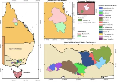
We test BJP post-processor in 18 catchments located in Queensland, Victoria (including one at the border with New South Wales) and Tasmania (see Fig. 1). The Victorian catch-ments are further divided into 3 regions: upper Murray, cen-tral Victoria and southern Victoria (see Table 1).

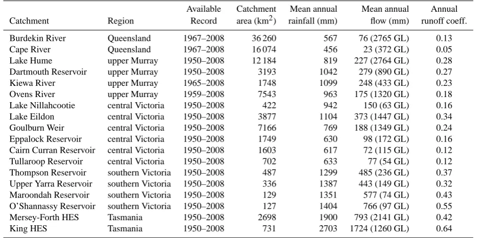
The catchments range in size from 127 to 36 000 km2. The Queensland catchments are the largest in size and experi-ence a semi-arid type of climate, characterized by low rain-fall and high evapotranspiration. The mean annual rainrain-fall is less than 600 mm, and the catchments are dry during the aus-tral winter. In contrast, the Victorian catchments experience a temperate climate, with higher rainfall (617–1400 mm) oc-curring during the austral winter and spring. The Tasmanian catchments experience temperate oceanic climate and are the wettest with mean annual rainfall in excess of 1900 mm. The Tasmanian catchments are wet throughout the year.

We use observed monthly streamflow data obtained from various water resource management agencies and the Bu-reau of Meteorology, Australia. For most catchments, with the exception of some in Queensland and Victoria, the data are available from 1950 to 2008 (see Table 1). The monthly catchment average rainfall and potential evapotran-spiration for each catchment are calculated from a 5-km grid-ded dataset available from the Australian Water Availability Project (AWAP; Jones et al., 2009).

3 Methods

In each catchment, we calibrate parameters of a hydro-logic water balance model and generate streamflow pre-dictions. In the context of this study, we define prediction as one time step ahead of forecast of streamflow, under perfect rainfall forecast. The “raw” deterministic stream-flow predictions generated by the model contain errors that are unreconciled during calibration process. The BJP post-processor aims to reduce such errors and quantify un-certainty. This section describes the process of generating streamflow predictions, using a hydrologic model, and their subsequent post-processing.

3.1 Generation of streamflow predictions using a hydrological model

(3)

[image:3.595.64.538.82.315.2]

Table 1. Brief attributes of the 18 catchments used for the study.

Available Catchment Mean annual Mean annual Annual Catchment Region Record area (km2) rainfall (mm) flow (mm) runoff coeff.

Burdekin River Queensland 1967–2008 36 260 567 76 (2765 GL) 0.13

Cape River Queensland 1967–2008 16 074 456 23 (372 GL) 0.05

Lake Hume upper Murray 1950–2008 12 184 819 227 (2764 GL) 0.28

Dartmouth Reservoir upper Murray 1950–2008 3193 1042 279 (890 GL) 0.27

Kiewa River upper Murray 1965–2008 1748 1099 248 (433 GL) 0.23

Ovens River upper Murray 1959–2008 7543 963 175 (1320 GL) 0.18

Lake Nillahcootie central Victoria 1950–2008 422 942 150 (63 GL) 0.16 Lake Eildon central Victoria 1950–2008 3877 1104 373 (1447 GL) 0.34 Goulburn Weir central Victoria 1950–2008 7166 769 188 (1349 GL) 0.24 Eppalock Reservoir central Victoria 1950–2008 1749 630 98 (172 GL) 0.16 Cairn Curran Reservoir central Victoria 1950–2008 1603 617 72 (115 GL) 0.12 Tullaroop Reservoir central Victoria 1950–2008 702 633 77 (54 GL) 0.12 Thompson Reservoir southern Victoria 1950–2008 487 1299 485 (236 GL) 0.37 Upper Yarra Reservoir southern Victoria 1950–2008 336 1387 443 (149 GL) 0.32 Maroondah Reservoir southern Victoria 1950–2008 129 1351 577 (74 GL) 0.43 O’Shannassy Reservoir southern Victoria 1950–2008 127 1404 766 (97 GL) 0.55

Mersey-Forth HES Tasmania 1950–2008 2698 1900 793 (2141 GL) 0.42

King HES Tasmania 1950–2008 731 2703 1724 (1260 GL) 0.64

Note: HES stands for Hydro Electric Scheme.

We calibrate WAPABA using the shuffled complex evo-lution search method (SCE; Duan et al., 1994) for a pe-riod of five years. Prior to every model run we allow a five-year warm-up period to reduce model sensitivity to state ini-tialization errors. We maximize a scalarized multi-objective measure consisting of a uniformly weighted average of the Nash–Sutcliffe efficiency (NS) coefficient (Nash and Sut-cliffe, 1970), the NS of log transformed flows, the Pearson correlation coefficient and a symmetric measure of bias. The NS is an “observed-variance-normalized mean squared er-ror” measure that emphasizes large errors, often occurring during large events. The NS of log-transformed flow empha-sizes errors occurring during low flow events. The Pearson correlation measures the co-variability of the simulated and the observed. The symmetrical measure of bias evaluates the match between average simulation and average observation (Wang et al., 2011). We then use the calibrated parameters to produce raw WAPABA streamflow predictions using the observed rainfall.

3.2 Statistical post-processing

The BJP modelling approach assumes that a set of predic-tands,y(2), and their predictors,y(1), follow a joint multi-variate normal distribution in a transformed space. Normal-ization of the variables is achieved by using the log-sinh transformation (Wang et al., 2012). The log-sinh tion replaces the previously used Yeo-Johnson transforma-tion (Yeo and Johnson, 2000; Wang et al., 2009; Wang and Robertson, 2011). Although both have data normalization and variance stabilization properties, the log-sinh has been

shown to outperform the Box-Cox-based Yeo-Johnson trans-formation when applied to catchments with highly skewed data (Wang et al., 2011). The posterior distribution of the pa-rametersp(θ|YOBS), including mean, variance and

transfor-mation parameters for each variable and a correlation matrix for the multivariate normal distribution, is estimated using a Bayesian inference (Eq. 1):

p (θ|YOBS)∝p(θ)·p(YOBS|θ) (1)

whereYOBScontains the historical data of both predictory(1) and predictandy(2) variables used for model inference, and

θ is the parameter vector.p (θ)is the prior distribution of the parameters of the multivariate normal distribution, repre-senting any information available before the use of historical data,YOBS. The termp (YOBS|θ)is the likelihood function

defining the probability of observing the historical data given the model and the parameter sets. The posterior parameter distribution is approximated by 1000 sets of parameters sam-pled using a Markov Chain Monte Carlo (MCMC) method.

The posterior predictive density for a new event is given by

f (y (2)|y (1))=p (y (2)|y (1);YOBS) =

Z

p (y (2)|y (1) ,θ)·p(θ|YOBS)·dθ. (2)

(4)

17 454

Figure 1: Location of the 18 catchments used for the study.

455

155°0'0"E 155°0'0"E

150°0'0"E 150°0'0"E

145°0'0"E 145°0'0"E

2

0

°0

'0

"S

2

0

°0

'0

"S

3

0

°0

'0

"S

3

0

°0

'0

"S

4

0

°0

'0

"S

4

0

°0

'0

"S

148°0'0"E 147°0'0"E

146°0'0"E 145°0'0"E

144°0'0"E

3

6

°0

'0

"S

3

7

°0

'0

"S

CCN

DTM

EIL

EPP

GBLWR

HUM

KWA

MDH

NIL

OSH

OVN

THM

TUL

UYR

147°0'0"E 146°0'0"E 145°0'0"E 144°0'0"E

1

8

°0

'0

"S

1

9

°0

'0

"S

2

0

°0

'0

"S

2

1

°0

'0

"S

2

°0

'0

"S

BRD CPE

Victoria / New South Wales Catchments Queensland Catchments

New South Wales

Victoria

Tasmania Queensland

Burdekin R. Cape R.

Cairn Curran Rs. Dartmouth Rs. L. Eildon L. Eppalock Goulburn W. L. Hume Kiewa R. Maroondah Rs. L. Nillahcootie O' Shannassy Rs. Ovens R.

Thompsons Rs. Tullaroop Rs. Upper Yarra Rs.

146°0'0"E

4

2

°0

'0

"S

Queensland KNG MFT

Victoria / New South Wales

King H.E.S. Mersey-Forth H.E.S. Tasmania

Tasmania Catchments

Fig. 1. Location of the 18 catchments used for the study.

3.2.1 Method A

Method A represents the simplest case where only WAPABA predictions are applied as the predictor (y(1) in Eq. 2) and the observed streamflows as the predictand (y(2) in Eq. 2). This combination is to achieve two post-processing objec-tives, correction of systematic bias and quantification of un-certainty. The bias correction is achieved through the regres-sion property embedded within the BJP modelling approach (see Wang et al., 2009).

3.2.2 Method B

For method B, we add a second predictor over that used for method A. We add streamflow data observed one month pre-viously. The inclusion of lagged streamflow observations is to add an auto-regressive component to the post-processor and allow prediction updating. This method reduces errors through prediction updating as well as correction of system-atic bias and quantifies uncertainty.

3.2.3 Method C

For method C, we introduce a third predictor, the WAPABA model outputs simulated in the previous month. This inclu-sion is to further improve the prediction updating ability of the post-processor by utilizing the persistence in the simu-lated time series.

For each method, we first train the post-processor using the historically observed data. To account for seasonal ef-fects, we establish 12 different models for different months of the year. For each month, the post-processed probabilistic predictions are generated using a “leave-one-out” cross val-idation procedure. This consists of sampling the parameters using all but the year of interest and then generating predic-tions for the “left-out” year. The cross validation period in most catchments is about 59 yr (1950–2008).

Figure 2 is an example of the post-processed predictions generated by the BJP post-processor. This example is to provide the reader with an appreciation of how the post-processed predictions from the BJP post-processor may look. A detailed evaluation of the post-processor, with respect to the post-processing qualities, will be presented in Sect. 4. The example is drawn from Lake Eildon in central Victoria and shows [0.1, 0.25, 0.5, 0.75, 0.9] quantiles and observed streamflow values plotted chronologically. In this case the post-processed predictions do not show any obvious trend with time, and the widths of the quantile intervals seem to cover the expected number of observed values.

4 Results

[image:4.595.99.497.65.346.2]

(5)

P. Pokhrel et al.: A Bayesian joint probability post-processor 799

18 456

457

458

459

460

461

Figure 2: The time series of the post-processed prediction quantiles against the observed; only a

462

subset of the entire cross validation period is shown. [Light blue lines represent 0.1 – 0.9 quantiles,

463

dark blue lines represent the 0.25 – 0.75 quantiles, and blue dots represent the medians of the

post-464

processed predictive distributions. Red dots are the observed streamflow values.]

465

466

467

468

469

470

471

1990 1994 1998 2002 2006

0

5

0

1

0

1

5

0

2

0

Year

P

re

d

ic

ti

o

n

q

u

a

n

ti

le

r

a

n

g

e

s

&

o

b

s

e

rv

e

d

(

m

)

Fig. 2. The time series of the post-processed prediction quantiles

against the observed; only a subset of the entire cross validation period is shown (Light blue lines represent 0.1–0.9 quantiles, dark

blue lines represent the 0.25–0.75 quantiles, and blue dots represent the medians of the post-processed predictive distributions. Red dots are the observed streamflow values.).

how effective the BJP post-processor is in reducing errors and quantifying uncertainty.

4.1 Reduction of error

We assess the ability of the BJP post-processor to reduce er-rors by using a measure of accuracy called root mean squared error in probability (RMSEP; Wang and Robertson, 2011). RMSEP (Eq. 2) measures error in a probability space. An advantage of RMSEP over the more commonly used mean squared error or root mean squared error is that it places equal emphasis on errors obtained at all events rather than on a few large errors occurring at large events.

RMSEP=

"

1

n n

X

t=1

FCLI yt−FCLI(yOBSt )

2 #1₂

(3)

whereyt and y_OBSt are the predictions and observations at

t=1, 2. . .nevents respectively. The predictions can be ei-ther WAPABA simulations or the medians of post-processed distributions.FCLI is the cumulative historical distribution,

andFCLI(y)is the non-exceedance probability.

4.1.1 Performance of the WAPABA model

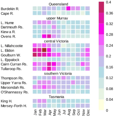
The RMSEP error values of the WAPABA predictions are shown in Fig. 3. Each row in the figure corresponds to a catchment and each column to a month. In general, except for Cape River and in Queensland, Thompson and O’Shannassy reservoirs in southern Victoria, the RMSEP values are rela-tively higher in drier months or months when the catchments just start to get wet. This occurs during August–October in Queensland, May–March in upper Murray, January–May in central Victoria and February–March in Tasmania.

19 473

474

475

476

Figure 3: Performance of WAPABA in all 18 catchments in terms of RMSEP values calculated for 477

each month. 478

479

480

J

a

n

F

e

b

M

a

r

A

p

r

M

a

y

J

u

n

J

u

l

A

u

g

S

e

p

O

c

t

N

o

v

D

e

c

Mersey-Forth H. King H.

O’Shannassy Rs. Maroondah Rs. Upper Yarra Rs. Thompson Rs.

Tullaroop Rs. Cairn Curran Rs. L. Eppalock Goulburn W. L. Eildon L. Nillahcootie

Ovens R. Kiew a R. Dartmouth Rs. L. Hume Cape R. Burdekin R.

Queensland

upper Murray

central Victoria

southern Victoria

Tasmania

0 0.04 0.08 0.12 0.16 0.2 0.24 0.28 0.32 0.36 0.4

Fig. 3. Performance of WAPABA in all 18 catchments in terms of

RMSEP values calculated for each month.

This suggests an inability of the model to properly charac-terize low flows and to capture the change in catchment dy-namics from being dry to getting wet. There can be various reasons for this, including, for example, non-consistency in the data between the calibration and evaluation period (with the calibration period being either wetter or drier), the choice of objective function for calibration, inadequate model struc-ture or a combination of these. While it might be interesting to investigate the causes of poor model performance in these catchments from a model diagnostic point of view, this is be-yond the scope of this study. Here we only focus on evaluat-ing whether the errors can be reduced by the post-processor.

4.1.2 Method A: bias reduction

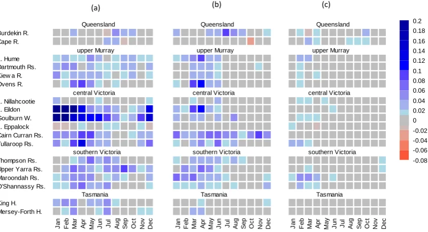
Figure 4a shows the differences in RMSEP error values be-tween the WAPABA predictions and those produced from method A (WAPABA prediction – method A). The values are colour coded with blue indicating the reductions in RMSEP error values and red indicating increases.

[image:5.595.50.286.62.208.2] [image:5.595.309.547.63.305.2]

(6)

20 481

482

Figure 4: (a) Difference in RMSEP values between WAPABA predictions and method A (WAPABA – method A); (b) difference in RMSEP values between

483

method A and B (method A –method B); (c) difference in RMSEP values between method B and C (method B – method C).

484

485

486

J

a

n

F

e

b

M

a

r

A

p

r

M

a

y

J

u

n

J

u

l

A

u

g

S

e

p

O

c

t

N

o

v

D

e

c

Mersey-Forth H. King H.

O’Shannassy Rs. Maroondah Rs. Upper Yarra Rs. Thompson Rs.

Tullaroop Rs. Cairn Curran Rs. L. Eppalock Goulburn W. L. Eildon L. Nillahcootie Ovens R. Kiew a R. Dartmouth Rs. L. Hume Cape R. Burdekin R.

Queensland

upper Murray

central Victoria

southern Victoria

Tasmania

J

a

n

F

e

b

M

a

r

A

p

r

M

a

y

J

u

n

J

u

l

A

u

g

S

e

p

O

c

t

N

o

v

D

e

c

Queensland

upper Murray

central Victoria

southern Victoria

Tasmania

J

a

n

F

e

b

M

a

r

A

p

r

M

a

y

J

u

n

J

u

l

A

u

g

S

e

p

O

c

t

N

o

v

D

e

c

Queensland

upper Murray

central Victoria

southern Victoria

Tasmania

-0.08 -0.06 -0.04 -0.02 0 0.02 0.04 0.06 0.08 0.1 0.12 0.14 0.16 0.18 0.2

(a) (b) (c)

Fig. 4. (a) Difference in RMSEP values between WAPABA predictions and method A (WAPABA – method A); (b) difference in RMSEP

values between method A and B (method A –method B); (c) difference in RMSEP values between method B and C (method B – method C).

4.1.3 Method B: prediction updating

Figure 4b shows the benefit of prediction updating by assimilating the recent streamflow observations (method B). We use the difference between methods A and B (method A – method B) to indicate any further reduc-tions in errors achieved by prediction updating. As in the previous case, blue indicates reductions in errors and red indicates increases.

The figure shows further reductions in RMSEP values af-ter bias correction (method A). The reductions occur in most of the catchments. The reductions in errors are governed by whether the errors are present after bias correction and the persistence in the streamflow observation data. For exam-ple, the WAPABA predictions in Cape River of Queensland and Lake Nillahcootie of central Victoria (Fig. 3) show the presence of substantially large error values in the initial few months even after bias correction, but they cannot be cor-rected due to the lack of persistence in the errors. In the upper Murray region, central Victoria and southern Victoria, reduc-tions occur in most of the catchments, and in some catch-ments (such as Cairn Curran Reservoir) it is greater than that achieved through bias correction. In Tasmanian catchments, the reductions are negligible.

4.1.4 Method C: prediction updating using WAPABA

lagged simulation

Figure 4c shows additional benefits achieved by assimilating “lagged” streamflow simulation. The difference is measured relative to method B (method B – method C) such that

posi-tive (blue) values indicate further reductions in RMSEP error values over that achieved by method B. The result shows that the benefits of adding lag-1 WAPABA streamflow tend to be negligible in most catchments and seasons. However, some reductions in RMSEP error values can be observed in Ma-roondah reservoir (in southern Victoria), for the months of February, March and May. In other catchments, the differ-ences in RMSEP values are close to zero. This suggests that two predictors in the BJP post-processors (WAPABA predic-tion and lag-1 streamflow observapredic-tion) are able to capture all information about the residual error structure from the training data, thus making contributions from an additional predictor redundant.

4.2 Quantification of uncertainty

The post-processor should be able to quantify the uncertainty in predictions. As a measure of the ability to quantify un-certainty, we assess if the probabilistic predictions generated by the post-processor are reliable and robust. We assess the predictions generated using all three methods in 18 catch-ments but present results for Lake Eildon using method B as a general representation.

4.2.1 Assessment of reliability

[image:6.595.88.510.63.292.2]

(7)

P. Pokhrel et al.: A Bayesian joint probability post-processor 801 21 488 489 490 491 492

Figure 5: PIT uniform probability plots of post-processed streamflow predictions for two months

493

(Feb. and Jul) in Lake Eildon; (1:1 solid line, theoretical uniform distribution; broken lines,

494

Kolmogorov 5% significance band; circle, PIT value of observed streamflow).

495

496

0.00 0.25 0.50 0.75 1.00

0 .0 0 0 .2 5 0 .5 0 0 .7 5 1 .0 0

Standard Uniform variate

P

IT

0.00 0.25 0.50 0.75 1.00

0 .0 0 0 .2 5 0 .5 0 0 .7 5 1 .0 0

Standard Uniform variate

P

IT

Fig. 5. PIT uniform probability plots of post-processed

stream-flow predictions for two months (February and July) in Lake Eil-don (1:1 solid line, theoretical uniform distribution; broken lines, Kolmogorov 5 % significance band; circle, PIT value of observed streamflow).

predictive distributions. We choose PIT uniform probabil-ity plots over other methods because they are more suited to smaller sample sizes (Wang et al., 2009).

The PIT of the observed value is given asπt=Ft yt_OBS, where Ft y_OBSt is the non-exceedance probability of the observed streamflow in the predictive distribution. The pre-dictive distributions are said to be reliable if the PIT values are distributed uniformly. To check uniformity, we plot PIT values corresponding to each event in a uniform probabil-ity plot (Wang et al., 2009; Wang and Robertson, 2011). A close alignment of the values to 1:1 indicates uniformity and therefore reliable distributions. Deviations from the 1:1 line indicate if the predictive distributions are too low or high and if the uncertainty spreads are too wide or narrow. The details on how to interpret the PIT plots can be found in Thyer et al. (2009), Wang et al. (2009) and Wang and Robertson (2011).

Figure 5 shows the PIT uniform probability plots of the post-processed predictions generated for the months of February and July in Lake Eildon. The dotted inclined lines depict the Kolmogorov 5 % significance band. The PIT val-ues in the plots align quite uniformly along the diagonal 1:1 line (solid inclined line) and are well within the significance band. This suggests that the post-processed predictive distri-butions are overall reliable and the width of uncertainty inter-vals are of appropriate spread (not too wide or narrow). The result is similar for all the months in Lake Eildon (figures not included).

4.2.2 Assessment of robustness

Robustness refers here to “conditional reliability” of the pre-dictive distributions over time and event size. To measure the robustness of the predictive distributions against time, we plot PIT values chronologically and analyse the plot for the presence of any trends or patterns. The distributions are ro-bust (over time) if the PIT values are distributed uniformly. Any existing trends or patterns indicate the presence of

sys-22 497

Figure 6: Top row - Probability Integral Transform (PIT) values plotted against time for months of 498

February and July; Bottom row - Post-processed quantiles plotted against their median values for 499

months of February and July. The red dots represent the observed streamflows, light blue vertical 500

lines represent the 0.1 – 0.9 quantiles and the dark blue lines represent the 0.25-0.75 quantiles. The 501

1:1 lines represent the forecast median. 502

503

1960 1970 1980 1990 2000 2010

0 .0 0 0 .2 5 0 .5 0 0 .7 5 1 .0 0 Year P IT

1960 1970 1980 1990 2000 2010

0 .0 0 0 .2 5 0 .5 0 0 .7 5 1 .0 0 Year P IT

0 5 10 15 20 25 30

0 5 1 0 1 5 2 0 2 5 3 0

Median of prediction distribution (mm)

P re d ic ti o n q u a n ti le r a n g e s a n d o b s e rv e d ( m m )

0 50 100 150 200

0 5 0 1 0 0 1 5 0 2 0 0

Median of prediction distribution (mm)

P re d ic ti o n q u a n ti le r a n g e s a n d o b s e rv e d ( m m )

Fig. 6. Top row – probability integral transform (PIT) values plotted

against time for the months of February and July; bottom row – post-processed quantiles plotted against their median values for the months of February and July. The red dots represent the observed streamflows, light blue vertical lines represent the 0.1–0.9 quantiles and the dark blue lines represent the 0.25–0.75 quantiles. The 1:1 lines represent the forecast median.

tematic errors in the distributions (Wang et al., 2009; Wang and Robertson, 2011).

Figure 6 (top row) shows the PIT values plotted chrono-logically for February and July. The PIT values tend to be distributed randomly against time, devoid of any trends or patterns indicating that distributions are robust. In fact, this was the case for all the months in Lake Eildon (figure not included).

To measure robustness of the post-processed predictions against flow magnitudes, we plot post-processed prediction quantiles and the observed streamflow values against the me-dians of the predictions. As in the previous case, we anal-yse the plot to detect presence of any trends or patterns. Figure 6 (bottom row) shows the post-processed quantiles plotted against event magnitude.

The figure shows that the quantiles increase with event sizes and the medians are consistent with the observed flows. The observed flows are scattered randomly about the me-dians, suggesting that the post-processed quantiles are ro-bust with respect to event magnitudes. The plots also show that the width of the uncertainty intervals are of appropriate spread for all the event size.

[image:7.595.311.544.60.292.2] [image:7.595.51.285.63.183.2]

(8)

23 504

Figure 7: Monthly biases % in Lake EILDON, raw WAPABA predictions (blue) and method A

505

(black). [The bias for method A = (Mean monthly streamflow observations - Mean probabilistic

506

predictions averaged each month)/ (Average observed monthly streamflow); the bias for WAPABA =

507

(mean monthly streamflow observations - mean monthly WAPABA predictions)/ (Average observed

508

monthly streamflow)].

509

510

511

512

513

514

515

516

517

518

519

-6

0

-2

0

2

0

6

0

Months

M

o

n

th

ly

B

ia

s

e

s

(

%

)

Jan Feb Mar Apr May Jun Jul Aug Sep Oct Nov Dec

Fig. 7. Monthly biases (%) in Lake EILDON, raw WAPABA

predic-tions (blue) and method A (black) [The bias for method A=(mean monthly streamflow observations – mean probabilistic predictions averaged each month)/(Average observed monthly streamflow); the

bias for WAPABA= (mean monthly streamflow observations – mean monthly WAPABA predictions)/(Average observed monthly streamflow)].

5 Discussion

The results show that large bias can occur in predictions despite calibrating WAPABA using a multicriteria objective function that includes a symmetric measure of bias. This is not surprising because maximization of the scalarized tion is a result of compromise between four objective func-tions and does not necessarily lead to removal of systematic bias in all catchments and in all months. The presence of bias is especially high in Lake Eildon. The BJP post-processor eliminates bias in the predictions effectively, resulting in bias close to zero throughout the year. This can be better appreci-ated in Fig. 7, which shows monthly percentage bias obtained by WAPABA predictions and its elimination by method A.

Furthermore, it is interesting to note that the bias correc-tion is not just due to linear changes in slope or intercepts but also due to non-linear changes as illustrated by Fig. 8. The figures demonstrate non-linear compensations to WA-PABA predictions by the BJP post-processor. The log-sinh transformation in combination with the BJP model param-eter inference allow for the non-linear corrections of errors, thus allowing for corrections of conditional as well as uncon-ditional biases.

Our results show that further error reductions can be pos-sible through prediction updating. This contradicts the as-sumptions made by Li et al. (2011), who assume that per-sistence in error structure at monthly time step is negligible. However, we note that the results tend to be catchment spe-cific. In our case the improvements are mostly seen in catch-ments that have substantial streamflow contribution from the slow responding mechanisms (resulting in longer memory) in the catchment. This seems to be the case in upper Murray, central Victoria and southern catchments, where significant reductions in errors can be observed. The two catchments in Tasmania, the one in Queensland and the one in central Vic-toria have shorter catchment “memory” with the streamflow

24 520

Figure 8: WAPABA predictions vs. the medians of post-processed predictions produced by method A

521

in Lake Eildon for months of February (left) and July (right), showing the example of non-linear error

522

corrections by the BJP post-processor.

523

524

525

0 10 20 30

0

1

0

2

0

3

0

BJP

W

A

P

A

B

A

0 50 100 150 200

0

5

0

1

0

1

5

0

2

0

BJP

W

A

P

A

B

[image:8.595.49.285.60.184.2]

A

Fig. 8. WAPABA predictions vs. the medians of post-processed

pre-dictions produced by method A in Lake Eildon for the months of February (left) and July (right), showing the example of non-linear error corrections by the BJP post-processor.

25 526

Figure 9: Scatter plots of RMSEP values; (left) WAPABA predictions vs. Method A, (right) Method

527

A vs. Method B.

528

529

530

531

532

533

534

535

536

537

538

539

540

0.0 0.1 0.2 0.3 0.4 0.5

0

.0

0

.1

0

.2

0

.3

0

.4

0

.5

WAPABA

M

e

th

o

d

A

0.0 0.1 0.2 0.3 0.4 0.5

0

.0

0

.1

0

.2

0

.3

0

.4

0

.5

Method A

M

e

th

o

d

B

Fig. 9. Scatter plots of RMSEP values; (left) WAPABA predictions

vs. method A, (right) method A vs. method B.

being dominated by fast-responding runoff processes, and therefore the benefits of prediction updating are negligible.

In general, the reduction of errors by the post-processor does not necessarily depend upon the magnitude of errors and occurs for small as well as large errors (Fig. 9). How-ever, reductions of errors are not possible in all situations, as illustrated by the points lying in the 1:1 lines. As with all the statistical methods, the effectiveness of the BJP post-processor depends upon the correlation between predictand and predictors, stationarity in relationship (between predic-tors and predictands) and persistence in the error structure that allow for prediction updating. The post-processor is not effective in situations where none of these occur; this seem to be the case for many points lying in the 1:1 lines, most prominent among them being the high RMSEP error values (>0.25) corresponding to predictions in Nillahcootie (see Figs. 9 and 3). However, more importantly the BJP post-processor is able to preserve skill (not degrade performance) of WAPABA prediction even when error correction is not possible.

[image:8.595.309.546.62.173.2] [image:8.595.312.546.244.350.2]

(9)

uncertainty, rainfall measurement uncertainty, the stream-flow measurement uncertainty and the uncertainty in infer-ring the values of the parameters of the BJP post-processor.

However, the post-processor is equally applicable in real world applications using rainfall forecast ensembles. In such cases the hydrologic model could be forced with rainfall forecast ensembles to create streamflow forecast ensem-bles. The streamflow forecast ensembles could then be post-processed to reduce errors and further quantify hydrologic uncertainty in the streamflow forecast (Seo et al., 2006). An alternative approach would be to force the hydrologic model using the mean of rainfall forecast ensembles, then train the post-processor on the deterministic streamflow forecast pro-duced by the hydrologic model, and finally post-process the deterministic forecast to reduce error and quantify the total uncertainty (Pokhrel et al., 2012).

6 Summary and conclusions

In this study, we present a statistical post-processor capable of reducing errors and quantifying uncertainty in monthly streamflow predictions. The statistical post-processor is based on the BJP modelling approach (Wang et al., 2009). The BJP post-processor is applied to 18 catchments in Aus-tralia, and its ability to reduce errors, through reductions of systematic bias and prediction updating, and to quantify un-certainty in the monthly streamflow predictions is assessed.

The study shows that the BJP post-processor is capable of improving the accuracy of the streamflow predictions by re-ducing systematic bias in most of the catchments. In many cases, reduction of bias is achieved by means of a non-linear relationship between model predictions and the ob-served streamflow values. The post-processor also demon-strates its useful property in preserving the accuracy (does not increase error) of predictions when bias correction is not possible.

Prediction updating through the assimilation of recent streamflows by the post-processor results in further reduc-tions in RMSEP error values over those achieved by bias cor-rection alone, and it is most effective for catchments showing stronger persistence in the prediction errors. Benefits of pre-diction updating using additional information from the water balance model simulation at the previous time step seem to be very marginal and do not justify the added complexity of introducing another predictor to the post-processor.

The BJP post-processor is capable of generating prob-abilistic predictions that are overall reliable. The uncer-tainty quantified by the processor is of appropriate spread. The post-processed predictive distributions are robust with respect to time and event magnitude.

Acknowledgements. This research has been supported by the Water

Information Research and Development Alliance between the Australian Bureau of Meteorology and CSIRO Water for a Healthy

Country Flagship, the South Eastern Australian Climate Initiative, and the CSIRO OCE Science Leadership Scheme. Streamflow and GIS data were provided by the Murray–Darling Basin Authority, Melbourne Water, HydroTasmania, Goulburn-Murray Water, the Australian Bureau of Meteorology and the Queensland Department of Environment and Resource Management. We would like to acknowledge James C. Bennett and Roger Hughes for their useful comments and suggestions as well as their help in editing the manuscript. We would also like to thank the two anonymous reviewers for their insightful comments and suggestions, which have helped to improve the paper substantially.

Edited by: M. Werner

References

Duan, Q., Sorooshian S., and Gupta V. K.: Optimal use of the SCE-UA global optimization method for calibrating watershed mod-els, J. Hydrol., 158, 265–284, 1994.

Engeland, K., Xu, C. Y., and Gottschalk, L.: Assessing uncertainties in a conceptual water balance model using Bayesian methodol-ogy, Hydrol. Sci. J., 50, 45–63, 2005.

Gupta, H. V., Beven, K. J., and Wagener, T.: Model calibration and uncertainty estimation, in: Encyclopedia of Hydrological Sci-ences, edited by: Anderson, M., John Wiley & Sons Ltd: Chich-ester, 1–17, 2005.

Hashino, T., Bradley, A. A., and Schwartz, S. S.: Evaluation of bias-correction methods for ensemble streamflow volume forecasts, Hydrol. Earth Syst. Sci., 11, 939–950, doi:10.5194/hess-11-939-2007, 2007.

Jones, D. A., Wang, W., and Fawcett, R.: High-quality spatial cli-mate data-sets for Australia, Aust. Meteorol. Ocean. J., 58, 233– 248, 2009.

Krzysztofowicz, R.: Transformation and normalization of variates with specified distributions, J. Hydrol., 197, 286–292, 1997. Krzysztofowicz, R.: Bayesian theory of probabilistic forecasting via

deterministic hydrologic model, Water Resour. Res., 35, 2739– 2750, 1999.

Krzysztofowicz, R.: Bayesian system for probabilistic river stage forecasting, J. Hydrol., 268, 16–40, 2002.

Kuczera, G., Kavetski, D., Franks, S., and Thyer, M.: To-wards a Bayesian total error analysis of conceptual rainfall-runoff models: Characterising model error using storm-dependent parameters, J. Hydrol., 331, 161–177, doi:10.1016/j.jhydrol.2006.05.010, 2006.

Lekkas, D. F., Lees, M. J., and Imrie, C. E.: Improved nonlinear transfer function and neural network methods of flow routing for real-time forecasting, J. Hydroinform., 3, 153–164, 2001. Li, L., Xia, J., Xu, C.-Y., and Singh, V. P.: Evaluation of the

subjec-tive factors of the GLUE method and comparison with the for-mal Bayesian method in uncertainty assessment of hydrological models, J. Hydrol., 390, 210–221, 2010.

Li, L., Xu, C.-Y., Xia, J., Engeland, K., and Reggiani, P.: Uncer-tainty estimates by Bayesian method with likelihood of AR (1) plus Normal model and AR (1) plus Multi-Normal model in dif-ferent time-scales hydrological models, J. Hydrol., 406, 54–65, doi:10.1016/j.jhydrol.2011.05.052, 2011.

(10)

W00B08, doi:10.1029/2008WR006897, 2008.

Morawietz, M., Xu, C.-Y., and Gottschalk, L.: Reliability of autore-gressive error models as post-processors for probabilistic stream-flow forecasts, Adv. Geosci., 29, 109–118, doi:10.5194/adgeo-29-109-2011, 2011.

Nash, J. E. and Sutcliffe, J. V.: River flow forecasting through con-ceptual models part I – A discussion of principles, J. Hydrol., 10, 282–290, 1970.

Pagano, T. C., Wang, Q. J., Hapuarachchi, P., and Robertson, D.: A dual-pass error-correction technique for forecasting streamflow, J. Hydrol., 405, 367–381, 2011.

Pokhrel, P., Wang, Q. J., and Robertson, D. E.: Combining multi-ple statistical and dynamical forecast models to improve seasonal streamflow forecasts, Water Resour. Res., in review, 2012. Reggiani, P. and Weerts, A. H.: A Bayesian approach to

decision-making under uncertainty: An application to real-time forecast-ing in the river Rhine, J. Hydrol., 356, 56–69, 2008.

Robertson, D. E., Pokhrel, P., and Wang, Q. J.: Improving sta-tistical forecasts of seasonal streamflows using hydrological model output, Hydrol. Earth Syst. Sci. Discuss., 9, 8701–8736, doi:10.5194/hessd-9-8701-2012, 2012.

Seo, D.-J., Herr, H. D., and Schaake, J. C.: A statistical post-processor for accounting of hydrologic uncertainty in short-range ensemble streamflow prediction, Hydrol. Earth Syst. Sci. Dis-cuss., 3, 1987–2035, doi:10.5194/hessd-3-1987-2006, 2006. Shamseldin, A. Y. and O’Connor, K. M.: A non-linear neural

network technique for updating of river flow forecasts, Hy-drol. Earth Syst. Sci., 5, 577–598, doi:10.5194/hess-5-577-2001, 2001.

Shi, X., Wood, A. W., and Lettenmaier, D. P.: How Essential is Hy-drologic ModelCalibration to Seasonal Streamflow Forecasting?, J. Hydrometeorol., 9, 1350–1363, 2008.

Thyer, M., Renard, B., Kavetski, D., Kuczera, G., Franks, S. W., and Srikanthan, S.: Critical evaluation of parameter consistency and predictive uncertainty in hydrological modeling: A case study using Bayesian total error analysis, Water Resour. Res., 45, W00B14, doi:10.1029/2008WR006825, 2009.

Todini, E.: A model conditional processor to assess predictive un-certainty in flood forecasting, Int. J. River Basin Manage., 6, 123–137, 2008.

Toth, Z., Talagrand, O., Candille, G., and Zhu, Y.: Probability and Ensemble Forecasts, in: Forecast Verification: A Practitioner’s Guide in Atmospheric Science, edited by: Jolliffe, I. T. and Stephenson, D. B., J. Wiley, Chichester, 137–164, 2003. Wang, Q. J. and Robertson, D. E.: Multisite probabilistic forecasting

of seasonal flows for streams with zero value occurrences, Water Resour. Res., 47, W02546, doi:10.1029/2010wr009333, 2011. Wang, Q. J., Robertson, D. E., and Chiew, F. H. S.: A Bayesian

joint probability modeling approach for seasonal forecasting of streamflows at multiple sites, Water Resour. Res., 45, W05407, doi:10.1029/2008WR007355, 2009.

Wang, Q. J., Pagano, T. C., Zhou, S. L., Hapuarachchi, H. A. P., Zhang, L., and Robertson, D. E.: Monthly versus daily water balance models in simulating monthly runoff, J. Hydrol., 404, 166–175, 2011.

Wang, Q. J., Shrestha, D. L., Robertson, D. E., and Pokhrel, P.: A log-sinh transformation for data normalization and variance stabilization, Water Resour. Res., 48, W05514, doi:10.1029/2011WR010973, 2012.

WMO: Simulated real-time intercomparison of hydrological mod-els, Op. Hydrol. Rep. World Meteorological Organisation, Geneva, 1992.

Xiong, L. H. and O’Connor, K. M.: Comparison of four updating models for real-time river flow forecasting, Hydrol. Sci. J., 47, 621–639, 2002.

Yeo, I. and Johnson, R. A.: A new family of power transforma-tions to improve normality or symmetry, Biometrika, 87, 954– 959, 2000.

Zhang, L., Potter, N., Hickel, K., Zhang, Y., and Shao, Q.: Water balance modelling over variable time scales based on the Budyko framework – model development and testing, J. Hydrol., 360, 117–131, 2008.