Measuring the Polarization of the Cosmic Microwave Background with BICEP3

(1)

Background with Bicep3

Thesis by

Howard Hui

In Partial Fulfillment of the Requirements for the Degree of

Doctor of Philosophy

CALIFORNIA INSTITUTE OF TECHNOLOGY Pasadena, California

2018

(2)

Howard Hui

ORCID: 0000-0001-5812-1903

(3)

ACKNOWLEDGEMENTS

During my sophomore year in college, I was fortunate to work with David Chuss, Ed Wollack, and Harvey Moseley at NASA Goddard. My three-month internship turned into a two-year journey, they were the first group of people to let me explore my interest in observational cosmology, and taught me how to be a scientist. For that, I am forever grateful.

At Caltech, I am lucky to be surrounded by some of the best scientists. My adviser, Jamie Bock has always supported me, even if I didn’t realize it. Roger O’Brient, Jeff Filippini, Marc Runyan, Zak Stanizewski, Martin Lueker, Lorenzo Moncelsi, Hien Nguyen, Alessandro Schillaci, and Bryan Steinbach all been a great mentors to me, and helped me through all the ups and downs of grad school. To my fellow officemates Grant Teply, Sinan Kefeli, Jonathon Hunacek, Cheng Zhang and Ahmed Soliman, thank you for providing all the entertainment in the office that kept me going all these years.

The group at Caltech is part of the bigger Bicep collaboration, the leadership from Jamie Bock, John Kovac, Clem Pryke, and Chao-Lin Kuo created this great environment that allow us to work on one of the best experiment in the field. I will never forget all the fond memories during long deployments to the South Pole; Colin Bischoff, Denis Barkats, Rachel Bowens-Rubin, Justin Brevik, Immanuel Bouder, Eric Bullock, Jack Connors, Kirit Karkare, Ethan Karpel, Sarah Kernasovskiy, Walt Ogburn, Chris Sheehy, Keith Thompson, Jamie Tolan, Abby Vieregg, Justin Willmert, Chin Lin Wong, Ki Won Yoon, Zeesh Ahmed, thanks for not letting me go completely insane after staying at the South Pole for way too long. To Jimmy Grayson and Kimmy Wu, I couldn’t ask for a better team to design Bicep3 together, and thanks for accompanying me to all the yoga classes at the South Pole.

My time at Caltech would have been a lot worse without all my friends; Seth, Steve, Vipul, Mark, Tristan, Chris, Reed, Owen, Voon, Becky, Toby, Miki, Thomas, Andrew, Joan, Xavier, Ayah, and many others, thanks for all the backpacking trips, boardgame, and movie nights.

Thanks to Robert Schwarz, Sam Harrison, Hans Boenish, and Grantland Hall, our winter-over forKeck Arrayand Bicep3. This experiment would not have happened without your heroic work at the South Pole.

(4)

ABSTRACT

Inflation, a period of accelerated expansion in the early Universe, is postulated to answer the horizon, flatness and monopole problems in the standard model of the Universe. This inflationary scenario generically predicts the existence of primordial gravitational waves, which would leave an unique B-mode polarization pattern in the Cosmic Microwave Background. Detection of the primordial B modes at degree angular scales would be a direct evidence for inflation; and the amplitude, parametrized by the tensor-to-scalar ratio r, would allow us to probe the energy scale at 10−35second after the Big Bang.

The Bicep/Keck Arrayexperiment is a series of telescopes located at the Amundsen-Scott South Pole Station designed to measure the CMB polarization at degree angular scales. The latest result in Bicep/Keck Array, using data collected up to 2015, and combined with other external data, set upper limits onr < 0.06 at 95% confidence. Bicep3 is the latest addition in the experiment, deployed to South Pole in 2015, and started science observation in 2016. It is a 520 mm aperture, compact two-lens refracting telescope at 95 GHz. With 2500 detectors, it achieved instantaneous sensitivity of 9.1 µKcmb

√

s and 7.3µKcmb √

s for 2016 and 2017, respectively. After two year of observations, Bicep3 is estimated to reach a map depth of 3.8 µKcmb

-arcmin. This is the most sensitive polarization measurement at 95 GHz to date.

(5)

PUBLISHED CONTENT AND CONTRIBUTIONS

H.H. is the core member in the Bicep/Keck Array collaboration, participated in the construction, calibration, and deployment for Keck Array. He led the design, construction, testing, and deployment of the Bicep3 receiver, focusing on sub-Kelvin stages, readout and detectors. He led the initial analysis in Bicep3 with J. Willmert, J.H. Kang, and K. Lau.

[1] P. Ade et al., “Improved constraints on cosmology and foregrounds from bicep2 and keck array cosmic microwave background data with inclusion of 95 ghz band,”Phys. Rev. Lett, vol. 116, p. 031 302, 2016.

[2] P. Ade, Z. Ahmed, R. Aikin, K. D. Alexander, D. Barkats, S. Benton, C. A. Bischoff, J. Bock, R. Bowens-Rubin, J. Brevik, et al., “Bicep2/keck array. vii. matrix based e/b separation applied to bicep2 and the keck array,” The Astrophysical Journal, vol. 825, no. 1, p. 66, 2016.

[3] J. Grayson, P. Ade, Z. Ahmed, K. D. Alexander, M. Amiri, D. Barkats, S. Benton, C. A. Bischoff, J. Bock, H. Boenish, et al., “Bicep3 performance overview and planned keck array upgrade,” inMillimeter, Submillimeter, and Far-Infrared Detectors and Instrumentation for Astronomy VIII, International Society for Optics and Photonics, vol. 9914, 2016, 99140S.

[4] H. Hui, P. Ade, Z. Ahmed, K. D. Alexander, M. Amiri, D. Barkats, S. Benton, C. A. Bischoff, J. Bock, H. Boenish, et al., “Bicep3 focal plane design and detector performance,” inMillimeter, Submillimeter, and Far-Infrared Detec-tors and Instrumentation for Astronomy VIII, International Society for Optics and Photonics, vol. 9914, 2016, 99140T.

[5] K. S. Karkare, P. Ade, Z. Ahmed, K. D. Alexander, M. Amiri, D. Barkats, S. Benton, C. A. Bischoff, J. Bock, H. Boenish,et al., “Optical characterization of the bicep3 cmb polarimeter at the south pole,” in Millimeter, Submil-limeter, and Far-Infrared Detectors and Instrumentation for Astronomy VIII, International Society for Optics and Photonics, vol. 9914, 2016, p. 991 430.

[6] W. Wu, P. Ade, Z. Ahmed, K. Alexander, M. Amiri, D. Barkats, S. Benton, C. Bischoff, J. Bock, R. Bowens-Rubin,et al., “Initial performance of bicep3: A degree angular scale 95 ghz band polarimeter,”Journal of Low Temperature Physics, vol. 184, no. 3-4, pp. 765–771, 2016.

(6)

[8] P. A. Ade, Z. Ahmed, R. Aikin, K. D. Alexander, D. Barkats, S. Benton, C. A. Bischoff, J. Bock, J. Brevik, I. Buder, et al., “Bicep2/keck array v: Measurements of b-mode polarization at degree angular scales and 150 ghz by the keck array,”The Astrophysical Journal, vol. 811, no. 2, p. 126, 2015.

[9] P. A. Ade, R. Aikin, M. Amiri, D. Barkats, S. Benton, C. A. Bischoff, J. Bock, J. Bonetti, J. Brevik, I. Buder,et al., “Antenna-coupled tes bolometers used in bicep2, keck array, and spider,”The Astrophysical Journal, vol. 812, no. 2, p. 176, 2015.

[10] P. A. Ade, R. Aikin, D. Barkats, S. Benton, C. A. Bischoff, J. Bock, K. Bradford, J. Brevik, I. Buder, E. Bullock,et al., “Bicep2/keck array. iv. optical characterization and performance of the bicep2 and keck array experiments,” The Astrophysical Journal, vol. 806, no. 2, p. 206, 2015.

[11] Z. Ahmed, M. Amiri, S. Benton, J. Bock, R. Bowens-Rubin, I. Buder, E. Bul-lock, J. Connors, J. Filippini, J. Grayson,et al., “Bicep3: A 95ghz refracting telescope for degree-scale cmb polarization,” in Millimeter, Submillimeter, and Far-Infrared Detectors and Instrumentation for Astronomy VII, Interna-tional Society for Optics and Photonics, vol. 9153, 2014, 91531N.

[12] K. Karkare, P. A. Ade, Z. Ahmed, R. Aikin, K. Alexander, M. Amiri, D. Barkats, S. Benton, C. Bischoff, J. Bock, et al., “Keck array and bicep3: Spectral characterization of 5000+ detectors,” in Millimeter, Submillimeter, and Far-Infrared Detectors and Instrumentation for Astronomy VII, Interna-tional Society for Optics and Photonics, vol. 9153, 2014, 91533B.

[13] R. O’Brient, P. Ade, Z. Ahmed, R. Aikin, M. Amiri, S. Benton, C. Bischoff, J. Bock, J. Bonetti, J. Brevik,et al., “Antenna-coupled tes bolometers for the keck array, spider, and polar-1,” inMillimeter, Submillimeter, and Far-Infrared Detectors and Instrumentation for Astronomy VI, International Society for Optics and Photonics, vol. 8452, 2012, 84521G.

(7)

LIST OF ILLUSTRATIONS

Number Page

1.1 Full sky map and the spectral distribution of the CMB . . . 5

1.2 Full sky temperature anisotropy of the CMB . . . 5

1.3 Power spectrum of temperature fluctuations in the CMB . . . 6

1.4 Example of a small field inflation potential . . . 9

1.5 Thomson scattering . . . 14

1.6 Example of E/B Polarization Pattern . . . 15

1.7 PublishedB-mode polarization measurement . . . 16

2.1 Bicep/Keck ArrayDevelopment History . . . 19

2.2 Cross-section of Bicep3 receiver . . . 21

2.3 Receivers in Bicep/Keck Array . . . 22

2.4 Simulated Atmospheric Transmission . . . 22

2.5 MAPO and DSL Site . . . 23

2.6 Amundsen-Scott South Pole Station . . . 24

2.7 Foreground contributions as a function of frequency . . . 24

2.8 Observation Patch in Bicep . . . 26

2.9 Observation pattern in Bicep3 . . . 26

3.1 Optical Diagram of Bicep3 . . . 31

3.2 View of Bicep3 from the roof of DSL . . . 32

3.3 HD-30 foam filters stack . . . 35

3.4 AR-coated alumina filter . . . 36

3.5 Metal-mesh filters mounted on Bicep3 in 2017 . . . 38

3.6 Bicep3 housekeeping schematic . . . 40

3.7 Magnetic shield in Bicep3. . . 41

3.8 Bicep3 focal plane with 20 tiles . . . 42

3.9 Sub-Kelvin structure in Bicep3 . . . 43

3.10 Faraday enclosure in Bicep3 sub-Kelvin stages . . . 44

3.11 Exploded view of the detector module . . . 45

3.12 Backside of the detector module . . . 45

3.13 Magnetic shielding simulation of the module . . . 47

3.14 Front side of the module . . . 47

(10)

3.16 Measured far-field detector pattern . . . 50

3.17 Microscope photograph of filter . . . 51

3.18 Sample TES bolometer diagram . . . 52

3.19 A TES bolometer in Bicep3 . . . 54

3.20 Readout schematic of Bicep3 . . . 56

3.21 Circuit diagram of Bicep3 readout . . . 57

3.22 SSA modules and circuit boards in Bicep3 . . . 59

4.1 FTS setup . . . 61

4.2 The average band pass of Bicep3 . . . 62

4.3 FTS measurement between 2016 and 2017 . . . 63

4.4 Example load curves and power plot . . . 64

4.5 Optical efficiency measurement setup . . . 65

4.6 Optical efficiency . . . 65

4.7 Saturation power of the detector with different bath temperature . . . 66

4.8 NET vs bias in Bicep3 . . . 68

4.9 SQUID Readout diagram . . . 69

4.10 SSAV−φcurves . . . 69

4.11 SQ1V −φwith different biases . . . 70

4.12 RSV −φwith different biases . . . 71

4.13 Crosstalk at different SQ1/RS bias . . . 72

4.14 Example of damaged RSV−φcurve . . . 72

4.15 Wirebond fixes for damaged MUX . . . 73

4.16 Helmholtz coil measurement . . . 74

4.17 Dark SQUID responses during scan . . . 75

4.18 Dark SQUID map . . . 76

4.19 Dark SQUID angular power spectra . . . 76

4.20 Aluminum TES load curve . . . 77

4.21 Converting power response to temperature around detector bias . . . 78

4.22 Current response with change in optical power . . . 79

4.23 Deviation ofIswith change in optical power . . . 79

4.24 Median per-detector noise spectra . . . 80

4.25 Scan direction jackknife Q map . . . 81

4.26 Histogram of the scan-direction jackknife Q/U map. . . 82

4.27 Integration time in 2016 . . . 83

4.28 High frequency noise spectra at different detector bias . . . 84

(11)

4.30 Measured and modeled noise in Bicep3 . . . 86

4.31 Far-field beam measurement setup . . . 88

4.32 Far-field beam map yield . . . 89

4.33 The Bicep3 average beam . . . 90

5.1 Analysis flowchart . . . 93

5.2 Example of the timestream data . . . 95

5.3 Timestream filtering and ground template removal . . . 97

5.4 Data weighting used in Bicep3 2016 data . . . 98

5.5 E-modes map measured by Bicep3 andKeck Array . . . 99

5.6 CMB-derived pointing for Bicep3 . . . 100

5.7 Absolute calibration using measured far-field Bicep3 beam profile . . 101

5.8 Polynomial fit beam profile . . . 101

5.9 Example of leaked B-modes . . . 104

5.10 Comparison between the observation matrix and standard pipeline . . 105

5.11 Reobserved pixel-pixel covariance matrices . . . 106

5.12 Solution of the generalized eigenvalue problem . . . 107

5.13 Tile jackknife definition . . . 110

5.14 Distribution of the jackknife χ2and χPTE values . . . 114

5.15 Temporal and azimuth jackknife χPTE . . . 115

6.1 BK15 likelihood analysis result . . . 117

6.2 Constraints on synchrotron with Bicep3 . . . 118

6.3 Bicep Array Mount . . . 119

6.4 Bicep Array receiver cutaway . . . 121

6.5 Schematic of a three stages 3He sorption fridge . . . 122

6.6 CAD model of the Bicep Array fridge . . . 123

6.7 Bicep Array housekeeping layout . . . 124

6.8 Bicep Array optical diagram . . . 124

6.9 3" vs 6" detector wafer . . . 126

6.10 Bicep Array module and focal plane . . . 126

6.11 First stage Bicep Array magnetic shield . . . 128

(12)

LIST OF TABLES

Number Page

2.1 Bicep/Keck Arraydeployment history . . . 20

2.2 Bicep3 observation schedule . . . 27

3.1 Optical parameters for Bicep . . . 30

3.2 IR loading in Bicep3 . . . 33

3.3 In-band optical load in Bicep3 . . . 34

3.4 IR filters in Bicep3 . . . 35

3.5 Summary of multiplexing parameters used in Bicep3. . . 58

4.1 Average detector parameters in 2017 Bicep3 . . . 67

4.2 Bicep3 sensitivity in 2016/ 2017 . . . 83

4.3 Map depth and effective area of Bicep3 . . . 84

4.4 Bicep3 detector yield . . . 87

4.5 Bicep3 2016 beam parameter summary . . . 90

5.1 Bicep3 Round 1 cut parameters . . . 95

5.2 Bicep3 Round 2 cut parameters . . . 96

5.3 Absolute calibration in Bicep3 . . . 99

5.4 Band power window function . . . 108

5.5 Jackknife PTE values from χ2and χtest . . . 112

5.6 Jackknife PTE values from χ2and χtest Cont’ . . . 113

6.1 Published sensitivity ofr to date . . . 118

6.2 Receiver parameters and sensitivity for Bicep program . . . 120

6.3 Sub-Kelvin loading for Bicep Array. . . 122

6.4 Multiplexing schematic for Bicep Array in each receiver . . . 127

(13)

C h a p t e r 1

INTRODUCTION AND MOTIVATION

1.1 The Standard model of cosmology

The standard model of cosmology, also known as theΛCDM cosmology. The energy density of the present universe primarily of a Cosmological Constant (Λ) driving an accelerated expansion of the universe and the Cold Dark Matter (CDM). The equation governing the model are built around the observation that the distribution of the energy density in the universe appears to be homogeneous and isotropic, which means that the Universe is the same at every point in space.

We describe an isotropic and homogeneous universe using the Friedmann-Robinson-Walker Metric [1]:

ds2= dt2−a(t)2

dr2 1−Kr2 +r

2_d_Ω2

(1.1)

whereK is the geometric curvature,dΩ= dθ2+sin2θdθ is the volume element,r is the radial coordinate,t is the temporal coordinate, and a(t)is the scale factor of the universe.

According to the measurement of the Cosmic Microwave Background (CMB), the geometry of the Universe is flat,K =0 [2]. A positive curvature Universe hasK =1 and a negative curvature Universe hasK = −1.

The expansion rate of the Universe a(t) is changing over time, and so it is often useful to work in conformal time,τ.

τ= ∫

dt

a(t) (1.2)

and Equation 1.1 becomes:

ds2 =a(τ)2

dτ2− dr

2

1−Kr2 +r

2

dΩ2

(1.3)

Furthermore, Einstein’s equation of general relativity relates the geometry of space-time to the energy and momentum:

Gµν ≡ Rµν− 1

(14)

here Gµν is the Einstein tensor, Rµν is the Ricci curvature tensor, R is the Ricci scalar. Left-hand side of equation 1.4 describes the geometry with metricgµν, and the right-hand side of the equation is the energy-momentum tensor.

Applying the FRW metric to the Einstein equation, we can derive the Friedmann equation: Û a a 2

= 8πGρ

3 −

K

a2 (1.5)

whereρis the energy density in the energy-momentum tensor andK =0 describes a flat Universe.

From energy conservation∇_µT₀µ =0, we calculate

Û

ρ=−3aÛ

a(ρ+ p) (1.6)

where p is the pressure. Combining the metric and the energy conservation, we form the acceleration equation:

Ü a a =−

4π

3 (ρ+3p) (1.7)

Given the Friedmann equation and the energy conservation relation, it leads to the equation of state: p = ωρrelating the pressure and energy density, which related the energy density and the scale factorafrom Equation 1.6.

ρ= ρ0a−3(ω+1) (1.8)

We haveω =0 for non-relativistic matter,ω =1/3 for radiation, and a cosmological constant hasω =−1.

Inserting these parameters back into the Friedmann equation, it shows the scale factor of the Universeais proportion to:

aγ(t) ∝t1/2 (1.9)

aM(t) ∝t2/3 (1.10)

aΛ(t) ∝exp r

Λ

3t

!

(15)

for a universe is dominated by radiation, matter and dark energyΛrespectively.

In order to derive the history of expansion of the Universe, we need to know what the universe is composed of today and how their densities change as a function of time. Planck Collaboration [3] reports that the universe is composed∼ 70% dark energyΛand∼30% matter, which includes dark matter and baryons.

The energy density of radiation is proportional to a−4, unlike matter which scales as a−3 and dark energy’s contribution is constant. Because we know the energy densities of the cosmological fluids today, we can calculate that the Universe went through the epochs of radiation domination, matter domination, and currently dark energy dominated period.

We can define the Hubble parameter, which describes the rate of expansion as:

H(t)= da/dt

a =

Û a(t)

a(t) (1.12)

The Friedmann equation relates the rate of change of the scale factor to the total energy density of the Universe and the geometry K, which we can use to define a critical energy density,ρcfor a flat Universe (K =0):

ρc =

3H2

8πG (1.13)

We can define the total energy density as:

Ωtotal =

ρ ρc

(1.14)

and separate the energy density of the Universe down into:

Ωtotal = Ωγ+Ωm+ΩΛ+ΩK (1.15)

The Hubble parameter can be related to the energy density today from each compo-nents as:

H(a)2= H₀2Ω0,ma−3+Ω0,γa−4+Ω0,Λ

(1.16)

(16)

a(t)= 1

1+z (1.17)

and set the scale factor at present time,a(t0)=1. Then equation 1.16 becomes:

H(z)2= H₀2Ω0,m(1+z)3+Ω0,γ(1+z)4+Ω0,Λ

(1.18)

This shows the mathematical description of the expanding Universe.

1.2 The Cosmic Microwave Background

According to the Hot Big Bang model, the early Universe had a temperature and density much higher than today. At a time about 380,000 years after the Big Bang; a plasma of protons, electrons and photons existed in equilibrium, and formed a tightly coupled baryon-photon fluid through Compton scattering. As the Universe cooled, it eventually reached a temperature that allowed protons and electrons to combine to form neutral hydrogen and helium, an epoch known asrecombination.

During recombination, the density of free electron decreased, and the mean free path of photons increased [4]. Finally, the photons able to freely stream through the Universe, forming the surface of last scattering. The photons from this surface travel freely through the Universe and are known as the Cosmic Microwave Background (CMB).

The surface of last scattering is at a redshift of zrec = 1100. The temperature of

the CMB photons observed today cooled due to the expansion of the Universe. The CMB was first detected by Penzias and Wilson in 1965, and later the FIRAS experiment measured to a extremely well-described 2.725 K blackbody spectrum, which established the Big Bang expansion to be the standard model of cosmology (Figure 1.1).

Observation of the CMB indicate that the temperature is nearly identically same in all directions on the sky, and it is uniform to 1 part in 10,000.

Figure 1.2 shows the temperature anisotropy of the CMB measured byPlanck. The hot and cold spots on the temperature anisotropy map corresponds to the over- and under-dense regions of photon-baryon fluid.

(17)

Figure 1.1: Full sky map and the spectral distribution of the CMB [5].

Figure 1.2: Full sky temperature anisotropy of the CMB measured byPlanck[6].

∆T(θ, φ)= ∞

Õ

l=1

l

Õ

−m

aT_l_,_mYl,m(θ, φ) (1.19)

which we can compressed into an angular power spectrum for a random Gaussian field:

C_lTT = 1 2l+1

l

Õ

m=−l

aT_l_,_m∗aT_l_,_m

(1.20)

(18)

[image:18.612.127.482.225.435.2]

conditions set by the scalar perturbations during inflation. Figure 1.3 shows the temperature power spectrum of the CMB. The peaks in correspond to the modes that are caught at maximum compression or rarefaction at recombination. For example, the first peak is the mode that just completed its first compression after entering the horizon, creating a high density of photons in the gravitational potential well. The second peak corresponds to modes that have gone through one compression and is maximally rarefied at recombination.

Figure 1.3: Power spectrum of temperature fluctuations in the Cosmic Microwave Background measured byPlanck, lowl data are limited by cosmic variance [3].

The power spectrum of the CMB temperature anisotropies can be fitted with the 6-parameters ΛCDM model. The location of the first peak serves at a standard ruler to constrain the mean spatial curvature ΩK of the Universe, and deduce the

value ofΩΛ. The ratio of the second and third peaks provides constraints for dark

matter and baryonic matter content in the Universe. The tilt of the temperature anisotropy spectrum relates to the tilt of the primordial spectrumns. A 5σdeviation

fromns = 1 supports the theory of inflation (Section 1.3), and the locations of the

acoustic peaks supports an adiabatic perturbation as the initial condition of inflation.

1.3 Inflation

(19)

In the Big Bang model, the horizon always increases in size in co-moving coordinates during matter and radiation domination, which means that the modes that entered the horizon in the beginning of the Universe should never in causal contact. But observations of the CMB have found its temperature is uniform to 1 part in 10,000 in all directions on the sky, supporting that there must be a period of time that they were in thermal equilibrium between the entire system. This is known as the Horizon problem.

In the standard Big Bang model, the expansion of the Universe causes the volume in casual contact in the observable Universe to increase in size and drives the total energy densityΩtotal away from 1. Any deviation from a total flat geometry

in the early Universe should have made it more curved today. However, current measurements of the curvature densityΩK has shown that the Universe is close to

spatially flat (|ΩK| <0.01), which is known as theFlatness problem.

Inflation postulates a period of exponential expansion of ∼ 60 e-folds before the standard Big Bang. This accelerated expansion resulted the horizon grows more slowly than the Universe’s expansion, that the horizon shrinks in co-moving coor-dinates. The modes re-entering the horizon during recombination was inside the horizon during inflation, solving the Horizon problem. Inflation also solves the Flatness problem by stretching space out until the flatness in the early Universe meets the observation we see today.

Single field slow-roll inflation

The most generic model for inflation is the single field inflation [8]. It exists a scaler field φ, with potential V(φ). This field should have a cosmological constant like equation of state in order to drive inflation. We can write the densityρand pressure pcomponents from its energy-momentum tensorTµν:

ρ= 1

2 Û

φ2₊

V(φ) (1.21)

p= 1 2φÛ

2₋

V(φ) (1.22)

From energy conservation in Equation 1.6, we can derive the equation of motion of the field:

Ü

φ+3HφÛ= dV

(20)

which is the equation of a simple damped harmonic oscillator, andHis the Hubble friction. From Friedmann equation, we obtain:

H2= 1 3Mpl

1 2

Û

φ2₊_V

(1.24)

For an accelerated expansion, inflation requires aÜ > 0, which implies ρ+3p < 0. Equation 1.23 shows this can be achieve by havingφÛV(φ). It means the potential energy of the field drives inflation and need to be much bigger than the kinetic energy of the field. This is the first slow-roll condition:

≡

Û H

H2 1 (1.25)

shows the the potential of the field is close to flat.

From the equation of motion, it shows the first slow roll condition must be satisfied for a sufficiently long time, so the kinetic term does not grow too fast and overwhelms the potential term. So we have the second slow-roll condition:

Ü

φ ÛφH (1.26)

and we can rewrite it as the second slow roll parameter:

η≡ − Û

H 1 (1.27)

The requirement for an inflation model is fairly weak, we only need the potentials in the models satisfy the slow roll condition in Equation 1.25 and Equation 1.27 with a minimum number of e-folding, Ne during inflation needed to solve the Horizon

problem. Figure 1.4 shows a simple small field slow-roll inflation model.

For an exponential inflation, thee-foldingN can be written as:

N ≡

∫ af

ai

dlna=

∫ tf

ti

H(t)dt '

∫ φ

φend

V

V0dφ (1.28)

(21)

Figure 1.4: Example of an inflation potential, acceleration occurs when the potential energy of the fieldV dominates over its kinetic energy 1₂φÛ2. Inflation ends at φend when the slow-roll conditions are violated, and the energy density of the inflation is converted into radiation [9].

Perturbation in inflation

The homogeneous part of the inflation field tells us the conditions for the exponential expansion and end of inflation. But the perturbations during inflation provide the initial conditions for structure formation. These quantum fluctuations during inflation are zero-point vacuum fluctuations of the inflation field, which create a scale invariant spectrum of perturbations.

The inflation scalar field with a first order perturbation can be shown as:

φ( ®x,t)= φ¯(t)+δφ( ®x,t) (1.29)

where ¯φis the mean field andδφis the perturbation.

The metric perturbation then can be written as:

gµν( ®x,t)=g¯µν(t)+hµν( ®x,t) (1.30)

that ¯gµν is the mean andhµν is the perturbation of the metric.

(22)

perturbation create gravitational waves, so the quantum fluctuations in the transverse and traceless part of the metric, and expect to leave an imprint in the B-mode polarization (Section 1.4) of the CMB.

Scalar Perturbations

Scalar perturbations create the initial conditions for the temperature anisotropies in the CMB, and the fluctuations in the matter distribution seeds the structure formation of the Universe.

From the perturbation of the inflation field, the Mukhanov-Sasaki equation for scalar perturbations is:

d2Rk

dτ2 +

2 z

dz dτ

dRk

dτ +k

2_R

k = 0 (1.31)

wherek is the wave number,τis the conformal time andz ≡aφÛ/H.

In the slow-roll condition,q/aH 1, the solution is:

Rk(τ)=

√ −πτ

2(2π)3/2z(τ)e

iπν/2+iπ/4

H(1)(−kτ) (1.32)

whereν = 3/2+2+η, and,ηare the slow-roll parameters in Equation 1.25 and 1.27.

Late in the inflation, thek dependence ofRk is

R_k0∝ k−ν = k−3/2−2−η (1.33)

We can parametrize the scalar power spectrum with numberkto

Ps(k) ≡

R_k0

2

= Askns−4 (1.34)

Together with Equation 1.33 and 1.34, we have the relation between the scalar spectral indexns and the slow-roll parameters:

ns = 1−4 −2η (1.35)

A perfect scale invariant spectrum hasns = 1, but most models of inflation predict

(23)

Tensor Perturbations

Similar to the scalar perturbations in Equation 1.31, tensor perturbationsDksatisfies

[10]:

d2Dk

dτ2 +2Ha

dDk

dτ +k

2_D

k =0 (1.36)

In the limit ofq/aH 1 during for a slow-roll inflation, the solution D0_k is:

Dk =

√ −πτ

2(2π)3/2z(τ)e

iπν/2+iπ/4

H(1)(−kτ) (1.37)

The spectral dependence ofDk is:

D0_k ∝ k−µ = k−3/2− (1.38)

We can parametrized the tensor spectrumPt(k)to:

Pt(k)= Atknt−3 (1.39)

A invariant spectrum would give the tensor spectral indexnt =0. We can also relate

the slow-roll parameter and the tensor spectral index:

nt =−2 (1.40)

We define the tensor-to-scalar ratio r to be the ratio of the tensor to the scalar spectrum:

r ≡ 4

D0 k 2 R0 k

2 ∼16

_Û

H H2

= 16 (1.41)

The tensor-to-scalar ratiorprovides a measurement of energy scale of inflation:

V1/4 ∼ r 0.01

1016GeV (1.42)

A detection of the tensor-to-scalar ratiorwould provide a measurement of gravitation waves from the early Universe. The energy scale shows that it is probing physics at the GUT scale.

Cosmic variance

(24)

temperature. The measurement from CMB temperature alone is ultimately limit by cosmic variance at lowl as there is only one Universe to observe from. The limit set be cosmic variance is:

∆Cl =

2 2l+1C

2

l (1.43)

as we can see at the lowlregion in figure 1.3.

1.4 Polarization of the Cosmic Microwave Background

Stokes Parameters

A polarized photon traveling in the ˆz direction can be described by two transverse electromagnetic plane wavesE[11]:

E(x,t)= Excos(ωt−θx) (1.44)

E(y,t)= Eycos ωt−θy (1.45)

whereωis the frequency andθis the phase of the wave. The electric field then can be decomposed into four Stokes parameters:

I = E2_x+E_y2 (1.46)

Q= E_x2−E_y2 (1.47)

U = 2ExEy

cos θx−θy (1.48)

V =2ExEy

sin θx−θy

(1.49)

Stokes parameterI is the intensity,QandUare the plus+and cross×polarization respectively, andV is the circular polarization. CMB Polarization is not expected to generated circular polarization through Thomson scattering. The rest of the chapter will focus on theQandU polarization.

The Stokes parameters[Q,U]are coordinate dependent. A rotation of the xand y

axes by angleφas:

(25)

It is more useful to parametrize in terms of two coordinate invariant quantities E and B-modes. The polarization field can be decomposed into spin-2 spherical harmonics:

(Q±iU) (nˆ)= ∞

Õ

l=1

l

Õ

m=−l

a±2,lm±2Ylm(nˆ) (1.51)

TheE andB-modes coefficients are:

aE_lm =−1

2 a2,lm+a−2,lm

(1.52)

a_lmB = i

2 a2,lm−a−2,lm

(1.53)

The angular power spectrum of theE andB-modes are:

C_lE E = 1 2l+1

l

Õ

m=−l

a_lmE∗a_lmE (1.54)

C_lBB = 1 2l+1

l

Õ

m=−l

aB_lm∗a_lmB

(1.55)

In here, E-modes are even (curl-free) and B-modes are odd (curl) under parity inversion, an analogy to a magnetic field.

Generation of CMB polarization

Polarization of the CMB is generated by Thomson scattering off free electrons by photons during the period of recombination. Thomson scattering can be shown as:

dσ

dΩ ∝ |ˆ·ˆ

0_|2

(1.56)

(26)

[image:26.612.170.442.81.305.2]

Figure 1.5: Thomson scattering of radiation with a quadrupole anisotropy generates linear polarization.

Quadrupole temperature anisotropy at recombination can be generated by higher and lower density region through the acoustic oscillation of the baryon-photon fluid (Density wave). In this case, the polarization created is perpendicular to the gradient of the polarization amplitude, scalar perturbation can only form a curl-free,E-mode pattern. Furthermore, because the scattering takes place during the transition from an opaque plasma to a transparent neutral hydrogen gas, the correlation length of the polarization should be of order the mean free path. TheE-mode polarization is also correlated with the temperature anisotropy since the latter created the former.

The tensor perturbations described in Section 1.3 also enter the Horizon during recombination. The propagating form of the tensor perturbations are gravitational waves. The gravitational waves stretch and distort space-time as they travel, result-ing non-rotational invariant quadrupole anisotropies around the direction of travel. Polarization generated by tensor perturbations would have a handedness to them. If the gravitational waves have a+polarization, then it generatesE-modes, but if the gravitational waves have a×polarization, the polarization would be a curl,B-mode pattern (Figure 1.6). BecauseB-mode polarization cannot created by scalar modes, it does not suffer from the sample variance inE-mode polarization.

(27)

[image:27.612.132.486.74.313.2]

Figure 1.6: Example of a E and B mode polarization created by density and gravi-tational waves. Scalar perturbations can only create polarization that is even under parity inversion (E-mode). Tensor perturbation produced from gravitational wave stretch and distort space time as they travel, which is not rotational invariant around the direction of travel, and can reate polarization that has a handiness, or odd under parity inversion (B-mode).

of sound of the baryon-photon fluid created the temperature andE-mode anisotropy, the first peak of theB-mode power spectrum is expected to locate at a larger angular scale ofl ∼100.

1.5 ProbingB-mode polarization

A detection of B-mode polarization generated by primordial gravitational waves would be a direct evidence of the theory of inflation. Figure 1.7 shows the published constraints and measurements ofB-mode polarization.

(28)

[image:28.612.112.501.80.382.2]

101 102 103 10−4 10−3 10−2 10−1 100 101 102 lensing lensing/5 r=0.05 r=0.01 BK15 CMB component DASI CBI CAPMAP Boomerang WMAP QUAD BICEP1 QUIET−Q QUIET−W ACTPol Polarbear SPTpol Multipole l(l+1)C l BB /2 π [ µ K 2 ]

Figure 1.7: PublishedB-mode polarization measurement by different experiments. LensingB-mode has been detected by Bicep, SPT, Polarbear, and ACT collabo-ration.

foreground subtraction. Subsequent cross-correlation with Planck high-frequency data showed the polarized Galactic dust emission could account for the excess signal at 150 GHz measured by Bicep2. A joint analysis between Bicep2 andPlancklater improved the upper limit of r < 0.12 at 95% confidence with a multifrequency, multicomponent analysis [17].

(29)

1.6 Outline of the dissertation

The outline of the dissertation is structured as follow: Chapter 2 is an overview of the Bicep experiment, describing the overall design concept, observation site, location, and evolution of the program.

Chapter 3 describes the Bicep3 instrument design, including the optics, cryogenic performance, focal plane and detectors. In particular, we focus on the modular detector packaging, antenna-coupled transition edge sensor bolometers, and the time-domain multiplexing SQUIDs readout.

Chapter 4 describes the instrument characterization for Bicep3. Many of the mea-surements are focused on detector performances, including its spectral response, optical efficiency, and noise at observation and high frequencies. We also discussed the magnetic pick up at the readout electronic from Earth’s field, and how much it affects the quality of the data.

Chapter 5 is a review of the analysis pipeline used in Bicep, and changes we made to accommodate the bigger field obverved in Bicep3 compare to previous telescopes. We show the procedure of map making from time-stream data, and matrix based techniques we use to minimize E to B leakage due to partial sky coverage and filtering of the data.

(30)

C h a p t e r 2

THE BICEP/KECK ARRAY

EXPERIMENT

The Cosmic Microwave Background is first discovered in 1965. Since then many more features in the CMB are detected. For example, the temperature anisotropy and perfect blackbody signature; the amplitude and location of the acoustic peaks of the power spectrum; and the faint polarization signature in the CMB. Through these discoveries, we have learned the age, content, and geometry of the Universe; which allows us to explain the evolution of the Universe through a 6-parametersΛCDM standard model.

A forthcoming and ambitious science goal in the CMB is to detect the degree scale B-mode polarization from the inflationary gravitational waves. The Bicep/Keck Arrayexperiment is a series of telescopes located at the South Pole, Antarctica, in attempt to measure this signal. This chapter gives an overview of the fundamental design aspects of the experiment, from general telescope design (Section 2.1), site selection (Section 2.2), to scan strategy (Section 2.4).

2.1 Overview of the Bicep/Keck ArrayExperiment

Starting with Bicep1 in 2006, through Bicep3 which deployed in 2015, to the future Bicep Array, the Bicep/Keck Arrayexperiment is designed to have a single science goal: to detect the degree scale B-mode polarization of the Cosmic Microwave Background arised from the primordial gravitation waves. If detected, this allow us to probe the very early universe, and learn about high energy physics beyond any man-make accelerators. The signal can be quantify by the tensor-to-scalar ratio r (Section 1.5).

TheB-mode signature is expected to peak at degree scale (l ∼ 80), but the strength of the signal is much smaller than the measuredE-mode polarization. Since resolution is less important than sensitivity, the Bicep/Keck Array experiment is a series of cold, compact on-axis refracting telescope, with beam size of about 0.5 degrees. This low photon loading design, plus the small patch sky observation (Section 2.4), allows for high sensitivity measurement.

(31)

Figure 2.1: The Bicep/Keck Arraydevelopment history. All of these utilized antenna couple TES bolometers. Bicep2 has 500 detectors at 150 GHz, Bicep3has 2400 detectors at 95 GHz, and the future Bicep Array will have 10,000+ detectors from 30 to 270 GHz.

receiver observes at a single frequency. Bicep2 has a single receiver with 500 detectors at 150 GHz, whileKeck Arrayhas five Bicep2 like receivers installed in a single mount, observing from 90 to 270 GHz throughout multiple seasons. Bicep3 replaced Bicep2 in 2015, with∼2500 detectors at 95 GHz in a single receiver. Bicep Array composed of four Bicep3 like receivers, will replace theKeck Arrayin 2018, and will house more than 10,000 detectors from 30 to 270 GHz. Figure 2.1 and Table 2.1 show the deployment history of the experiment.

(32)

Year Receiver Frequency (GHz) # of detector

2010 Bicep2 150 500

2011 Bicep2 150 500

2012

Bicep2 150 500

Keck ArrayRx0 150 500

2013

2014

2015

2016

Bicep3 95 2400

2017

Bicep3 95 2400

(33)

Figure 2.2: Cutaway view of the Bicep3 cryostat receiver. The entire receiver is cryogenic, with the optics tube cooled to 4 K with a pulse tube cooler, and the focal plane structure cooled to 250 mK with a 3-stages, helium sorption fridge.

pickup. Figure 2.2 shows the Bicep3 receiver design, and Figure 2.3 shows the relative size for the different receivers.

Detail of the instrument design of Bicep2 can be found in [18], with the science result in [16][17][19]. Keck Arrayis described in multiple conference proceedings [20][21][22].

2.2 Telescopes site

(34)

Figure 2.3: Receivers in Bicep/Keck Array. The left most is a model of theKeck Arrayreceiver (Bicep2 is almost identical, but without the pulse tube cooler). The middle is Bicep3, and the right is the design for Bicep Array.

(35)

Figure 2.5: MAPO and DSL at the South Pole, these buildings housed the Bi-cep/Keck Arrayand the South Pole telescope (Credit: C. Cheng).

Bicep/Keck Array observed about 1 % of the sky with small elevation changes (Section 2.4). Since the sky at the South Pole simply rotates about zenith, we observed our patch of the sky at all times and scanned at a constant elevation with a simple ground template subtraction.

Keck Arrayis located in the Martin A. Pomerantz Observatory, Bicep3, alone with the South Pole Telescope are installed in the Dark Sector Lab (Figure 2.5). Both buildings are about one kilometer away from the NSF South Pole Station (Figure 2.6). We deploy to the station during the austral summer, between November and February, to install, upgrade, and calibrate the instruments; while the rest of the winter brings many month of excellence observing conduction with stable weather and low 1/f noise.

2.3 Frequency coverage

The joint analysis between the Bicep andPlanckcollaboration onB-mode shows that the first detection of degree scaleB-mode measured by Bicep2 is contaminated by polarized galactic dust. We are now limited by uncertainty in foreground separation, which will require sensitive polarization maps in a broad range of frequencies to differentiate them from the CMB signal. Figure 2.7 shows the spectral dependence of polarized dust and synchrotron, multifrequency polarization observations will be needed to separate the foreground components from the CMB.

(36)

[image:36.612.110.483.78.326.2]

Figure 2.6: The Amundsen-Scott South Pole Station, the Dark Sector where all the telescopes housed are located on the right. The Keck Array and the future Bicep Array are installed in the Martin A. Pomerantz Observatory, the Bicep3 telescope and the South Pole Telescope are installed in the Dark Sector Lab. Left side of the picture is the station, separated by the airplane runway.

(37)

sensitivities to Bicep2.

In the last few years, benefiting from the modular design, Keck Array has been gradually switching from all 150 GHz receivers configuration into high frequencies ’dust telescope’, observing at 210, 220, and 270 GHz, while the newly additional of Bicep3 continues to probe the low foreground, 95 GHz channel. The future Bicep Array will follow the same strategy, with additional channel at 30/40 GHz, allowing us to separate the synchrotron signal from CMB.

2.4 Observation strategy

The inflationary B-mode signature is expected to peak at l ∼ 100 in the power spectrum, which in turn set our science band at 20 < l < 200. The minimum sky coverage is limited by the largest mode in the science band [23]:

∆Cl =

s

2 (2l+1) fsky

[Cl+ Nl] (2.1)

where fsky is the sky fraction, with noiseNl.

We choose to scan on a small (∼1%) patch of sky that is exceptionally free of dust and synchrotron foregrounds in total intensity (Figure 2.8), so that we can create a deep polarization maps in that region. Bicep/Keck Array scans right ascension −60◦ < RA< 60◦and declination−70◦ < δ <−40◦.

Bicep3’s larger optical FOV results in an effective sky area of∼600deg2, compare to the∼400deg2in previous experiments in the program. The fundamental observing block is a constant-elevation scanset of 50 back-and-forth, 2.8 deg/s fixed-center azimuth scans spanning 64.4◦. Each scanset is bookended by a elevation nod of 1.3◦peak to peak for airmass-based detector gain calibration and a partial detector loadcurves to monitor detector performance, for a total of ∼ 50 minutes. The azimuth center is adjusted every other scanset to track the changing RA of the sky patch, and the elevation is staggered by 0.25◦steps offset.

(38)

Figure 2.8: The sky patch measured by the Bicepexperiment. This 400 deg2 and 600 deg2 for Keck Array and Bicep3 respectively. It is chosen to be one of the cleanest foreground patch of the sky.

Figure 2.9: Observation pattern of a typical three-day schedule.

Each full observation cycle uses one of four (8 for Keck Array) boresight angles to constrain polarization systematics: two sets of 180◦opposing orientation, offset from each other by 45◦, and clocked to optimize coverage symmetry of both the StokeQandU polarizations on the sky.

A signal with frequency f corresponds to multipolel =240f, which results 0.05 -1 Hz corresponds to the science band of 20 <l < 200.

The list below shows the terminology used in this dissertation, as described in [24]:

(39)

Table 2.2: Bicep3’s observation schedule. Start times are listed by Local Sidereal Time (LST). Phase G, H and I are not used in 2016 season due to a two days cryogenic cycle.

Phase LST Field No. of Scansets

A Day 0 23:00 Fridge re-cycling

B Day 1 05:00 CMB 10

C Day 1 14:00 CMB 10

D Day 1 23:00 Galactic 7

E Day 2 05:00 CMB 10

F Day 2 14:00 CMB 10

G Day 2 23:00 CMB 6

H Day 3 05:00 CMB 10

I Day 3 14:00 CMB 10

targeted multipoles of 20 < l < 200 at temporal frequencies less than 1 Hz. Each scan covers 64.4 degrees in azimuth, at the end of which the telescope stops and reverses direction in azimuth and scans back across the field center. A scan in a single direction is known as a ’halfscan’.

• Scansets: Halfscans are grouped into sets of 50 back-and-forth halfscans, which are known as ’scansets’. The scan pattern deliberately convers a fixed range in azimuth within each scanset, rather than a fixed range in right ascen-sion. Over the course of the 50 minute scanset, Earth’s rotation results in a relative drift of azimuthal coordinates and right ascension of about 12.5 de-grees. At the end of each scanset the elevations is offset by 0.25 degrees and a new scanset commences. The telescope steps in 0.25 degree elevation increments between each scanset. All observations take place at 20 elevation steps, with a boresight pointing ranging in elevation between 55 and 59.75 de-grees. The geographic location of the telescope, near the South Pole, means the elevation and declination are approximately the same.

• _Phases: Scansets are grouped together into sets known as ’phases’. The CMB phases are grouped into seven types and each type has a unique combination of elevation offset and azimuthal position. Each phase contains between 6 to 10 scansets (Table 2.2).

(40)

(41)

C h a p t e r 3

THE BICEP3 INSTRUMENT

Bicep3 is the latest telescope in the Bicep/Keck Arraycollaboration deployed to the South Pole. It is a 520 mm aperture, compact two-lens refractor designed to observe the polarization of the CMB at 95 GHz. It was first installed in 2014-15 austral summer, with science observation starting in 2016.

This chapter details the receiver design of the telescope. Section 3.1 shows the optic design, its infrared filtering and in-band optical loading. The overview of the cryostat design, with housekeeping electronic, RF and magnetic shielding architecture is described in Section 3.2.

With 2400 detectors, Bicep3 has more than a factor of eight detectors compared to a singleKeck Arrayreceiver of the same frequency. Section 3.3 shows the compact, modular focal plane design, and magnetic shielding to prevent sensitive readout electronic affected by external magnetic pickup. Section 3.4 gives an overview of the antenna-couple TES bolometer that used in all the instruments in Bicep, and Section 3.5 describes the new MUX11 style time domain multiplexing readout.

3.1 Optics

Optical design

Bicep3 follows the Bicep2/Keck Arraystrategy of compact, on-axis, two-refractor optical design to target the degree-scale primordial B-mode CMB polarization. It has an aperture of 520 mm and beam width given by the Gaussian radiusσ ∼ 8.90. Both of the lenses, and most of the filters, are held at cryogenic temperatures inside of the cryostat receiver in order to minimize excess in-band photon load. Only the HDPE plastic cryostat window and the stack of IR filters directly behind it are mounted at room-temperature. Together with faster optics design, and doubling the aperture diameter, Bicep3 achieves ∼10× higher optical throughput and detector count compared to a singleKeck Array receiver at the same frequency. Table 3.1 shows the optical design parameters as compared to the previous generation Bi-cep2/Keck Arrayreceivers.

(42)

Table 3.1: Optical design parameters for a single Bicep2-class receiver and Bicep3.

Bicep2/ Bicep3 Keck Array

Aperture dia. 264 mm 520 mm Field of view 15◦ 27.4◦ Beam widthσ 120 8.90

Speed f/2.2 f/1.7

detectors at the focal plane.

After the 31.75 mm thick HDPE window and the stack of IR filters (Metal-mesh filters in 2016, zotefoam filters in 2017 onward), there sits a 10 mm thick 50 K alumina IR filter and a single metal-mesh IR filter directly behind it. The photons then arrive at the 4 K stage which includes two refractive lenses and two IR-absorptive Nylon filters to further shield the sub-Kelvin focal plane: a 5 mm thick filter between the lenses and a 9.5 mm thick filter between the field lens and the focal plane. Finally, low-pass, hot-pressed metal-mesh filters designed by [25] with a 4 cm−1 (120 GHz) cutoff are mounted on the topmost surface of the detector modules to prevent any above-band radiation coupling to the bolometers (blue leaks). The cold aperture stop is defined just skyward of the objective lens with a microwave-absorptive annulus.

A warm, absorptive forebaffle extends skyward beyond the cryostat receiver (see Figure 3.2) to intercept stray light outside the designed field-of-view. It is mounted directly to the receiver and therefore comoving with axes of motion of the telescope. The forebaffle is constructed from a large aluminum cylinder, 141 cm in diameter and 129 cm in height, with the inner-face lined by microwave-absorptive Eccosorb HR-25/AN-75 and weatherproofed with Volara foam. It is also installed with heater tape to keep the forebaffle above ambient temperatures to avoid snow accumulation.

The telescope is surrounded by a stationary reflective ground shield which redirects off-axis rays to the cold sky. The combination of the baffle and the ground shield is designed such that off-axis rays must diffract twice before it hits the ground.

Vacuum window and membrane

(43)

(44)

Figure 3.2: View of Bicep3 from the roof of DSL, showing the green insulating boot, comoving forebaffle, and reflective ground shield. The forebaffle intercepts radiation> 14◦from the telescope boresight. The largerKeck Arrayground shield is visible in the background and the main Amundsen-Scott station extends along the horizon.

Keck Arrayused laminated HD-30 foam, but this is not strong enough for Bicep3’s larger aperture. Hence, a 73 cm diameter, 31.75 mm thick HDPE window is used. The surfaces of the HDPE window are coated with aλ/4 anti-reflective (AR) layer made of Teadit 24RGD (expanded PTFE sheet). The AR coating is adhered to the window with a thin layer of low-density polyethylene (LDPE) plastic in a vacuum oven press.

In front of the window is a 22.9 µm thick biaxially oriented polypropylene (BOPP) membrane that protects the window from snow and creates an enclosed space below, which is slightly pressurized with room temperature dry nitrogen gas to prevent condensation on the window surface. The gas flow in between the membrane and window is controlled to minimize vibration.

Infrared loading

The room-temperature HDPE plastic window emits∼110 W of infrared power onto the first cryogenic stage (the absorptive 50 K alumina IR filter), but the pulsetube cryocooler is rated for less than 40 W while maintaining necessary base temperatures. This discrepancy in thermal budget necessitates that infrared power be rejected before reaching the colder cryogenic stages. Table 3.2 shows the power deposited onto each cryogenic stages.

(45)

Table 3.2: Infrared loading on each temperature stages in Bicep3

Stages Power in 2016 [W] Power in 2017 [W]

Window ∼110 ∼110

50 K optics tube 19 12

4 K optics tube 0.18 0.15

350 mK stage 9×10−5 8.4×10−5 Focal Plane (250 mK) 3.5×10−6 3.35×10−6

• Stack of thin film, IR-reflective, capacitive metal-mesh filters in 2016.

• Stack of HD30 foam filters starting in 2017.

Alumina optics and filters are used in both the 50 K and 4 K stages. High emissivity in the thermal IR spectrum provides absorptive IR filtering, allow us to eliminate the thick teflon filters previously used inKeck Array. The higher thermal conductivity in ceramic also minimizes the temperature gradient across the lenses to less than 1 K and speeds cryostat cooldown time.

Two additional nylon filters are placed in the 4 K stage of the receiver to reduce thermal loading on the sub-Kelvin focal plane by absorbing infrared radiation.

The dominant noise source in Bicep3 is the photon noise of the in-band signal power, minimizing non-CMB photon load is therefore a major instrumentation consideration. Table 3.3 summarizes the various contributions to the total predicted per-detector photon load by considering the temperature transmission properties of each element. The compact optical design allows cryogenic operation of both refractive lenses and the absorptive infrared filters, thereby minimizing the excess photon load due to those elements’ emissivity in-band. The thick plastic cryostat window must remain at room temperature and in doing so contributes a significant fraction of the non-CMB photon load from the cryostat itself. The other significant contributor from the cryostat was the scattering off each metal-mesh IR-reflective filters before replacement in 2017 with HD-30 foam filters. We see a significant in-band loading reduction from both the filters and forebaffle.

Large-diameter IR filters

(46)

Table 3.3: Per-detector in-band optical load during the 2016 (2017) season, quanti-fied as both incident power and Raleigh-Jeans temperature.

Source Load [pW] TRJ[K]

4K lenses & elements 0.15 1.0

50K alumina filter 0.12 0.9

Metal-mesh (HD-30 foam) filters 0.63 (0.10) 5.2 (0.8)

Window 0.69 5.9

Total cryostat internal 1.6 (1.1) 13 (8.6)

Forebaffle 0.31 (0.14) 2.7 (1.14)

Atmosphere 1.1 9.9

CMB 0.12 1.1

Total 3.2 (2.5) 27 (21)

[26]. The 95 GHz, in-band transmission is around 99.5% through each filter, which resulted a total loss of 8% through the entire stack. Majority of the loss is due to scattering off the filters.

In order to avoid loading from metal-mesh filter scattering, the metal-mesh filters are replaced with a stack of 10, HD-30 foam filters (Figure 3.3) in 2017. The foam filters are made with nitrogen-expanded polyethylene foam with>99 % transmission at 95 GHz. Thermal measurement shows the temperature gradient at 50 K tube reduced from 6 K to less than 4 K after switching these filters, implies a 50 K absorbed IR power from 18 W to 12 W, or∼9×reduction of 300 K infrared loading. Through a room temperature transmission measurement, we calculated a 8 % in-band improvement comparing the foam filter stack to the metal-mesh filter.

The filter frames are stacked and mounted inside the cryostat receiver just behind the HDPE window, heatsunk to the room-temperature vacuum jacket. Table 3.4 details the individual filter used in Bicep3. One 3.5µm metal-mesh mylar filter behind the 50K alumina filter is kept during the replacement to provide additional IR filtering.

Alumina optics and filters

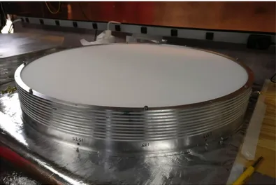
Bicep3 uses alumina ceramic for several of the optical elements. Both lenses and the 50 K IR filter are made of 99.6% pure alumina sourced from CoorsTek1. Moving from the previous-generation HDPE plastic optical elements allow much thinner

(47)

[image:47.612.109.504.80.344.2]

Figure 3.3: Stack of 10 layers of foam filters installed in Bicep3. Each layer is a 1/8" thick HD-30 foam, glued onto aluminum frame with 1/8" spacing. The total filter stack height is 2.5". These filters will be replace for every cryogenic run.

Table 3.4: IR filters installed for Bicep3. The main stack of 10 filters behind the window are listed in order beginning with the closest filter to the window.

2016 Square/pitch 2017

Location Substrate [µm] Substrate

Behind window 3.5 µm Mylar 50/80 HD-30 foam (∼ 290 K) 3.5 µm Mylar 40/55 HD-30 foam 3.5 µm Mylar 50/80 HD-30 foam 3.5 µm Mylar 40/55 HD-30 foam 3.5 µm Mylar 90/150 HD-30 foam 6µm PP/PE 40/55 HD-30 foam 3.5 µm Mylar 50/80 HD-30 foam 3.5 µm Mylar 40/55 HD-30 foam 3.5 µm Mylar 50/80 HD-30 foam 3.5 µm Mylar 90/150 HD-30 foam

(48)

[image:48.612.109.506.69.367.2]

Figure 3.4: AR-coated alumina filter in Bicep3. The alumina filter is coated with a mix of Stycast 1090 and 2850FT. The epoxy is machined to the correct thickness and laser diced to 1 cm squares with avoid differential thermal contraction between alumina and the epoxy.

(2–3 cm instead of 6–10 cm) lens shape for Bicep3’s 580 mm diameter elements, owing to alumina’s higher in-band index of refraction (n=3.1).

(49)

Metal mesh edge filter

Metal mesh low-pass edge filters with a cutoff at 4 cm−1are added to reject out-of-band signal [25]. These filters are made out of multiple randomly orientated metal grid layers, each of them is a thin polypropylene substrate coated with copper film, and hot-pressed fused together to form a shape cut-off edge filter.

The largest filter can be made is smaller than the require size for the Bicep3 focal plane [29]. In order to make sure all detectors are covered and protected, multiple filters are cut to small, 3" by 3" pieces, and they are individually placed directly on top of each detector module, and cooled to 280 mK. Combination of the fabrication process and increase machining on the filter’s edges, we found delamination on the filter in 2016, which degrades the efficiency and shows non-uniform in band spectral response. All the metal-mesh filters are redesigned and replaced prior to 2017 season (Figure 3.5); Fourier Transform Spectroscopy shows the new filter gives a uniform in-band respond (Section 4.1) and increase in optical efficiency measurements indicate functioning filter.

3.2 Cryostat receiver

Cryostat

As shown in Figure 2.2, the Bicep3 cryostat receiver is a compact, concentric-cylinder design, that allows for large optical path while maintaining sub-Kelvin focal plane temperatures [27][30][31]. The outermost aluminum vacuum jacket is around 2.4 m tall along the optical axis and 74 cm in diameter (not including the extension supporting the pulsetube cryocooler). The cryostat weighs around 540 kg fully populated, without attached electronics subsystems. It maintains a high vacuum (∼0.01 mTorr at base temperature) for thermal isolation and is capped at one end by the HDPE plastic window, as described in Section 3.1.

Cryogenic and thermal architecture

(50)

[image:50.612.107.506.67.369.2]

Figure 3.5: Metal-mesh filters mounted on Bicep3 in 2017. The filters are cut to bigger piece, each covering 5 detector modules to minimize the machining required for each filter. Mounting holes are carefully slotted to account for differential thermal contraction. New fabrication process is used for these filters, and each of them are cold tested before installing into Bicep3.

Bicep3 uses a single PT-415 pulsetube cryocooler2, which provides continuous cooling to 35 K at the 1ststage under typical 26 W load and 3.3 K at the 2nd stage under 0.5 W load. A non-continuous, three-stage (He-4/He-3/He-3) helium sorption fridge3 is heat sunk to the nominal 4 K stage and cooled the sub-Kelvin focal plane and supporting structures. The sorption fridge provided continuous sub-Kelvin operation on the focal plane for> 48 and> 80 hours for the 2016 and 2017 season, respectively, with 6 hours of recycling time. These hold time allow us to have a continuous two and three day observation schedule.

The focal plane and ultra-cold (UC) stage (nominal 280 mK) is a planar copper assembly mounted in a vertical stack on two buffer stages (nominal 350 mK and 2 K), each supported and isolated by carbon fiber trusses. The UC stage is comprised

2Cryomech Inc., Syracuse, NY 13211, USA (www.cryomech.com)

(51)

of the 9 mm thick, 46 cm diameter copper focal plane plate that supports the detector modules and a thinner secondary copper plate. The two plates are separated by seven 5 cm tall stainless steel blocks that serve as low-pass thermal filters and dampen thermal fluctuations before reaching the focal plane. Both the focal plane and the secondary UC stage are actively temperature controlled with resistive heaters to 274 mK and 269 mK, respectively. Thermal fluctuations on the focal plane during CMB observation are monitored and controlled by multiple temperature control modules (TCMs). The TCMs include two Germanium NTD thermistors, two heaters, bias and readout circuitry. The JFET readout for the NTDs is located in a readout module mounted to the 4 K baseplate.

Housekeeping

General thermometry uses silicon diode thermometers (Lakeshore4 DT-670) and sub-Kelvin stages are measured with thin-film resistance temperature detectors (Lakeshore Cernox RTDs). Germanium NTD thermistors are mounted directly to the detector tile substrates for more sensitive measurements of the TES thermal bath temperatures, and they are used on both the focal plane and secondary UC stage for the active temperature control input (TCMs). The thermometry, heater, and thermal control signals interface to an external electronics ‘backpack’ mounted directly to the cryostat vacuum jacket that provides biasing, signal pre-amplification, and buffering. A BLASTbus2 ADC system [32] interfaces between the control com-puters and the backpack. Figure 3.6 shows the housekeeping schematic in Bicep3.

RF shielding

Several levels of RF shielding are designed into the 4 K stage and sub-Kelvin structure to prevent RF coupling to the detector signal. Except for the short length of flex ribbon cables that connect the detector modules to the focal plane, all cabling in the cryostat are twisted pair. The ribbon cables are caged by the detector module, copper focal plane module cutout, and the ground plane of the wiring board that accepts the cable. Upon exiting the cryostat, all of the detector signal lines immediately interface with a low-pass filtered connection on the MCE readout electronics box. The 4 K non-optics volume is designed as a Faraday enclosure, with all seams taped, and all cabling passing through additional low-pass filtered connectors. The cage continuously encloses the stack of sub-Kelvin stages by wrapping and sealing a single layer of aluminized mylar between the 4 K stage and

(52)

[image:52.612.116.500.74.347.2]

Figure 3.6: Bicep3 housekeeping schematic.

the edge of the focal plane (Figure 3.10). Finally, the niobium enclosure of each detector module, and detector tile ground plane, enclose the SQUID amplifier/MUX chips.

The cryostat tube acts as a waveguide with microwave frequency cutoff. But the larger diameter in Bicep3 is found to be susceptible to 450 MHz interference from the South Pole station radio system. The interference introduced an azimuth-synchronous signal, as well as transient disturbances to the feed-back based detector readout, and potentially contributed to increased 1/f noise within the science band. Reduced output power and installation of a directional antenna at the main South Pole station emitter in 2017 reduced the radio signal by 35 dB, resulting in the RF signal to be a sub-dominate effect in the science band.

Magnetic shielding

Magnetic shielding is crucial to minimize coupling to the SQUID amplifiers while the telescope scans through the Earth’s field. Cryostat-level shielding is composed of cylindrical, high-permeability Amuneal5 A4K layers, with open ends to avoid

(53)

[image:53.612.249.357.71.394.2]

Figure 3.7: Magnetic shield in Bicep3. The 50 K A4K is highlighted in red (the 300 K vacuum jacket are not shown), as the location of the second-stage SQUID series array (SSA), and the first-stage SQUIDs inside the detector module. The SSA are packaged in niobium boxes and further shielded by Metglas.

interference with the optics and allow data cabling at the bottom. There is one layer on the inner surface of the vacuum jacket spanning the length of the cryostat, and a second, shorter layer on the 4 K stage surrounding the focal plane (Figure 3.7). Laboratory Helmholtz coil measurements of these cylindrical shields in Bicep3 shows a shielding factor of∼30 along the optical axis. The niobium detector module housing provides further shielding of the first-stage SQUID amplifier chips on the sub-Kelvin focal plane, as described in Section 3.3. The second-stage SQUID series arrays on the 4 K stage are packaged in niobium boxes and additionally wrapped with ∼10 layers of Metglas 2714A6. Section 4.6 shows the magnetic shielding performance in Bicep3.

(54)

[image:54.612.108.506.67.371.2]

Figure 3.8: Bicep3 focal plane with 20 tiles.

3.3 Focal Plane

Bicep3 has 2560 detectors, more than a factor of eight greater than a single Keck Arrayreceiver in the same frequency. These detectors are fabricated onto 20 silicon tiles, each housed 128 polarization sensitive transition-edge sensors. We use a modular packaging design of detector tile and readout hardware on the focal plane. It is constructed to provide the necessary thermal stability, magnetic shielding and mechanical alignment to operate the detectors, while at the same time allow us to replace individual tile without affecting the well-performed, existing one.

(55)

[image:55.612.166.448.79.334.2]

Figure 3.9: Sub-Kelvin structure in Bicep3. The bottom ring is connected to the 4 K structure of the receiver. The two middle plate is at 2 K and 350 mK, respectively. The copper structures are thermally connected to the 250 mK stage of the fridge. Each of these temperature stages are thermally isolated by 8 pairs of carbon fiber trusses. 7 stainless steel standoff, are mounted between the two copper plates as an thermal low pass filter.

Sub-Kelvin structure and copper plate

The sub-kelvin structure is mounted on the space above the sorption fridge. It contains three different thermal stages, at 2 K, 350 mK (IC), and 280 mK (UC). Each stages are thermally isolated using 8 pairs of carbon fiber truss structure. Copper heat straps are connected between the sorption fridge to these three stages. All the readout and housekeeping cables are heatsunk onto these stages to reduce the thermal load at the focal plane, which is temperature controlled at 280 mK (Figure 3.9).