Internet traffic dynamics

Munich Personal RePEc Archive

Internet traffic dynamics

Madden, Gary G and Coble-Neal, Grant

Curtin University of Technology, Perth, Australia, Curtin University

of Technology, Perth, Australia

2004

Online at

https://mpra.ub.uni-muenchen.de/10827/

I Introduction

Telecommunications bandwidth has grown at an unprecedented rate in recent years with current esti-mates suggesting that seven percent of the world’s population now has access to the Internet. Indeed, while North America still leads the world in terms of adoption, Table I shows that nearly half of all users now reside outside the Unites States (US). Given the proliferation of telecommunication applications such as Internet browsing, email, Voice over Internet Pro-tocol (VoIP) and video broadband, as well as strong volume growth in the traditional Public Switched Telephone Network (PSTN), it is likely that the growth exhibited in Figure I is likely to continue in the near future. In 1999, for example, standard inter-national telephone traffic grew by over 15 % in 1999 to 107.8 billion minutes. Although VoIP still accounts for only a small fraction of the total voice market, traffic grew tenfold to over 1.7 billion min-utes, with the fastest growth occurring in US-develop-ing country outgoUS-develop-ing routes (TeleGeography, 2001b).

Not surprisingly, such growth has stimulated vigor-ous competition in both national and international telecommunications markets. At the national level, countries such as Germany and Israel have experi-enced spectacular returns to deregulation with long-distance calling market prices dropping 91 % and 94 %, respectively (Newton 2000). Similarly, Tele-Geography (2000) global trends suggest that call vol-ume growth has been stimulated largely by succes-sive price cuts. Technology has played a substantial role, initially by least-cost routing arrangements such as callback and traffic refile, and more recently by routing voice and facsimile transmissions through the Internet, thus providing competitors with the means of reducing or avoiding international settlements.

In response, incumbent carriers have sought to increase their scale so as to defend revenues and deter entry by new competitors. According to TeleGeogra-phy (2001b), submarine cables increased the aggre-gate trans-Atlantic bandwidth by a factor of 12 to

Internet traffic dynamics

G A R Y M A D D E N A N D G R A N T C O B L E - N E A L

Gary Madden is a Professor at CEEM, Curtin University of Technology, Perth, Australia

Grant Coble-Neal is a PhD student

The telecommunications industry has evolved at unprecedented rates with current estimates suggesting that seven percent of the world’s population now has access to the Internet. However, such growth has stimulated vigorous competition in national and international telecommunications markets leading to a price-cost margin squeeze and unsustainable rates of network expansion. This study demonstrates the reliability of established extrapolation methods for forecasting bandwidth demand and provides network managers with the opportunity to observe Internet traffic dynamics. The ability to anticipate periods of peak use and surplus capacity is likely to pay dividends in terms of a more targeted approach to network expansion plans.

Figure I Internet host growth 1981–2001 (Source: Internet Software Consortium, http://www.isc.org/)

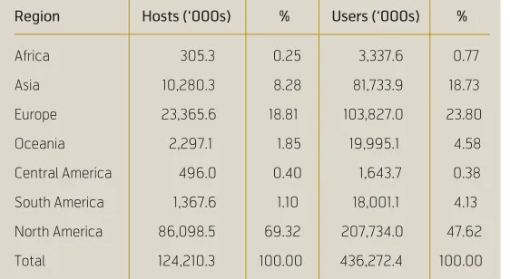
Region Hosts (‘000s) % Users (‘000s) %

Africa 305.3 0.25 3,337.6 0.77 Asia 10,280.3 8.28 81,733.9 18.73 Europe 23,365.6 18.81 103,827.0 23.80 Oceania 2,297.1 1.85 19,995.1 4.58 Central America 496.0 0.40 1,643.7 0.38 South America 1,367.6 1.10 18,001.1 4.13 North America 86,098.5 69.32 207,734.0 47.62 Total 124,210.3 100.00 436,272.4 100.00

Table I Internet hosts and users by region (Source: Telcordia Technologies, http://www.netsizer.com/)

1) _{A terabit is one million million bits.}

-20,000 40,000 60,000 80,000 100,000 120,000

Host nu

mbers (x 1000)

over two terabits per second in just one year.1) Overall, telecommunication’s three basic building blocks, fibre, digital signal processors and routers, are improving their capacity for throughput ten times faster than the mainstream computer industry (New-ton, 2000).2)_{High-speed routers, for example, are} now switching terabits of information each second. In addition, laboratory tests show that a fibre strand the width of a human hair can transmit three trillion bits per second, enough to transmit the entire world’s Internet (Newton 2000).

However, network expansion is expensive. Construc-tion costs can range from USD 4,000 to USD 3 mil-lion per kilometer depending on the choice of upgrade level of dense wavelength-division multi-plexing (TeleGeography, 2001a). Similarly, subma-rine cable installation costs range from USD 0.5 bil-lion for a 10,000 kilometer cable to USD 2.0 bilbil-lion for 30,000 kilometers. Meanwhile, carriers’ main-stream business continues to be cannibalized by the proliferation of Internet Service Providers purchasing flat rate access to upstream network only to offer VoIP to the incumbent carriers’ own customer base.

Thus, while telecommunications traffic continues to grow at a rapid rate, networks are expanding at economically unsustainable rates. Such long-term impacts of technological change are always hard to forecast, but that task is especially difficult in the case of e-commerce, where markets are currently very far from equilibrium. In the ‘land rush’ to secure Internet real estate, to gain first-mover market posi-tion and other advantages, many firms are pursuing strategies that are properly interpreted as the payment of one-time, largely sunk entry costs (Borenstein and Saloner 2001).

In this environment, common carriers will need to develop improved forecast models to accurately pre-dict bandwidth demand and target network expan-sion. This paper uses Internet Traffic Report as a data source that measures Internet bandwidth loads and availability on a continuous basis.3)_{The data is} gen-erated by a test called a “ping”, which measures round-trip travel time along major paths on the Inter-net. Several servers in different areas of the globe perform the same ping at the same time and an index

based on average response times across test servers is calculated.

The traffic index produces a score in the ranges [0, 100]. A zero score is ‘slow’ and 100 is ‘fast’ by com-paring the current response of a ping echo to all pre-vious responses from the same router over the past seven days. Response time in reference to Internet traffic is how long it takes for data to travel from point A to point B and back (round trip). A typical response time on the Internet is 200 milliseconds. To be continually accurate and useful, statistics are gathered at many geographically diverse routers and many geographically diverse ‘satellite’ locations to test from.

This study obtains alternative forecasts of broadband capacity using ARMA, ARARMA, Holt, Holt-D exponential smoothing, Naïve, Robust Trend, as well as a deterministic trend model. The ARMA method is the well-established Box-Jenkins approach to model systematically recurring patterns in stationary data. The ARARMA model, proposed by Parzen (1982), is designed to model long memory processes, using an initial autoregressive specification to filter potentially non-stationary data. Holt’s exponential smoothing fil-ters random noise and extrapolates the underlying lin-ear trend contained in the data while Holt’s-D models time series as a linear trend decaying towards a con-stant. Robust Trend essentially models a time series as a stochastic trend with an outlier filter. Thus, the trend is allowed to adapt as observations accumulate while providing a restrained reaction to sudden unex-pected pulses in the data. Introduced by Grambsch and Stahel (1990), this technique has been shown to perform best for homogenous telecommunications data by Fildes et al. (1998). Naïve is the simple ran-dom walk extrapolation and Trend provides a deter-ministic alternative to Holt, Holt-D and Robust Trend. Both Naïve and Trend are included as indica-tive benchmarks with which to compare forecast accuracy of the alternative methods.

The paper is organised as follows: Section II

describes sample data, and a discussion of the various forecast models is contained in Section III. Model results are presented in Section IV and concluding remarks are presented in Section V.

2) _{A digital signal processor (DSP) is a specialized micro-processor that performs calculations on digitized signals that were originally}

analogue (e.g. voice). DSPs are used extensively for echo cancellation, call progress monitoring, voice processing, and voice and video signal compression. Routers are the central switching offices of the Internet and are the interface devices between different net-work architectures such as x.25, Frame Relay and Asynchronous Transfer Mode. These intelligent devices decide which backbone network to transmit data, monitor the condition of the network and redirect traffic to avoid congestion.

II Data

The data set described and analyzed in this paper is comprised of 59 time-series, each containing 232 observations. These data are sampled from a continu-ous data generating process and sampled daily at 7 AM Australian Eastern Standard Time weekdays for the period February 18, 2000 to March 30, 2001. A representative specimen of these data is shown in Figure II. As described, the data oscillate between zero and 100 and appear to exhibit characteristics typical of stationary series. Another feature, which is common to many of the series in this data set, is the sudden downward spike in the series. These spikes indicate brief periods of unusually high congestion and, depending on the motivation for generating fore-casts, can either be treated as outliers which are atypi-cal of the series or incorporated in the model as an infrequent but important characteristic of the data generating process.

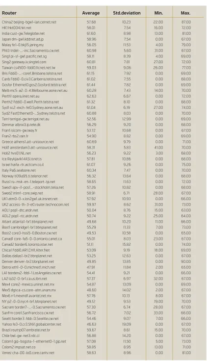
Summary statistics, reported in Table II, highlight the frequency of the downward spikes with 28 of the 59 routers reporting zero minimum values. Regions represented include East Asia, Australia, Western Europe, Israel, Russia, North America and South America. Absent regions include Antarctica, Africa

and most parts of the Middle East. The Denver den-ver-br2.bbnplanet.net router is recorded as providing the fastest response while AOL1 pop1-dtc.atdn.net has the lowest response time. On average, the Perth1 opera.iinet.net.au router provides the consistently fastest response while Yahoo fe3-0.cr3.SNV.global-center.net is typically the slowest.4)

Following Fildes (1992) we analyze the series in terms of frequency of outliers, strength of trend, degree of randomness and seasonality, with the results shown in Figure III through Figure V. An observation (X_t) is classed as an outlier if X_t< L_x– 1.5(U_x– L_x) or X_t> L_x+ 1.5(U_x– L_x), where L_x

denotes the lower quartile and U_xthe upper quartile. The strength of trend is measured by the correlation between the series (with outliers removed) and a time trend, with the absolute value of the trend indicating its strength. Randomness is measured by estimating the regression:

X’_t= α+ βt+ δ₁X’_t-1+ δ₂X’_t-2+ δ_3X’t-3, (1)

where X’_tdenotes the series X_twith outliers removed. The adjusted R2_{is used to measure the variation}

explained by the model. A high R2indicates low

Figure II Japan dm-gw1.kddnet.ad.jp

4) _{Time of day effects and scale of demand may have an impact on router performance. For example, the Perth router services a small}

market and is likely to have relatively low congestion early in the morning, while in real time, the Yahoo router may be at peak demand in the mid-late afternoon.

Time

Tr

affic Index

0 10 30 40 50 60 70 80

18/02/2000 3/03/2000 17/03/2000 31/03/2000 14/04/2000 28/04/2000 12/05/2000 26/05/2000 09/06/2000 23/06/2000 07/07

/2000

21/07

/2000

04/08/2000 18/08/2000 01/09/2000 15/09/2000 29

/09/2000

13

/10/2000

27

/10/2000

10

/11/2000

24

/11/2000

08

/12/2000

22

/12/2000

05

/01/2001

19

/01/2001

02

/02/2001

16

/02/2001

02

/03/2001

16

/03/2001

30

/03/2001

Router Average Std.deviation Min. Max.

China2 beijing-bgw1-lan.cernet.net 57.68 10.23 22.00 87.00 HK1 hkt004.hkt.net 58.01 7.54 16.00 72.00 India cust-gw.Teleglobe.net 61.60 8.98 13.00 81.00 Japan dm-gw1.kddnet.ad.jp 58.96 7.54 0.00 67.00 Malay fe1-0.bkj15.jaring.my 56.05 11.53 4.00 79.00 Phil3 tridel-…-inc.Sacramento.cw.net 60.98 5.60 31.00 67.00 Sing1 pi-s1-gw1.pacific.net.sg 58.11 8.39 4.00 69.00 Sing2 gateway.ix.singtel.com 60.81 7.81 27.00 72.00 Taiwan cs4500-fddi0.ficnet.net.tw 59.03 9.06 26.00 77.00 Bris Fddi0-…-core1.Brisbane.telstra.net 61.15 7.92 0.00 69.00 Canb Fddi0-0.civ3.Canberra.telstra.net 61.02 7.55 0.00 68.00 Gosfor Ethernet0.gos2.Gosford.telstra.net 61.44 7.82 0.00 69.00 Melb mc5-a2-0-4.Melbourne.aone.net.au 60.28 7.43 14.00 70.00 Perth1 opera.iinet.net.au 62.63 6.67 0.00 72.00 Perth2 Fddi0-0.wel1.Perth.telstra.net 61.32 8.10 0.00 68.00 Syd1 sc2-exch-fe0.Sydney.aone.net.au 61.04 6.19 27.00 74.00 Syd2 FastEthernet0-…Sydney.telstra.net 60.88 8.03 0.00 70.00 Terri terrigal-gw.terrigal.net.au 52.56 12.99 0.00 69.00 Denmar albnxi3.ip.tele.dk 56.29 9.20 0.00 68.00 Fran1 isicom-gw.iway.fr 53.72 10.68 0.00 67.00 Fran2 rbs2.rain.fr 54.90 8.82 0.00 69.00 Greece athens1.att-unisource.net 60.69 9.79 0.00 71.00 Holl1 amsterdam3.att-unisource.net 58.31 5.83 41.00 70.00 Holl2 hvs01.NL.net 56.23 9.22 3.00 68.00 Ice Reykjavik14ASI.isnet.is 57.81 10.86 0.00 68.00 Israel haifa-rtr.actcom.co.il 61.07 9.26 0.00 75.00 Italy Pa6.seabone.net 60.34 7.47 0.00 70.00 Norway ti09a95.ti.telenor.net 56.32 13.64 0.00 68.00 Russ1 ru-msk-en-1.teleport-tp.net 58.65 11.63 0.00 72.00 Swed1 apv-i1-pos1…-stockholm.telia.net 57.26 10.82 0.00 68.00 Swed2 mlm1-core.swip.net 58.91 6.71 28.00 67.00 UK1 atm0-0-x.lon2gw1.uk.insnet.net 57.92 10.93 0.00 66.00 UK2 access-th-3-e0.router.technocom.net 59.97 8.62 31.00 73.00 AOL1 pop1-dtc.atdn.net 50.04 8.76 15.00 63.00 AOL2 pop1-rtc.atdn.net 50.74 9.22 25.00 64.00 Atlant atlanta1-br1.bbnplanet.net 49.68 10.20 11.00 66.00 Bost1 cambridge1-br1.bbnplanet.net 55.29 11.33 7.00 73.00 Bost2 core3-hssi5-0.Boston.cw.net 49.53 10.58 0.00 65.00 Canad1 core-fa5-0-0.ontario.canet.ca 55.01 8.03 23.00 67.00 Canad2 border6.toronto.istar.net 51.11 15.82 0.00 74.00 Chica1 Fddi0.AR1.CHI1.Alter.Net 53.09 9.19 18.00 69.00 Dallas dallas1-br2.bbnplanet.net 53.25 12.63 0.00 67.00 Denver denver-br2.bbnplanet.net 49.85 13.85 0.00 90.00 Detroi eth1-0-0.michnet1.mich.net 47.91 11.84 2.00 65.00 LA1 borderx2-fddi-1.LosAngeles.cw.net 54.41 9.21 0.00 66.00 LA2 la32-0-br1.ca.us.ibm.net 57.37 6.97 32.00 67.00 Mex4 core2-mexico.uninet.net.mx 54.87 13.09 0.00 69.00 Mex5 dgsca-cs.core-atm.unam.mx 48.60 14.02 2.00 67.00 Mex6 rr1.mexmdf.avantel.net.mx 57.76 10.13 8.00 67.00 NY p2-0-0.nyc4-br1.bbnplanet.net 49.12 9.53 19.00 70.00 Sacram border7-…-0.Sacramento.cw.net 57.30 6.74 28.00 67.00 SanFrn core1.SanFrancisco.cw.net 56.72 7.02 33.00 66.00 Seattl border3-fddi-0.Seattle.cw.net 54.46 9.07 7.00 66.00 Yahoo fe3-0.cr3.SNV.globalcenter.net 46.63 19.09 0.00 67.00 Brazil routrjo07.embratel.net.br 59.67 8.61 15.00 70.00 Chile bwl-gw-net3.rdc.cl 56.88 14.20 0.00 67.00 Colom1 gip-bogota-1-ethernet0-1.gip.net 57.08 11.50 5.00 73.00 Colom2 impsat.net.co 58.85 8.95 13.00 71.00 Venez cha-00-lo0.core.cantv.net 58.63 8.96 0.00 81.00

randomness while a low R2reveals high randomness. Deterministic seasonality is estimated by regressing the series on an intercept and dummy variables which equal one when t= s, where tdenotes observation

X_t’s position in time and scorresponds to the fre-quency of the seasonality. For example, to test the hypothesis that Mondays are statistically different to bandwidth capacity for the rest of the week, t= {1, 2, 3, 4, 5, …, T}, s= {1, 5, 10, 15, …, T} and dummy variable D_Monday= 1 for t= s, zero otherwise.

Figure III reveals that half the series contain between one and five percent outliers. In percentage terms these data appear slightly more heterogeneous than Fildes’ (1992) telecommunications data. As indicated in the specimen displayed in Figure II, Figure III shows that the data are generally uncorrelated with time. This contrasts with Fildes (1992) where the data there exhibit strong negative trends. Moreover, the histograms in Figure IV and Figure V reveals the

Figure III Outlier frequency Figure IV Strength of linear trend

Figure V Variation explained by linear/AR

Figure VI Daily variation in capacity utilization 0

2 4 6 8 10

0 2 4 6 8 10 12 14 19 Proportion of outlying observation (%)

Fr

eq

u

ency

0 5 10 15 20 25 30 35

-0.4 -0.3 -0.2 -0.1 0 0.1 0.2 0.3 Correlation with time

Fr

eq

u

ency

2 6 10 14 18

-0.02 -0.01 0 0.01 0.02 0.03 0.04 0.05 0.07 Adjusted r squared

Fr

eq

u

ency

No difference Early Week Mid Week Late Week Asia

Australia Europe

North America 0

2 4 6 8 10 12

South America

Asia Australia Europe North America South America

variation in the data presents a high degree of ran-domness with virtually no serial correlation.

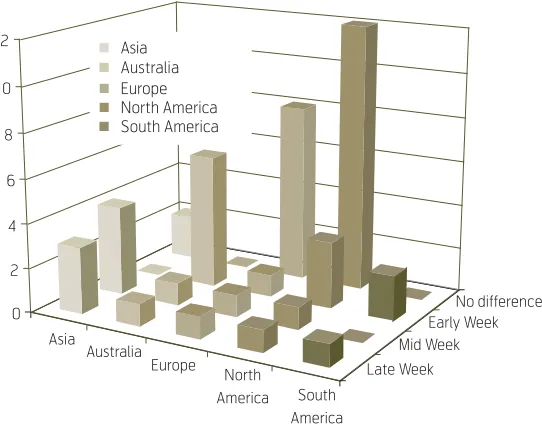
Finally, Figure VI presents some evidence of regular-ity in weekly capacregular-ity variation aggregated by region. As shown, there appear to be regular dips occurring on different days across regions. Asia generally ex-periences lower traffic volumes across the later part of the week, while the majority of Australian routers have excess capacity in the early part of the week. By contrast, Europe and North America experience relatively smooth traffic flows, possibly reflecting more sophisticated capacity pricing regimes and/or advanced network management systems. Finally, variations in South American Internet traffic are tied to specific routers.

5) _{60 day forecasts are necessary due to the existence of standard capacity contracts.}

6) _{Note that ARMA often provides the same accuracy as the Naïve trend forecast. This is due to the general-to-specific modeling}

approach that uses the Akaike Information Criterion to identify the best fitting model from a grid of up to six autoregressive and moving average lags. In many cases, this algorithm identified Naïve as the optimal model.

months with some routers showing surges of up to three months. Given the nature of the index calcu-lations, this possibly reflects the average lagged response time required before routers are expanded to cope with the increased traffic. Once routers are expanded, the Internet traffic index for the router is likely to increase, reflecting the permanently increased capacity.

Overall, the data series exhibit a high degree of ran-domness and regular spikes in index scores. Com-pared to the telecommunications data analyzed in Fildes (1992) and Fildes et al. (1998), these data appear considerably more heterogeneous and less predictable.

III Forecast models and accuracy

measures

Forecast models considered are univariate ARMA, ARARMA, Holt, Holt-D exponential smoothing, Robust Trend, with Naïve and Trend benchmarks. All of these forecast methods have been shown to be reliable by Makridakis et al. (1982), Fildes (1992), Fildes et al. (1998) and Makridakis and Hibon (2000) and consistently perform in the annual M-Competi-tion. Implicit in these analyses however, is that the data are nonstationary, while the data analysed here are believed to be stationary. Given this fundamental difference in assumption some of the forecast tech-niques have been modified to avoid problems associ-ated with over-differencing. For example, the ARMA method is applied rather than ARIMA. ARARMA explicitly questions the practice of differencing to achieve stationarity and has the advantage of utilising information contained in the data normally lost when differencing. Moreover, the approach outlined in Parzen (1982) contains a formal method of determin-ing when it is appropriate to apply the AR filter and hence, the method is adopted intact. Holt and Holt-D methods are techniques for extrapolating the under-lying trend that may be present in the data. Although the deterministic trend correlations are mostly zero, short-run trends may prevail and therefore Holt and Holt-D may be appropriate given their simplicity and reliability. However, to ensure the opportunity for accuracy is maximised, the parameter is optimised (rather than being arbitrarily set once) at each time origin as recommended in Fildes et al. (1998). Robust Trend, however, is modified by not differencing the

data before calculating the stochastic trend. The per-ceived advantage in adopting this method is the out-lier filter and its use of the median rather than mean in the estimator, which may provide some advantage over the simple random walk extrapolation. Thus for direct comparative purposes, Naïve is included as a benchmark model. If the outliers do not bias the esti-mates, the forecasts will be hard to improve on, given the reported properties of the data.

The choice of accuracy measures used in this analysis is guided by the recommendations of Armstrong and Collopy (1992). For the reasons outlined in that paper, the Mean Absolute Percentage Error (MAPE), Median Absolute Percentage Error (MdAPE), % Better, Geometric Mean Relative Absolute Error (GMRAE) and Median Relative Absolute Error (MdRAE) are used. Both GMRAE and MdRAE are Winsorized as recommended by Armstrong and Col-lopy. Mean square error measures are avoided since these statistics are scale dependent and sensitive to outliers.

IV Forecast results

In order to identify forecast methods that perform well four sets of forecasts are created by dividing the data into overlapping time intervals, with each fore-cast method using 114 observations to forefore-cast over the next 60 observations.5)_{In effect, this approach} uses a rolling window beginning at the first observa-tion and steps forward 10 days, re-estimating the forecasts over the next 114 observations. The overall result is 295 forecasts per method with which to judge forecast performance. In evaluating the reliabil-ity of the alternative methods, forecasts are compared with actual values retained in the post-sample data.

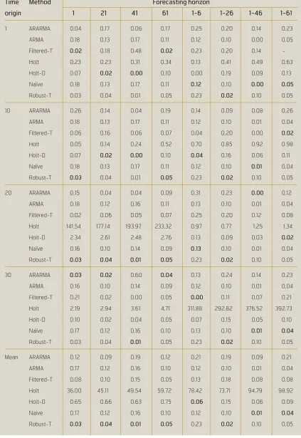
Further evaluation is provided in Table IV, which presents the GMRAE and MdRAE forecast error measures. Both GMRAE and MdRAE compare each method to a no change benchmark forecast for com-parative purposes. Thus, a score less than one

indi-cate the forecast method is at least more reliable than the simplest extrapolation. Using these criteria, it is apparent that both Filtered Trend and Robust Trend consistently outperform the alternatives.

Time Method Forecasting horizon

origin 1 21 41 61 1-6 1-26 1-46 1-61

1 ARARMA 0.04 0.17 0.06 0.17 0.25 0.20 0.14 0.23 ARMA 0.18 0.13 0.17 0.11 0.12 0.10 0.00 0.05 Filtered-T 0.02 0.18 0.48 0.02 0.23 0.20 0.14 -Holt 0.23 0.23 0.31 0.34 0.13 0.41 0.49 0.63 Holt-D 0.07 0.02 0.00 0.10 0.00 0.19 0.09 0.13 Naïve 0.18 0.13 0.17 0.11 0.12 0.10 0.00 0.05

Robust-T 0.03 0.04 0.01 0.05 0.23 0.02 0.10 0.05

10 ARARMA 0.26 0.14 0.04 0.19 0.14 0.09 0.08 0.26 ARMA 0.18 0.13 0.17 0.11 0.12 0.10 0.01 0.04 Filtered-T 0.06 0.16 0.06 0.07 0.04 0.20 0.00 0.02

Holt 0.05 0.14 0.24 0.52 0.70 0.85 0.92 0.98 Holt-D 0.07 0.02 0.00 0.10 0.04 0.16 0.06 0.11 Naïve 0.18 0.13 0.17 0.11 0.12 0.10 0.01 0.04 Robust-T 0.03 0.04 0.01 0.05 0.23 0.02 0.10 0.05

20 ARARMA 0.15 0.04 0.04 0.09 0.31 0.23 0.00 0.12 ARMA 0.18 0.12 0.16 0.11 0.13 0.10 0.01 0.04 Filtered-T 0.02 0.06 0.05 0.07 0.25 0.20 0.12 0.08 Holt 141.54 177.14 193.97 233.32 0.97 0.77 1.25 1.34 Holt-D 2.34 2.61 2.48 2.76 0.13 0.09 0.03 0.02

Naïve 0.16 0.10 0.14 0.09 0.13 0.10 0.01 0.04 Robust-T 0.03 0.04 0.01 0.05 0.23 0.02 0.10 0.05

30 ARARMA 0.03 0.02 0.60 0.04 0.13 0.24 0.14 0.23 ARMA 0.16 0.10 0.14 0.09 0.12 0.10 0.01 0.04 Filtered-T 0.21 0.02 0.00 0.05 0.00 0.11 0.07 0.21 Holt 2.19 2.94 3.61 4.71 311.88 292.82 376.52 392.73 Holt-D 0.10 0.02 0.04 0.05 0.07 0.15 0.05 0.10 Naïve 0.17 0.12 0.16 0.10 0.13 0.10 0.01 0.04

Robust-T 0.03 0.04 0.01 0.05 0.23 0.02 0.10 0.05

Mean ARARMA 0.12 0.09 0.19 0.12 0.21 0.19 0.09 0.21 ARMA 0.17 0.12 0.16 0.10 0.12 0.10 0.01 0.04 Filtered-T 0.08 0.10 0.15 0.05 0.13 0.18 0.08 0.08 Holt 36.00 45.11 49.54 59.72 78.42 73.71 94.79 98.92 Holt-D 0.65 0.66 0.63 0.75 0.06 0.15 0.06 0.09 Naive 0.17 0.12 0.16 0.10 0.12 0.10 0.01 0.04

Robust-T 0.03 0.04 0.01 0.05 0.23 0.02 0.10 0.05

A factor often considered important is the variation in forecast accuracy over the forecast horizon. For example, evidence from M-Competition results indi-cates that some methods are better for short-term forecasts, while others perform best over a longer horizon. Examination of Figure VII, which shows forecast errors for the time period with the least num-ber of outliers, indicates that Holt-D reliably forecast variation in bandwidth capacity for period one through 41, closely followed by Robust Trend. Inter-estingly, ARMA proved most resistant to the distur-bance experienced for periods 46 through 60. A pos-sible explanation for this is the ability of the ARMA method to better model periodic spikes in congestion while both Robust and Filtered Trend provide a muted adaptation to sudden large disturbances.

Figure VIII presents MdRAE statistics calculated across all time origins. This statistic provides a mea-sure that is less susceptible to distortion than the MAPE for series where actual values frequently take zero values. As shown, this measure more clearly dis-tinguishes the performance of the alternatives. Holt-D and Holt (omitted due to substantially larger error measures) are by far the worst performers. By con-trast, ARMA, Filtered and Robust Trend are clustered closely together ranging between 0.5 and one. Not surprisingly, ARMA indicates greater variability with occasional brief spikes above one and below 0.5 while both trend models produce a more consistent estimate. Of interest is the robustness of these meth-ods with little deterioration as the forecast horizon increases.

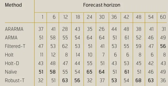
Finally, Table V reveals the proportion of times each forecast performed better than the random walk ex-trapolation across 295 forecasts. Clearly, both Naïve and Robust Trend are the most consistent with the results showing that forecasters can expect these methods to perform better than random walk extrapo-lation 60 % of the time. As a comparison of best to worst, Robust Trend is on average six times more accurate than Holt.

Overall, the results show that bandwidth capacity can be reliably forecast. The MAPE statistics show that Robust Trend tracks the actual index value with aver-age variation of 7.5 % while ARMA is capable of corroborating long horizon forecasts. The inherent stationarity of these data may explain the relative fail-ure of Holt and Holt-D. Both models work best with non-stationary data with a substantial noise-to-signal ratio. Implicit in the implementation of these models is that model parameters are optimized by first- and second-differencing series. The consequence of over-differencing data is the introduction of a unit-root in the error term and estimation of spurious trends.

Figure VII Mean absolute percentage error for time origin 10

Figure VIII Median relative absolute error across all time origins Note: Holt omitted form chart to show detail

Geometric Mean RAE

Method 1 12 24 36 48 60

ARARMA 1.24 1.78 1.87 1.24 1.65 1.54 ARMA 0.99 0.80 0.79 1.00 0.93 1.05 Filtered-T 0.98 0.57 0.75 0.70 0.63 0.77

Holt 4.50 5.39 4.79 6.17 5.76 5.61 Holt-D 1.37 1.23 1.11 1.34 1.23 1.24 Naïve 0.99 0.80 0.79 0.98 0.93 1.05 Robust-T 1.10 0.50 1.13 0.67 0.50 1.00

Median RAE

ARARMA 1.37 2.10 1.92 1.31 2.02 1.53 ARMA 1.00 0.74 0.80 0.99 0.94 1.01 Filtered-T 0.97 0.65 0.87 0.91 0.77 0.83

Holt 7.54 8.19 7.32 8.24 8.20 8.28 Holt-D 2.81 2.88 2.77 3.01 3.14 2.92 Naïve 1.00 0.73 0.81 0.98 0.96 1.01 Robust-T 1.25 0.56 1.17 0.90 0.64 1.08

Table IV Geometric mean RAE and median RAE. Note: Bolded statistic indicates best performing method

0 5 10 15 20 25 30 35

1 6 11 16 21 26 31 36 41 46 51 56 61 Forecast horizon

%

ARARMA ARMA Filtered-T Holt-D Robust-T

0 0.5 1.0 1.5 2.0 2.5 3.0 3.5

Forecast horizon

MdRAE ARARMA

Robust-T

Holt-D Filtered-T Naive ARMA

V Conclusion

Telecommunications bandwidth has grown recently at an unprecedented rate with current estimates sug-gesting that seven percent of the world’s population now has access to the Internet. However, globalisa-tion of the telecommunicaglobalisa-tions industry has led to unsustainable network expansion. In the future, carri-ers will need to develop accurate forecasts as an aid to a carefully targeted approach to expansion plans. This study demonstrates that relatively simple extrap-olation techniques can provide a useful input into explaining broadband traffic movements.

The forecast techniques adopted here are extrapola-tion methods that have performed well in the M-Competition and are easily implemented. This study also highlights the need to better understand data gen-eration characteristics, at least in a broad sense, and suggests that mechanically differencing data without reference to the characteristics exhibited data can yield substantially inferior results. Finally, despite the high degree of randomness and the high fre-quency of outliers, Robust Trend again performed best for telecommunications data.

In general, however, univariate extrapolation tech-niques can at best provide systematic benchmarks on observed data. For more insightful analysis, it is nec-essary to develop structural economic models using price, income data and traffic data. Among the bene-fits of such models are the ability to anticipate cycli-cal fluctuations due to economic factors external to the telecommunications industry, the estimation of price and income elasticities and as a means of deter-mining the degree of reaction and interaction between competitors. The important distinction in adopting this approach is that economic analysis relates to the market for the service that generates these traffic flows. The release of such competitive intelligence would likely provide carriers with substantially great benefits and help to ensure maximal returns to their increasingly scarce investment funds.

References

Armstrong, J S, Collopy, F. Error measures for gener-alizing about forecast methods: Empirical compar-isons. International Journal of Forecasting, 8, 69–80, 1992.

Borenstein, S, Saloner, G. Economics and electronic commerce. Journal of Economic Perspectives, 15, 3–12, 2001.

Fildes, R. The evaluation of extrapolative forecasting methods. International Journal of Forecasting, 8, 81–98, 1992.

Fildes, R, Hibon, M, Makridakis, S, Meade, N. Gen-eralising about univariate forecasting methods: Fur-ther empirical evidence. International Journal of Forecasting, 14, 339–358, 1998.

Grambsch, P, Stahel, W A. Forecasting demand for Special telephone services. International Journal of Forecasting, 6, 53–64, 1990.

Hampel, F R, Ronchetti, E M, Rousseeuw, P J, Sta-hel, W A. Robust Statistics: The Approach Based On Influence Functions. New York, Wiley, 1986.

Makridakis, S, Andersen, A, Carbone, R, Fildes, R, Hibon, M, Lewandowski, R, Newton, J, Parzen, E, Winkler, R. The accuracy of extrapolation (time series) methods; Results of a forecasting competition.

Journal of Forecasting, 1, 111–153, 1982.

Makridakis, S, Hibon, M. The M3-Competition: results, conclusions and implications. International Journal of Forecasting, 16 (4), 451–476, 2000.

Newton, H. Newton’s Telecom Dictionary. New York, CMP Books, 2000.

Parzen, E. ARARMA models for time series analysis and forecasting. Journal of Forecasting, 1, 67–82, 1982.

TeleGeography Inc. TeleGeography 2000: Global Telecommunications Traffic Statistics and Commen-tary. Washington, TeleGeography Inc., 2000.

TeleGeography Inc. (2001a) TeleGeography 2001: Global Telecommunications Traffic Statistics and Commentary. Washington, TeleGeography Inc., 2001.

TeleGeography Inc. (2001b) International

Bandwidth. Washington, TeleGeography Inc., 2001.

Method Forecast horizon

1 6 12 18 24 30 36 42 48 54 60

ARARMA 37 41 28 43 35 26 44 48 38 41 31 ARMA 51 58 55 54 64 64 51 61 52 46 49 Filtered-T 47 53 62 53 51 41 53 55 59 47 56

Holt 11 12 8 14 10 7 6 6 8 6 8 Holt-D 43 48 47 44 55 51 43 53 45 42 43 Naïve 51 58 55 54 65 64 51 61 51 46 49 Robust-T 32 51 63 56 32 37 53 54 68 63 36

Appendix AI Routers by geographic region

Router Location Current index Response time (ms)

Asia

beijing-bgw1-lan.cernet.net China 66 287

hkt004.hkt.net HongKong 61 267

cust-gw.Teleglobe.net India 65 331

tlv-L1.netvision.net.il Israel 66 471 haifa-rtr.actcom.co.il Israel 67 262 hfa-L1.netvision.net.il Israel 61 544

gsr-ote1.kddnet.ad.jp Japan 66 201

doji-alp2-2-1-3-1.mcnet.ad.jp Japan 65 216

POS0-2.oskg2.idc.ad.jp Japan 65 201

fe1-0.bkj15.jaring.my Malaysia 66 263 pi-s1-gw1.pacific.net.sg Singapore 66 334 gateway.ix.singtel.com Singapore 66 285 cs4500-fddi0.ficnet.net.tw Taiwan 66 264 ntt-pc-communications.Tokyo.cw.net Tokyo 66 211

Australia

GigabitEthernet5-1.cha-..brisbane.telstra.net Brisbane 66 418 Pos6-0.woo-core1.Brisbane.telstra.net Brisbane 66 427 Fddi0-0.civ3.Canberra.telstra.net Canberra 64 417 border-gw03-atm301.powertel.net.au Gold Coast 57 373 Ethernet0.gos2.Gosford.telstra.net Gosford 66 397 mc5-a2-0-4.Melbourne.aone.net.au Melbourne 0 0 Pos5-0.exi-core1.Melbourne.telstra.net Melbourne 66 401 So-0-0-1.XR1.MEL1.ALTER.NET Melbourne 64 301

opera.iinet.net.au Perth 63 351

Fddi0-0.wel1.Perth.telstra.net Perth 66 344

c3600.elink.net.au Perth 66 328

sc2-exch-fe0.Sydney.aone.net.au Sydney 65 282 FastEthernet0-0-0.pad8.Sydney.telstra.net Sydney 66 403 So-3-3-1.XR2.SYD2.ALTER.NET Sydney 63 296 FastEthernet0-0-0.pad13.Sydney.telstra.net Sydney 66 400 bb2-gige5-0.rdc1.nsw.excitehome.net.au Sydney 66 261 terrigal-gw.terrigal.net.au Terrigal 64 554

Europe

albnxi3.ip.tele.dk Denmark 67 189

r3-AT2-0-1-Pas5.Hel.FI.KPNQwest.net Finland 67 228

isicom-gw.iway.fr France 64 206

rbs2.rain.fr France 53 239

feth-0-1-0.cr1.Stuttgart.seicom.NET Germany 67 243

athens5.gr.eqip.net Greece 66 264

Pa6.seabone.net Italy 66 255 core1-pos8-0.telehouse.ukcore.bt.net London 66 205 core2-6.csc-1.ldn5.psie.net London 63 190 zcr1-so-1-0-0.Londonlnt.cw.net London 65 185 core1-gig2-0.bletchley.ukcore.bt.net Milton Keynes 65 177 r2-Se0-1-0.0.ledn-KQ1.NL.kpnqwest.net Netherlands 65 209 ti09a95.ti.telenor.net Norway 67 257

cisco0.Moscow.ST.NET Russia 65 241

bgw-ser5-0-0.Moscow.Rostelecom.ru Russia 65 249 apv-i1-pos1-0-0-int-stockholm.telia.net Sweden 66 212

mlm1-core.swip.net Sweden 65 200

atm0-0-x.lon2gw1.uk.insnet.net UK 63 188 access-th-3-e0.router.technocom.net UK 65 180 pos3-0.cr1.lnd5.gbb.uk.uu.net UK 64 180

North America

pos4-1-0-622M.cr1.ANA2.gblx.net Anaheim 66 113

pop1-dtc.atdn.net AOL 65 137

pop1-rtc.atdn.net AOL 65 137

atlanta1-br1.bbnplanet.net Atlanta 66 120 cambridge1-br1.bbnplanet.net Boston 41 178 core3-hssi5-0.Boston.cw.net Boston 0 0 pos1-0-0-155M.ar1.BOS1.gblx.net Boston 65 115 core-fa5-0-0.ontario.canet.ca Canada 66 123 chi-core-03.inet.qwest.net Chicago 66 80 Fddi0.AR1.CHI1.Alter.Net Chicago 65 83 c1-pos2-0.chcgil1.home.net Chicago 66 80 router.mitchell.edu Connecticut 61 138 dallas1-br2.bbnplanet.net Dallas 65 105 dllstx1wcx2-oc48.ipcc.wcg.net Dallas 65 115 denver-br2.bbnplanet.net Denver 64 106 so-1-0-0-3.mp1.Denver1.level3.net Denver 0 0 eth1-0-0.michnet1.mich.net Detroit 53 112 borderx2-fddi-1.LosAngeles.cw.net Los Angeles 64 119 la32-0-br1.ca.us.ibm.net Los Angeles 63 109

mae-west.wenet.net MAE West 0 0

sl-bb21-pen-15-0.sprintlink.net Philadelphia 65 113 pos2-0-622M.cr2.PHI1.gblx.net Philadelphia 66 112 pos1-0-0-155M.ar1.PHI1.gblx.net Philadelphia 66 110 j01-ge-0-1-0-0.phx.opnix.net Phoenix 63 109 p2-1.phnyaz2-cr2.bbnplanet.net Phoenix 65 114 border7-fddi-0.Sacramento.cw.net Sacramento 66 113 core1.SanFrancisco.cw.net San Francisco 66 112 main1-core5-oc12.sjc1.above.net San Jose 65 175 bbr01-p3-0.sntc04.exodus.net Santa Clara 65 113 border3-fddi-0.Seattle.cw.net Seattle 65 113 198.ATM6-0.XR2.SEA1.ALTER.NET Seattle 66 121 pos4-0.core1-ott.bb.attcanada.ca Toronto 63 99 dcr01-g6-0.trnt01.exodus.net Toronto 64 95 299.ATM7-0.XR1.VAN1.ALTER.NET Vancouver 65 124 fa-1-1-0.a04.vinnva01.us.ra.verio.net Virginia 63 109 br1-a3120s8.wswdc.ip.att.net Washington DC 65 113 wdc-core-02.inet.qwest.net Washington DC 65 105 111.at-6-0-0.TR2.DCA6.ALTER.NET Washington DC 63 112 so2-1-0-622M.br1.WDC2.gblx.net Washington DC 66 110 pos2-0-155M.cr1.WDC2.gblx.net Washington DC 67 109

South America

rcorelma1-rcoreats1.impsat.net.ar Argentina 53 321 multicanal-atm1.prima.com.ar Argentina 66 267 gsr01.spo.embratel.net.br Brazil 66 246 fast5-cr2-net5.attla.cl Chile 65 268 telefonica-mundo-chile-no-rev-dns Chile 65 218 gip-bogota-1-ethernet0-1.gip.net Colombia 66 223 cha-00-lo0.core.cantv.net Venezuela 65 190

Gary Madden is a Professor in the Department of Economics and Director of the Communication Economics and Electronic Markets Research Centre (CEEM) at Curtin University of Technology in Perth, Australia. His research is primarily focussed on examining empirical aspects of electronic, information and communica-tions markets. His research funding, which supports CEEM, has come from industry, government and the Australian Research Council. Gary is Editor of the Edward Elgar series, the International Handbook of Telecommunications Economics, Volumes I-III. He is a Member of the Board of Management of the Internatinal Telecommunications Society and a Member of the Editorial Board of the Journal of Media Economics.

email: [email protected]

Grant Coble-Neal was a Research Associate at CEEM, Curtin University from 1999 to 2003. He is currently completing his PhD under Gary Madden’s supervision.