Transient Analysis of Two Dimensional State M/G/1 Queueing Model with Multiple Vacations and Bernoulli Schedule

Transient Analysis of Two-dimensional State M/G/1

Queueing Model with Multiple Vacations and

Bernoulli Schedule

Indra

Associate Professor

Department of Statistics and Operational Research,

Kurukshetra University Kurukshetra, Haryana, 136119, INDIA

Renu

University Research Scholar Department of Statistics and Operational

Research,

Kurukshetra University Kurukshetra, Haryana, 136119, INDIA

ABSTRACT

This paper is concerned with the transient analysis of two-dimensional M/G/1 queueing model with general vacation time based on Bernoulli schedule under multiple vacation policy. As soon as a service gets completed, the server may take a vacation or may continue staying in the system. Whenever no customers are present, after a service completion or a vacation completion, the server always takes a vacation. Laplace transforms of probabilities of exact number of arrivals & departures by a given time t and number of units arrive by time t using supplementary variable technique are obtained. The emphasis in this paper is theoretical but numerical assessment of operational consequences is also given and presented graphically. Finally, some special cases of interest are derived there from.

Key words:

Two-dimensional queueing model;

Multiple Vacation; Bernoulli Schedule; Non-Markovian queue; Supplementary variable technique.

1.

INTRODUCTION

In most of the queueing models, on completion of service to the existing customers, the server stays in the empty system waiting for a new arrival. But there are situations where if the server after completing the service of a customer finds the queue empty, it goes away for a length of time called „vacation‟. This time may be utilized by the server to carry out some additional work. On return from a vacation if it finds one or more customers waiting, it takes them for service on a one-by-one basis until the system empties, after which time it takes another vacation. However, if, on return from a vacation, it finds no customer waiting, then, in the case of single vacation, it remains dormant until at least one customer arrives, whereas in the case of multiple vacation it immediately proceeds for another vacation and continues in this manner until it finds at least one waiting customer upon return from a vacation.

Usefulness of vacation models in queueing theory have been well established as considered being an effective instrument in modelling and analysis of communication networks, manufacturing and production systems. During the last three decades, queueing systems with vacations have been studied extensively. Concerning queueing models with server vacations, Doshi [3] provides excellent survey on vacation models. Takagi [14] also presents the analyses of a variety of queueing systems with vacations. Recently, Tian and Zhang [9,10], provide an updated and comprehensive treatment of various vacation queueing

systems. The queueing models of similar nature have also been reported by a number of authors [1,2,8].

Although the existing results of vacation queues reported in literature are obtained by different methods, but in this paper, based on Bernoulli schedule we consider a single server two-dimensional M/G/1 vacation queue involving only finite sums for the probability that exactly i arrivals and j services occur over a time interval of length t in a queueing system that is idle at the beginning of the interval. Bernoulli vacation schedule was proposed by Keilson and Servi [6]. It is characterized by the feature that if the queue is empty after a service completion then the server becomes inactive and begins a vacation period. If the queue is not empty, then with probability p the server may stay in the system providing service, or with probability (1-p) he may take a vacation of random length.

The advantage of the Bernoulli Schedule is the existence of a control parameter p. And it is shown that the transient state probabilities can be easily computed with recurrence relations. Various aspects of Bernoulli vacation models for single server queueing systems have been studied by Servi[7], Ramaswamy and Servi[13], Doshi[4], and Cooper[12] among several others.

The remainder of this paper is organized as follows. In the next section, we provide a relative formal description of the queueing model and some notations. Section 3 gives definition and difference-differential equations of two-dimensional queueing model. In section 4, we investigate the transient-state solution for the queueing model by using the supplementary variable technique. Section 5 deals with the verification of model and the performance measures and numerical results with their graphical representation are given when the service time is exponential. In section 6, we discuss some special cases. Conclusions are drawn in section 7.

2.

MODEL

DESCRIPTION

AND

NOTATIONS

In this paper, we consider M/G/1 queueing model under following specification. It is assumed that customers arrive according to a poisson process with rate



. Arriving customers form a single waiting line based on the order of their arrivals; that is, they are queued according to the first-come-first-served (FCFS) discipline. The service time is assumed to be generally distributed with probability density function D(x) and

η(x)Δ

is the first order

x 0

η(u)du

D(x) η(x)e

_

probability that the corresponding service time will be completed in time

(x,

x



Δ)

provided the same had not been completed till time x. And

Customers continue to arrive according to a poisson process. We also assume that the server takes a random vacation each time the system is empty. When the server returns from a vacation and finds at least one customer waiting in the system, he begins the service immediately until the system is empty again, otherwise, another vacation is taken and the vacation times are exponentially distributed with parameter w. If the queue is not empty, then with probability p the server may stay in the system providing service, or with probability (1-p) he may take a vacation of random length. We assume that all the considered variables are mutually independent.



 



0 st

dt

f(t)

e

(s)

f

Re(s)0(2.1)

and



1

;

when

i

j

j

i

when

;

0

j

i,

δ





_

1 2

1 2

a,b

n ,n _{n n}

1

N

(s)

(s a) (s b)







(2.2)

The Laplace inverse of

k k k

k

k

m m a t 1

n

m k 1

k 1 1 k p a

i k

Q(p) t e d Q(p)

is (p a )

P(p) (m )!( 1)! dp P(p)

a a for i k

     _      



     Where, n 2 1 m n m 2 m

1

)

(p

a

)

(p

a

)

a

(p

P(p)











1 2 3 n

Q(p) is polynomial of degree mm m   m 1

 _              _                                 1 m,1 2 1 2 m,1 1 2 2 1 n 1 m δ 1 2 m 0 g 2 1 m n 1 1 m bt m n n 1 m δ 1 2 m 0 g 1 1 m n 2 1 m at m n b a, n , n g) (n b) (a 1)! (m m)! (n 1) ( e t g) (n a) (b 1)! (m m)! (n 1) ( e t (t) N (2.3)

3. THE TWO-DIMENSIONAL STATE

MODEL

In contrast to the classical development, we base our analysis of the M/G/1 queue on a model in which the state of the system is given by (i, j), where i is the number of arrivals and j is the number of departures until time t. We

denote the state probabilities for the model as

P

_i,j

(t)

. The solution for

P

_i,j

(t)

provides considerable information

concerning the transient behaviour of the queueing model.

We have



t)Δ (x,

Pi,j,B The probability that there are exactly i arrivals and j departures by time t and the server is busy in relation to the queue and the elapsed

service time lies between x and

x



Δ

, j<i

(t)

Pi,j,V = The probability that there are exactly i arrivals

and j departures by time t and the server is on

vacation, j



i

(t)

P

_i,j = The probability that there are exactly i arrivals

and j departures by time t. j



i

The solution for

P

_i,j

(t)

provides considerable

information concerning the transient behaviour of the queue. The difference-differential equations governing the system are





i,j,B i,j,B i,j,B

i-1,j,B i-1,j

P (x,t) P (x,t) λ η(x) P (x,t)

t x

λP (x,t)(1-δ )

 

    

 

;

i



j



0

(3.1)

i,j,V i,j,V i-1,j,V

j,0 i,j-1,B

0

P

(t)=-(λ+w)P

(t)+λP

(t)+

t

(1-δ )(1-p) η(x)P

(x,t)dx









;

i



j



0

; i≥1 (3.2)

i,i,V i,i,V i,i 1,B i,0

0

P (t) λP (t) η(x) P (x,t) dx (1-δ ) t    _{  } 



;

i



0

(3.3) The appropriate boundary conditions are

i,j,B i,j,V j,0 i,j 1,B

0

P (0,t)Δ wP (t) (1-δ )p η(x)P (x,t)dx





 

_

;

i



j



0

(3.4) Clearly,

i,j i,j,V i,j,B i,j

P (t)=P

(t)+P

(t)(1-δ )

;

i



j



0

(3.5)

Initially, the system starts when there are no units in the system and the server is on vacation, i.e.

P

_0,0,V

(0)



1

,

P

_0,0,B

(0,0)



0

4. SOLUTION OF THE PROBLEM

Using Laplace transforms in above equations (3.1) to (3.4) along with initial conditions and solving recursively, we have

λ

s

1

(s)

P

0,0,V





(4.1) i i,0,V _i

λ

P

(s)=

(s+λ+w) (s+λ)

0

i (4.2)

x 0 i _λ+w,λ i i,0,B i-k+1,1 k=1 k-1 (s+λ+η(u))du 0

P (s)= λ wN (s)

x e dx (k-1)!  





i0 (4.3)

m+1,1

(i-j -m+1-δm+1,1) ,(δm+1,1)

i-j λ+w, λ 1-δ i-j-m i,j,V m=0

j+m, j-1, B 0

P

(s)

λ

(1-p)

N

(s)

η(x)P

(x,s) dx









;

i



j



0

(4.4)

0,h m,0

m,0 x m,0

0

1 i

1-h h i-k

i,j,B

h=0 k=j+1

δ

k-j _λ+w,λ

1-δ k-j-m

i-k+1,δ m=0

(i-k)h+(k-j-m-δ )(1-h) - (s+λ+η(u))du

m,0

(m+j)(1-h)+kh,j-1,B 0

P (s)= w p λ

λ (1-p) N (s)

x

e ((i-k)h+(k-j-m-δ )(1-h))!

η(x)P (x,s)dx



 

 

 

 _

  

 

 

 











0

dx



   

 

 

 



; i>j>0 (4.5)

Taking the Laplace inverse transforms of the above equations (3.6) to (3.10), we have

λt V

0,0,

(t)

e

P



 (4.6)

k i 1 i λt wt

i,0,V i i k

k 0

1

t

1

P

(t)

λ e

e

w

k! w



 

 







_



_







; i>0 (4.7)

t 0 i

i λ+w,λ

i,0,B i-k+1,1

k=1

k-1 (λ+η(u))du

P (t)= λ w N (t)

t

e

(k-1)!

_ 



;i>0 (4.8)

m+1,1

(i-j -m+1-δm+1,1) , (δm+1,1)

i-j

1-δ

i-j-m λ+w, λ i,j,V

m=0

j+m, j-1, B 0

P

(t)

λ

(1-p)

N

(t)

η(x) P

(x,t) dx











;

i



j



0

(4.9)

0,h m+1,1

m+1,1

t m,0

0

1 i

1-h h i-k i,j,B

h=0 k=j+1

δ k-j

1-δ

k-j-m λ+w, λ i-k+1,δ m=0

(i-k)h+(k-j-m-δ )(1-h) - (λ+η(u))du

m,0

(m+j)(1-h)+kh,j-1,B 0

P

(t)=

w p

λ

λ

(1-p)

N

(t)

t

e

((i-k)h+(k-j-m-δ

)(1-h))!

η(x)P

(x,t)dx





_

































; i>j>0 (4.10)

5. PERFORMANCES MEASURES OF

THE SYSTEM

5.1 The Laplace transform

P (s)

i• of the probability

i•

P (t)

that exactly i units arrive by time t is;





i

i i

i i,j,V i,j,B i,j i,j i 1

j 0 j 0

λ P (s) P (s) P (s)(1 δ ) P (s)

(s λ)

 

 

    







;i > 0 (5.1)

And its Inverse Laplace transform is









 

i 0 j

λt i j

i, i

i!

e

t)

(

(t)

P

(t)

P



The Laplace transform of the mean number of the arrivals

is

s λ (s) P i

2 0

i

i, 

     









The arrivals follow a Poisson distribution as the probability of the total number of arrivals is not affected by the vacation times and breakdowns of the server.

Hence, a verification

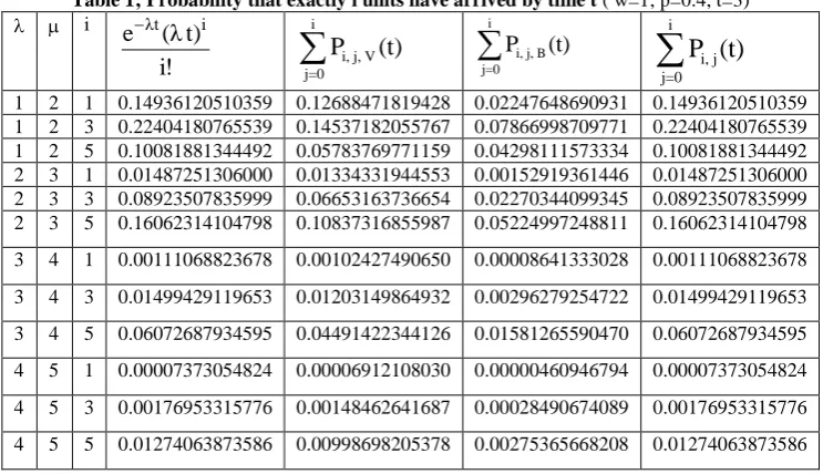
And the numerical results for the probabilities of exact number of arrivals when the server is busy i.e.

i

i, j, B j=0

P

(t)



, when the server is on vacation i.e.

i

i, j, V j=0

P

(t)



,are computed for different sets of

parameter and are summarized in Table–1. Table-1 is based on the relationship (5.1) and its last column shows complete agreement with the Table–1 of Pegden and Rosenshine [11].

5.2 The numerical results for the probabilities that exactly j number of customers have been servedwhen the server is

on vacation i.e. _{i, j, V}

i=j

P

(t)





, when the server is busy i.e.

i, j, B i=j

P

(t)





are computed for different sets of parameters

(

λ 2, μ 3





, w=2, t=2, p=0.4, 0.6, 0.8) and are based

on the relationship _{• j i, j}

i=j

P (t)=

P (t)





where

P (t)

_{i, j} is defined in equation (3.5). By adjusting the value of p, we can control the congestion of the system. And from the numerical results it is obvious that as p increases the probability of departures increases when the server is busy. In figs. 5.1- 5.2, the graphical representation of

_P

_j

_(t)

with the variation of p has been shown.





i

i,j,V i,j,B i,j i 0 j 0

1

P

(s) P

(s)(1 δ )

s



 













i

i,j,V i,j,B i,j i 0 j 0

P

(t) P

(t)(1 δ )

1



 







0 2 4 6 Number of departures(j)

fig. 5.1 0

0.04 0.08 0.12 0.16 0.2

P

ro

b

a

b

il

it

y

o

f

d

e

p

a

rt

u

re

s

w

h

e

n

s

e

rv

e

r

is

o

n

v

a

c

a

ti

o

n

p=0.4 p=0.6 p=0.8

0 1 2 3 4 5

Number of departures (j)

fig. 5.2 0

0.04 0.08 0.12 0.16

P

ro

b

a

b

il

it

y

o

f

d

e

p

a

rt

u

re

s

w

h

e

n

s

e

rv

e

r

is

b

u

s

y

p=0.4 p=0.6 p=0.8

5.3 The probability of exactly n customers in the system at time t, denoted by

P (t)

_n can be expressed in terms

of

P (t)

_{i, j} .

(i) Customers when the server is busy, i.e.

n, B j+n, j, B j=0

P

(t)=

P

(t)





(ii) Customers when the server is on vacation, i.e

n, V j+n, j, V j=0

P

(t)=

P

(t)





And are based on the

relationship _{n j+n, j}

j=0

P (t)=

P

(t)





where

n n, V n, B

P (t)=P

(t)+P

(t)

and

P

_{n, V}

(t)

,

P

_{n, B}

(t)

an

d

P (t)

_n are computed for different values of parameters (

λ 2, μ 3





, w=2, p=0.4). In figs. 5.3 to 5.5, the

graphical representation

of

P

_{n, V}

(t)

,

P

_{n, B}

(t)

and

P (t)

_n with the variation of time t has been shown.

0 1 2 3 4 5 6

Number of Customers(n)

0 0.1 0.2 0.3

P

ro

b

a

b

il

it

y

o

f

n

C

u

s

to

m

e

rs

w

h

e

n

s

e

rv

e

r

is

o

n

v

a

c

ti

o

n

t=1 t=2 t=3 t=4 t=5

Fig. 5.3

0 1 2 3 4 5 6

Number of Customers (n)

0 0.04 0.08 0.12

P

ro

b

a

b

il

it

y

o

f

n

C

u

s

to

m

e

rs

w

h

e

n

s

e

rv

e

r

is

b

u

s

y

t=1 t=2 t=3 t=4 t=5

Fig. 5.4

0 1 2 3 4 5 6

Number of Customers (n)

0 0.1 0.2 0.3 0.4

P

ro

b

a

b

il

it

y

o

f

n

C

u

s

to

m

e

rs

t=1 t=2 t=3 t=4 t=5

Fig. 5.5

5.4 The server‟s utilization time, and the server‟s vacation time i.e. the fraction of time the server is busy & the fraction of time the server is on vacation until time t can also be expressed in terms of

P (t)

_{i, j} .

Thus the server‟s utilization time is

U(t)= i

i, j, B i=0 j=0

P

(t)





. And the server‟s vacation time is

V(t)= i

i, j, V i=0 j=0

P

(t)





.

0 2 4 6 8 10

Vacation Rate (W)

0 0.1 0.2 0.3 0.4 0.5

U

ti

li

z

a

ti

o

n

t

im

e

o

f

th

e

s

e

rv

e

r

100 200 300 400 500 600 700

Vacation Rate(w)

0.3902 0.3904 0.3906 0.3908 0.391 0.3912

V

a

c

a

ti

o

n

t

im

e

o

f

th

e

s

e

rv

e

r

Fig. 5.7

6. SPECIAL CASES

6.1 When there is no Bernoulli schedule, i.e. by substituting p=1 in the difference differential eqns., then above described model reduces to exhaustive service discipline and obtained results coincide with results on Indra [5].

6.2 When the service time is exponential, i.e. by letting η(x) = μ in difference differential equations, we have

m,0

m,0 m,0

i-j

1-δ i-j-m λ+w, λ

i,j,V (i-j-m+1-δ ), (δ ) m=0

(m+j)(1-h)+mh, j-1, B

P (t)= λ μ(1-p) N (t)

* P (t)



; 1 ≤ j ≤ i (6.1)

(t)

N

w

λ

(t)

P

1 -i

0

m m 1, i m, 1

i B

i,0,



  



;i > 0 (6.2)

0,h

m,0

m,0

1 i

1-h h i-k i,j,B

h=0 k=j+1 δ k-j

1-δ k-j-m

m=0 λ+μ,λ+w, λ

(k-j-m+1)(1-h)+(i-k+1)h, i-k+1,δ (m+j)(1-h)+kh,j-1,B

P (t)= μw p λ

λ (1-p)

N (t) P (t)

 

 

 









; 0 < j < i (6.3)

6.3 Along with the case-6.1 & case 6.2, when the server is instantaneously available i.e. no discipline of vacation. Letting

w





in the difference-differential eqns., we have

λt V

0,0,

0,0

(t)

P

(t)

e

P







 





 

  





  

i j λt j i,j i,j,B

K 0

r m

i-k m i k 1 μt

m k

m=0 r 0

μt e i k

λ P (t) P (t)=

μ i! k!

μt 1 m i k !

1 e

r! _{m! j k m ! μt}



   



 

  

 _{ }

 

  _{  } 

   

  _{ } 

  







;i

 

j

0

Then results coincide with eqn. (10) of Pegden and Rosenshine [11].

7. CONCLUSION

The Two-dimensional state M/G/1 queueing system with exponential vacation has been investigated. The numerical analysis clearly demonstrates the meaningful impact of the vacations on the system performances. By adjusting the value of parameter p, we can control the congestion of the system. And utilization time increases and decreases with respect to the increase and decrease in vacation time. Further, with the help of two-dimensional model, we can provide the information on how the system has been operated up until time t. And we have shown numerically as well as analytically that probability of arrivals is not affected by occurrence of vacations.

8. REFERENCES

[1] Alfa,A.S.,(2003), Vacation model in discrete time, Queueing System, Vol.44 (1), pp.5- 30.

[2] Choudhury, G. (2000), An

M

X

/G/1

queueing system with a setup period and a vacation period, „Queueing System,‟ Vol. 36, pp. 23–38.

[3] Doshi,B.T.(1986), Queueing systems with vacations-a survey, queueing sys.,Vol.1, pp.29-66.

[4] Doshi,B.T. (1991), Single server queues with vacations, in: H. Takagi (Ed.), Stochastic Analysis of Computer and Communication Systems, North-Holland, Amsterdam, pp.217–226.

[5] Indra, Some two-state single server queueing models with vacation or latest arrival run, Ph.D. thesis (1994), Kurukshetra University, Kurukshetra.

[6] Keilson J. and Servi, L.D., Dynamics of the M/G/1 vacation model, Operations Research, 35(4), 1987, 575-582.

[7] L.D. Servi, Average delay approximation of M/G/1 cyclic service queue with Bernoulli schedules, IEEE Selected Area of Communication, 4(1986), 813-820. [8] Levy, Y. and Yechiali, U., (1975), Utilization of idle

time in an M/G/1 queueing system, Management Science, Vol. 22, No. 2, pp. 202-211.

[9] NN. Tian and Z.G. Zhang. (2002). “The Discrete-Time GI/Geo/1 Queue with Multiple Vacations.” Queueing Systems, Vol. 40,pp. 283–294.

[10] N. Tian and Z.G. Zhang, Vacation Queueing Models: Theory and Applications,

Springer, New York 2006.

[11]Pegden, C.D. and Rosenshine, M. (1982), Some new results for the M/M/1 queue, Mgt Sc., Vol. 28, 821-828 (1982).

[12]R. B. Cooper, Queues served in Cyclic Order: Waiting Times, The Bell System Tech. J., 49(1970), 399-413.

[13]R. Ramaswami, L.D. Servi, The busy period of the M/G/1 vacation model with a Bernoulli schedule, Stochastic Models, 4(1988), 507-521.

[image:6.595.124.496.98.312.2]

Table 1; Probability that exactly i units have arrived by time t ( w=1; p=0.4, t=3)

  i

i!

t)

(λ

e

λt i i

i, j, V j=0

P

(t)



i i, j, B j=0

P

(t)



i

i, j j=0

P (t)



1 2 1 0.14936120510359 0.12688471819428 0.02247648690931 0.14936120510359 1 2 3 0.22404180765539 0.14537182055767 0.07866998709771 0.22404180765539 1 2 5 0.10081881344492 0.05783769771159 0.04298111573334 0.10081881344492 2 3 1 0.01487251306000 0.01334331944553 0.00152919361446 0.01487251306000 2 3 3 0.08923507835999 0.06653163736654 0.02270344099345 0.08923507835999 2 3 5 0.16062314104798 0.10837316855987 0.05224997248811 0.16062314104798

3 4 1 0.00111068823678 0.00102427490650 0.00008641333028 0.00111068823678

3 4 3 0.01499429119653 0.01203149864932 0.00296279254722 0.01499429119653

3 4 5 0.06072687934595 0.04491422344126 0.01581265590470 0.06072687934595

4 5 1 0.00007373054824 0.00006912108030 0.00000460946794 0.00007373054824

4 5 3 0.00176953315776 0.00148462641687 0.00028490674089 0.00176953315776