4
Design of Stochastic
Simulator for Analyzing the Impact
of Scalability on CPU Scheduling Algorithms
P.K. Suri
HCTM Technical Campus,
Kaithal, Haryana, 136 027, India
Sumit Mittal
M.M. Institute of Computer Technology & Business
Management, M.M. University,
Mullana, Ambala, Haryana, 133 207 India
ABSTRACT
Process scheduling with scalable performance is an issue in computer system. Scalability of scheduling algorithm is its ability to don’t decrease the performance when large processes are under run. The performance of job scheduling policies strongly depends on the properties of the incoming jobs. In this paper, we have analyzed the impact of scalability on different CPU scheduling algorithms with reference to average waiting time, average turnaround time and average response time to determine which algorithm is most suitable for uniprocessor environment. The burst time, arrival time and priority is randomly generated using exponential probability distribution and the performance of all algorithms has been evaluated with reference to arrival time or without arrival time. We use a simulative approach to evaluate the performance and scalability of each algorithm with reference to different number of processes.
Keywords
Uniprocessor environment, Scalability, CPU scheduling algorithms, Simulation.
1. INTRODUCTION
Scheduling refers to a set of policies and mechanisms to control the order of work to be performed by a computer system. Scheduling is the method by which threads, processes or data flows are given access to system resources. The need for a scheduling algorithm arises from the requirement for most modern systems to perform multitasking (execute more than one process at a time) and multiplexing (transmit multiple flows simultaneously). The basic idea is to keep the CPU busy as much as possible by executing a user process or job until it must wait for an event, and then switch to another process. In multiprogramming systems, when there is more than one runable process (i.e., ready), the operating system must decide which one to activate. The decision is made by the part of the operating system called the scheduler, using a scheduling algorithm.
Scheduling, discussions and related project area are very integral design topics, when talking about real-time applications. The CPU scheduling algorithm that is used in the real-time system weighs heavily on the maximization of utilization and throughput, and on the minimization of waiting and turnaround times.
In this paper, some basic following assumptions have been undertaken for the development of simulator:
1. Scheduler allocates the processes to the CPU only when they are stabilized in a steady state;
2. A pool of independent runnable processes is contending for one CPU;
3. The scheduler distributes the resources to the different processes;
4. Uniprocessor environment has been considered for the implementation;
5. There are three scheduling states for each process (ready, running and blocked);
6. Only preemptible and non-preemptible resources are assumed.
7. Simulator is run for n number of processes.
Our stochastic simulator determined the values of waiting time, turnaround time and response time for each job/process. In a similar manner, the average turnaround time, average waiting time and average response time were computed. The processes burst time, arrival time and priority were randomly generated according to negative exponential probability distribution.
1.1 Scheduling Policies
In general, scheduling policies may be pre-emptive or non-pre-emptive.
1.1.1 Non-preemptive Scheduling
In a non-pre-emptive multiprogramming system, the short-term scheduler lets the current process run until it blocks, waiting for an event or a resource or it terminates. The current process releases the CPU either by terminating or by switching to the waiting state.
1.1.2 Preemptive Scheduling
Pre-emptive policies force the currently active process to release the CPU on certain events, such as a clock interrupt, I/O interrupts or a system call. The current process needs to involuntarily release the CPU when a high priority process or job is inserted into the ready queue or once an allocated CPU time has elapsed.
1.2 CPU Scheduling Algorithms
CPU Scheduling is the act of selecting the next process for the CPU to service, once the current process leaves the CPU idle.
1.2.1 First-Come First-Serve (FCFS)
The processes are allocated to the CPU on the basis of their arrival at the queue. Arriving jobs are inserted into the tail (rear) of the ready queue and the process to be executed next is removed from the head (front) of the queue [1], [18]. A long CPU-bound job may dominate the CPU and may force shorter jobs to wait prolonged periods.
1.2.2 Shortest-Job-First (SJF)
The scheduler arranges processes with the least estimated processing time in the queue. The SJF uses the FCFS technique where two processes have the same length next CPU burst [19]. The SJF algorithm may be implemented as either a preemptive or non-preemptive algorithms. Long running jobs may starve, because the CPU has a steady supply of short jobs.
1.2.3 Priority Scheduling (PS)
5 preemption of the current process whenever a higher priority
process arrives. Another variation of the policy adds an aging scheme, where the priority of a process increases as it remains in the ready queue.
1.2.4 Round-Robin Scheduling (RR)
This algorithm is especially designed for time-sharing systems; each process gets a small unit of CPU time. This algorithm will allow the first process in the queue to run until it expires its time, and then run the next process in the queue. In a situation where the process needs more time, the process runs for the full length of the time quantum and then it is preempted and then added to the tail of the queue.
1.3 Scheduling Parameters
The scheduling strategy is good enough with the following possible metrices:
1.3.1 Throughput
It is the number of processes that are completed per unit time. Usually, the goal is to maximize the throughput.
1.3.2 CPU Utilization
Usually, the goal is to maximize the CPU utilization. We want to keep the CPU as busy as possible. Conceptually, CPU utilization can range from 0-100 percent.
1.3.3 Turnaround Time
It is the sum of periods spent waiting to get into memory, waiting in ready queue, executing on the CPU, and doing I/O. Usually, the goal is to minimize the turnaround time.
1.3.4 Waiting Time
This is the amount of time spent in the ready queue to run. Usually, the goal is to minimize the waiting time.
1.3.5 Response Time
It is the time from the submission of a request until first response is produces. Usually, the goal is to minimize the response time.
2. RELATED WORK
Stephen Curran et. al. [10] presented the results of a simulation study comparing scheduling algorithms that schedule independent tasks in multiprocessor versions of UNIX. The results show the difference between the performances of the three algorithms when scheduling a typical UNIX workload running on a small, bus-based, shared memory multiprocessor.
Maria Abur et. al. [13] presented a multiprogramming system which allows more than one process to be loaded into the executable memory at a time and for the loaded process to share the CPU using time-multiplexing. They revealed the simulation of the Scheduling algorithms and comparing their average waiting time to know which has the least average waiting time.
Jochen Krallmann et.al. [20] has done their work on design and evaluation of job scheduling algorithms. They split a scheduling system into three components: scheduling policy, objective function and scheduling algorithm. The main focus is on the selection and evaluation of several scheduling algorithms.
E.O. Oyetunji et.al. [15] has proposed an algorithm which can be used to solve very large classes of the multi-criteria scheduling problems. The revealed that the proposed algorithm performed better than the selected solution methods when the total completion time criterion is much more important than the other criteria.
3. SIMULATION BASED
IMPLEMENTATION
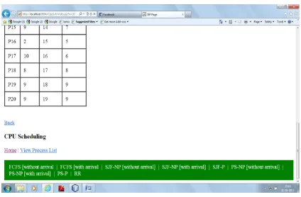
[image:2.595.327.539.259.398.2]In the present study, our objective is to design a stochastic simulator for analyzing the impact of scalability on different CPU scheduling algorithms under uniprocessor environment. Java is used to create the main interface and codes. Once the numbers of processes or jobs are entered, our simulator randomly generated the burst time, arrival time and priority using exponential probability distribution for every process. Then compute the average waiting time, average turnaround time and average response time. In this paper, first we find all the three scheduling parameters for each algorithm without using arrival time of each process and second we find the same parameters with using arrival time of each process. The figure 1 below is the main user interface for the stochastic simulator. This interface is used to run other modules also.
Figure 1 Main user interface for the simulator. The developed simulator determined the average waiting time, average response time and average turnaround time of the different CPU scheduling algorithm. The simulator has been run between (10-500 processes) and than the results is analysed. After considering some of the issues relating to the service pattern of I/O jobs or processes through scheduling goals, it can be concluded that each policy has its own benefits and limitations.
3.1 Analysis of FCFS Algorithm
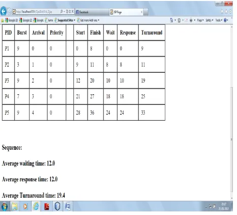
[image:2.595.327.535.611.750.2]Figure 2 shows the analysis of FCFS scheduling algorithm without arrival time and Figure 3 shows the analysis of FCFS scheduling algorithm with arrival time. In these figures, start time, finish time, waiting time, response time and turnaround time with respect to processes are randomly generated using exponential probability distribution. The average waiting time, average response time and average turnaround time with respect to processes are also calculated and shown.
6
Figure 3 FCFS scheduling algorithm with Arrival Time
In the similar manner, the average waiting time, average response time and average turnaround time for all the CPU scheduling algorithms are also calculated which helps a lot in finding the best scheduling policy or analyzing the impact of scalability.
4. RESULTS AND DISCUSSION
The values of average waiting time, average turnaround time and average response time are obtained from the developed simulator for different CPU scheduling algorithms with reference to randomly generated arrival time and without arrival time.
The goal is to minimize the average waiting time and average turnaround time for best scheduling algorithm or to maximize the response time. Table 1 shows the average waiting time of all scheduling algorithms for all the problems sizes in which the arrival time of each job/process is present and Table 2 shows the average waiting time of all scheduling algorithms for all the problems sizes in which the arrival time of each job/process is not present.
Table 1 Average Waiting Time with Arrival Time No. of
Process
FCFS SJF-NP SJF-P PS-NP PS-P RR
10 20 17.7 17.1 21.7 21.7 34
20 32 25.05 21.1 33.45 32.95 37.75
50 105.64 61.12 60.68 93.18 93.24 107.74
100 240.93 142.6 141.87 214.5 214.72 251.65
250 579.06 395.24 395.18 580.02 580.27 693.10
500 1190.82 797.42 795.96 1222.71 1224.01 1376.03
[image:3.595.311.544.77.198.2]The Figure 4 visualizes the impact of scalability on all algorithms with respect to different number of processes verses average waiting time when arrival time is considered.
Figure 4 Shows Average Waiting Time (with arrival time)
Table 2 Average Waiting Time without Arrival Time No. of
Proces
FCFS SJF-NP
SJF-P PS-NP PS-P RR
10 24.5 21 17.1 29 21.7 34
20 41.5 28.95 21.1 40.35 32.95 37.75
50 130.14 80.04 60.68 116.28 93.24 107.74
100 290.43 181.95 141.87 263.99 214.72 251.65
250 703.56 506.88 395.18 704.50 580.27 693.10
500 1440.32 1019.77 795.96 1470.13 1224.01 1376.03
The Figure 5 visualizes the impact of scalability on all algorithms with respect to different number of processes verses average waiting time when arrival time is not considered.
Figure 5 Shows Avg. Waiting Time (without arrival time)
[image:3.595.326.511.235.336.2]Table 3 shows the average turnaround time of all scheduling algorithms for all the problems sizes in which the arrival time of each job/process is present and Table 4 shows the average turnaround time of all scheduling algorithms for all the problems sizes in which the arrival time of each job/process is not present.
Table 3 Average Turnaround Time with Arrival Time No.
of Process
FCFS SJF-NP SJF-P PS-NP PS-P RR
10 30.9 27.4 23.5 35.4 28.1 40.4
20 45.9 33.35 25.5 44.75 37.35 42.15
50 135.22 85.12 65.76 121.36 98.32 112.82
100 295.83 187.35 147.27 269.39 220.12 257.05
250 709.28 512.60 400.90 710.23 586 698.82
[image:3.595.318.539.401.534.2] [image:3.595.57.271.532.686.2] [image:3.595.318.528.636.754.2]7 The Figure 6 visualizes the impact of scalability on all
algorithms with respect to different number of processes verses average turnaround time when arrival time is considered.
Figure 6 Shows Avg. Turnaround Time (with arrival time)
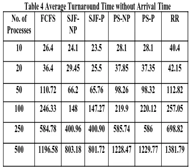
Table 4 Average Turnaround Time without Arrival
Time
No. of
Processes
FCFS
SJF-NP
SJF-P PS-NP
PS-P
RR
10
26.4
24.1
23.5
28.1
28.1
40.4
20
36.4
29.45
25.5
37.85
37.35
42.15
50
110.72
66.2
65.76
98.26
98.32
112.82
100
246.33
148
147.27 219.9
220.12 257.05
250
584.78 400.96 400.90 585.74
586
698.82
500
1196.58 803.18 801.72 1228.47 1229.77 1381.79
The Figure 7 visualizes the impact of scalability on all algorithms with respect to different number of processes verses average turnaround time when arrival time is not considered.
Figure 7 Shows Avg. Turnarond Time (without arrival time)
Table 5 shows the average response time of all scheduling algorithms for all the problems sizes in which the arrival time of each job/process is present and Table 6 shows the average response time of all scheduling algorithms for all the problems sizes in which the arrival time of each job/process is not present.
Table 5 Average Response Time with Arrival Time No. of
Process
FCFS SJF-NP
SJF-P PS-NP PS-P RR
10 20 17.7 16.4 21.7 21.7 16.4 20 32 25.05 17.05 33.45 30.95 27.05 50 105.64 61.12 58.96 93.18 89.76 72.96 100 240.93 142.6 139.24 214.5 214.19 171.68 250 579.06 395.24 395.11 580.02 579.77 442.24 500 1190.82 797.42 792.27 1222.71 1221.03 870.38
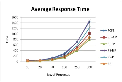
The Figure 8 visualizes the impact of scalability on all algorithms with respect to different number of processes verses average response time when arrival time is considered.
[image:4.595.58.274.119.285.2]Graph 4.5
Figure 5 Shows Avg. Response Time (with arrival time)
[image:4.595.327.526.140.278.2]The Figure 9 visualizes the impact of scalability on all algorithms with respect to different number of processes verses average response time when arrival time is not considered.
Table 6 Average Response Time without Arrival Time No. of
Process
FCFS SJF-NP
SJF-P PS-NP PS-P RR
[image:4.595.72.261.320.485.2] [image:4.595.316.523.329.498.2] [image:4.595.62.272.547.709.2] [image:4.595.327.516.583.723.2]8
Figure 9 Shows Avg. Response Time (without arrival time)
The above shown graph depicts the impact of scalability or the performance of all algorithms with respect to arrival time or without arrival time. It can be observed that as the number of processes increased, waiting time also increased. It is evident that the performances of SJF with respect to all the scheduling parameters are significantly different from the performances of all other FCFS, RR and PS algorithms for all the problem sizes.
5. CONCLUSION
In this work, Four CPU Scheduling Algorithms (FCFS, SJF, PS, and RR) were discussed and measure three scheduling parameters metrics (average waiting time, average response time, average turnaround time) with respect to randomly generated arrival time or without arrival time. In order to know which algorithm gives best performance, we test different jobs sets (10-500 jobs/processes) under uniprocessor environment and shows the impact of scalability on different scheduling algorithms. Here, burst time, priority and arrival time of each process is generated randomly using exponential probability distribution for every algorithm.
Based on the impact of scalability, the shortest job first (SJF) algorithm is recommended for the CPU scheduling problems of minimizing either the average waiting time, average response and average turnaround time.
In future, we design a simulator for the other three variations of Flynn’s Classical Taxonomy of Parallel Processing classification SIMD, MISD, MIMD and also work on the two metrics throughput and CPU utilization of different scheduling algorithms.
Finally, it would be a great challenge to research the scheduling design approaches of trying to schedule soft and hard real-time tasks in the same system
6. REFERENCES
[1] Cooling, J.E, “Software Design for Real-Time Systems, Chapman and Hall, London, UK, 2009.
[2] Stallings, William, “Operating Systems: Internals and Design Principles”, Upper Saddle River, NJ, Prentice Hall, 1998.
[3] Tannenbaum Andrew S and Woodhull Albert S, “Operating Systems: Design and Implementation”, 2nd
Edition, PHI, 2003.
[4] Silberschatz A., P.B.Galvin., “Operating System Concepts”, 6th
Edition, 2001.
[5] Godbole Achuyut S, “Operating Systems: With Case Studies-Unix, Netware, Windows NT”, Tata McGraw Hill, India, 2003.
[6] Banks Jerry, Nicol David M, “Discrete-event System Simulation”, 4th
Edition, PHI, 2005.
[7] Gordan, G., “System Simulation”, 2nd Edition, PHI, Englewood Cliffs, NJ, 2004.
[8] Newell T. James, “Simulation Model to evaluate operational system performance”, in the proceedings of ANSS’81, Annual Symposium on Simulation, March 1981, pp. 103-127.
[9] Schildt Herbert, “The Complete Reference: JAVA” 5th Edition, Tata McGraw-Hill, 2000.
[10] S.W. Curran, “A Simulation Study of Shared-Memory Multiprocessor CPU Scheduling Algorithms”, Computing Systems, University of Toronto, Vol. 3, No. 4, 1990, pp. 551-579.
[11] D.L. Black, "Scheduling support for concurrency and parallelism in the Mach Operating System", IEEE Computer, 23(5), 1990, pp. 35−43.
[12] E.O. Oyetunji and A. E. Oluleye, “Performance Assessment of Some CPU Scheduling Algorithms”, Research Journal of Information Technology 1(1), 2009, Maxwell Scientific Organization, ISSN: 2041-3114, pp. 22-26.
[13] Maria Abur, Aminu Mohammed, Sani Danjuma and Saleh Abdullahi, “Critical Simulation of CPU Scheduling Algorithm using Exponential Distribution” International Journal of Computer Science Issues, Vol. 8, Issue 6, No. 2, ISSN (Online): 1694-0814, November 2011, pp. 201-206.
[14] Charles Crowley, “Operating Systems: A design-Oriented Approach”, Tata McGraw-Hill, New Delhi, 1998.
[15] E.O.Oyetunji and A. E. Oluleye, “General algorithm for solving multi-criteria scheduling problems”, Advanced Materials Research, October 2011.
[16] Savitzky, Stephen, “Real-Time Microprocessor Systems” Van Nostrand Reinhold Company, N.Y, 1985.
[17] M.Kaladevi and Dr.S.Sathiyabama, “A Comparative Study of Scheduling Algorithms for Real Time task”, International Journal of Advances in Science and Technology, Vol. 1, No. 4, 2010.
[18] H.H.S. Lee; “Lecture: CPU Scheduling, School of Electrical and Computer Engineering”, Georgia Institute of Technology.
[19] Yavatkar, R. and K. Lakshman, “A CPU Scheduling Algorithm for Continuous Media Applications”, In Proceedings of the 5th International Workshop on Network and Operating System Support for Digital Audio and Video, 1995, pp: 210-213.
9
7.EDITOR’S PROFILE
Dr. P.K.Suri received his Ph.D degree from Faculty of Engg., Kurukshetra University, Kurukshetra & master’s degree from IIT, Roorkee. Presently, he is working as Dean (R&D) & Chairman (CSE/IT/MCA), HCTM Technical Campus, Kaithal, Haryana, 136 027, India. Prior to joining HCTM, Kaithal, he worked as Professor, Department of Computer Science & Applications and Dean, Sciences & Faculty of Engg., Kurukshetra University, Kurukshetra, Haryana, India. He has supervised thirteen Ph.D.’s in Computer Science and six students are working under his supervision. He has more than 150 publications in International / National Journals and Conferences. He is recipient of 'THE GEORGE OOMAN MEMORIAL PRIZE' for the year 1991-92 and a RESEARCH AWARD–“The Certificate of Merit–2000” for the paper entitled ESMD–An Expert System for Medical Diagnosis
from INSTITUTION OF ENGINEERS, INDIA. His teaching and research activities include Simulation and Modeling, SQA, Software Reliability, Software testing & Software Engineering processes, Temporal Databases, Ad hoc Networks, Grid Computing and Biomechanics.