Surface Roughness Modeling of Titanium Alloy Grinding

(1)

Surface Roughness Modeling Of Titanium Alloy Grinding

Bhola Nath Yadav

1

_{, Vinit Saluja}

2

_{, Mahendra Singh}

3

1_{Research Scholar in Mechanical Engg. Department, Geeta Engg. College, Panipat, Haryana, India} 2_{Asst. Professor in Mechanical Engg. Department, Geeta Engg. College, Panipat, Haryana, India}

3_{Asst. Professor in Mechanical Engg. Department, MIET, Meerut, UP, India}

---*---Abstract -**

Titanium and its alloys have found applications

in aerospace industry, chemical industry, biomedical engineering and marine industries due to high specific strength (strength-to-weight ratio) and excellent corrosion resistance. Despite good mechanical properties grinding of Titanium and its alloys is difficult due to large grinding force, poor heat transfer capability and high chemical reactivity with ambient gases. To assess the effectiveness of titanium grinding, experimental or theoretical evaluation of surface roughness is essential. The experimental methods of surface finish evaluation are costly and time consuming. Hence, a predictive surface roughness model is developed for the grinding of titanium alloy. Which relates the surface roughness values to the process variables, like speed, depth of cut etc. To account for high randomness associated with the process, probabilistic approach is used to predict the surface roughness. The effects of plowing and the elastic deflections on surface roughness are taken into account. Also, the ground surface and grinding wheel profile are simulated using MATLAB, and surface roughness is calculated. The results obtained are then validated by conducting grinding experiments

Key Words: Surface Roughness, Grinding, MATLAB, Surface Roughness Modeling, Chip Thickness ratio.

1.INTRODUCTION

The functional performances of any engineering component depends largely on the properties of the surface as well as the zones immediately under the surface. Different factors that contributes to performance of surface are shape, material properties, residual stresses, surface roughness etc. The overall quality is therefore, dependent upon the final process by which it is produced. Grinding process is usually considered as the final operation in most of the manufacturing processes, due to its ability of producing good surface finish and required dimensional tolerances. Titanium and its alloys have found applications in aerospace industry, chemical industry, biomedical engineering and marine industries due to high specific strength (strength-to-weight ratio) and excellent corrosion resistance. Its density is 60% of that of steel. Amongst all Ti alloys Ti-6Al-4V is the most widely used titanium alloy which is a mixed alpha-beta structure having optimum density, creep strength and fabric ability. Ti is a transition element which changes from alpha (HCP) to beta (FCC) at 883°C. A large no. of surface

roughness models has been developed, which are based upon certain assumptions that may not be valid for actual working conditions. Titanium being a ductile material, is severely affected by the plowing up of material, by the action of grits on to the surface. Hence, the actual value of surface roughness depends largely upon the extent of plowing during the grinding process. Also, there are elastic deflections of the work piece as well as grinding wheel during the grinding process. These deflections will change the effective depth of cut as well as the contact length in grinding contact zone, which will lead to changes in the value of undeformed chip thickness. The surface roughness value is a direct function of undeformed chip thickness, and hence it becomes necessary to consider the effect of these factors while deriving the surface roughness models. Apart from the analytical models, another approach for predicting surface roughness is the development of programming codes in MATLAB for simulating the grinding wheel profile as well as the ground surface. Using these images, we can directly predict the surface roughness values, by giving the kinematic conditions like speed, feed, and depth of cut, material properties etc. as the input variables. The results obtained by the analytical models and the simulations are to be compared with the experimental surface roughness values, by conducting grinding experiments on CNC grinding machine.

2. ANALYTICAL MOEDLING

The analytical model developed in this investigation is to be considered as the early attempt that considers the wheel structure, wheel grit size, work material properties, depth of cut etc. to calculate undeformed chip thickness and the surface roughness. Hence, considering the complex nature of grinding process, the following assumptions have been made:

i. The wheel dressing effect has not been considered in this analysis, and thus the grain distribution with and without dressing is considered to be same.

ii. Analysis is done for no lubrication condition i.e. dry work environment.

iii. The abrasive grits shape is assumed conical. iv. The effect of burn-offs and the effect of rubbing grits

(2)

The number of grains on on the grinding wheel surface in unit length is given by:

Using the number of grits, per unit length, we can calculate number of grits per unit area by following formula:

The values of mean grain diameter and volume fraction of abrasives can be obtained for a specific grinding wheel using following tables:

Table -1: dg max, dg min, and dg mean for different grain sizes [13] Mesh

Size 20 24 30 36 46 54 60 70 80 90 10₀

dg

max(

mm) 0.9

37 0.761 0.587 0.475 0.355 92 0.2 0.256 0.212 0.179 0.151 0.141

dg

min(

mm) 0.7

61 0.587 0.475 0.353 0.292 56 0.2 0.212 0.179 0.151 0.143 0.115

dg

mean(

mm) 0.8

[image:2.595.32.293.280.431.2]

51 0.675 0.531 0.416 0.322 72 0.2 0.234 0.195 0.166 0.146 0.129

Table -2: Volume fraction of abrasive based upon structure no. [13] Structure

number 0 1 2 3 4 5 6 7 8

Abrasive volume fraction

0.68 0.64 0.60 0.58 0.56 0.54 0.52 0.50 0.48

2.2 Distribution Of Grits

The surface profile obtained after grinding consists of grooves left after grinding, and the size of grooves is equal to that of undeformed chip thickness values. Also, the piling up of work material due to plowing action of grits contribute to the surface roughness, thus obtained. Taking into consideration, the random variation of the sizes of individual grits, the undeformed chip thickness values will also be different for different grits, and hence certain probability distribution must be assumed for individual grits. The Rayleigh probability density function can be used to approximate the size of individual grits:

The parameter β, completely defines the Rayleigh PDF, and is a function of material properties, dynamic effects, wheel microstructure etc. The surface roughness values obtained by analytical model will be a direct function of the parameter β. Further, the value of this parameter is known in terms of chip thickness, as per following equations:

The expected value and variance of above equation are given by:

The following figure1 represents the schematic view of grain size distribution in the unit length of wheel surface. On the left, is the curve for Rayleigh distribution.

h

Fig.3.1 Distribution of grits

The magnitude of E(h) can be calculated by Rayleigh probability density function. The better illustration of the grit distribution, in accordance with Rayleigh probability density function can be achieved through following figure:

Fig. 3.2 Rayleigh probability distribution function

2.3 Elastic Deflection

(3)

undeformed chip thickness will be different from that given by empirical formulas:

Fig. 3.3 Elastic deflection model for grits

To calculate the magnitude of these elastic deflection values, kumar and shaw[14] have given separate formulas for local wheel deflection, as well as local work deflection, which are obtained by equating the magnitudes of initial and final lengths of contact zones. The formulas are as follows:

wheel deflection:

And, Local work deflection:

Here, υ is the poisson’s ratio for the grinding wheel. The value of tangential force components can be calculated easily by using a dynamometer, for initial stages. Further, force modeling data can also be used to calculate the force components, under different working conditions. The calculations for l’ i.e. actual contact length are shown in next paragraphs, by considering the thermal effects on the contact length. The total deflection is given by the sum of the local work and local wheel deflections.

3

.4 Calculation for Contact Length

Considering the high energy consumption during the process of grinding, it can be interpreted that a large amount of heat is produced during the process. This heat gets accumulated at wheel-work piece contact zone, and thus raising the local temperature. Due to this increase in temperature, the actual contact length will be much different from that of real contact length. To take into account the thermal effects, Setti et al [13] have derived a formula for actual contact length, by modifying the surface roughness factor in the contact length formula given by Rowe and Qi [8].

Fig.3.4 Chip thickness model The formula is given as follows:

here lg is the geometric contact length given by:

Where ae is the depth of cut. The value of Fn can be calculated easily by using dynamometers. Further, the value of Tm is given by Malkin and Guo[15] as follows:

Where p is the peclet no. and is given by:

θ is known as the thermal diffusivity and can be calculated by formula:

Where, ρ is the density of work piece, and k is the thermal conductivity. The value of c in Malkin’s formula is given by following formula:

Further, for dry condition, heat partition ratio, R can be given by the following equation:

The value of βw is given by the following formula:

(4)

Where M is the mesh size, for a particular grinding wheel

3.6. Surface Roughness Calculation

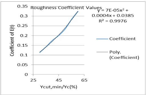
Using different formula’s we found different results The following table shows the value of coefficient for different ycut,min values:

Ycut,min/yc (%) Coefficient of E(Ra)

(for β) Coefficient of E(Ra) (for

E(t))

30 0.1418 0.1132

35 0.1793 0.1431

40 0.2200 0.1756

45 0.2522 0.2012

50 0.2940 0.2346

55 0.3554 0.2836

[image:4.595.35.291.393.560.2]

60 0.4068 0.3246

Table 3 Coefficients of β and E(t) in surface roughness formula

Roughness Coefficient Values

After calculating these coefficients, next step is to calculate the value of undeformed chip thickness. To take into account, the elastic deflections, first we have to calculate grit and work contact deflections, as per equation 2 and 3. For this, values of force components must be calculated. Initially, force values have been measured by conducting experiments, but in actual usage, the force models may be used. The normal and tangential force components at different depth of cuts, as obtained by Kistler dynamometer, for the given grinding parameters are:

S.No. Depth

of Cut Speed ratio Tangential Force Normal Force

1 3 100 2.74 8.04

2 6 100 12.88 37.04

3 9 100 25.41 70.85

4 12 100 32.97 92.2

5 15 100 53.3 129.94

Normal and tangential force components

Through this force components, we can easily calculate the values of actual contact length, as well as the value of elastic deflections. Table 5 represents the values of elastic deflections. The total deflection will be the difference of the two values.

S.N

o. Depth of Cut

Spee d ratio

Wheel deflection (µm)

Workpiece Deflection( µm)

Total Deflecti on(µm)

1 3 100 1.98 0.05 1.93

2 6 100 2.35 0.08 2.27

3 9 100 3.12 0.11 3.01

4 12 100 3.48 0.15 3.33

5 15 100 3.87 0.21 3.66

Wheel and Work piece contact deflections Further, Table 6 represents the value of actual contact length, and the undeformed chip thickness. This chip thickness value takes into account the effect caused by the thermal effects:

S.No. Depth of

Cut Actual Contact Length(mm) Undeformed chip thickness(µm)

1 3 2.842 2.7642

2 6 3.523 4.0371

3 9 4.681 5.1872

4 12 5.263 10.1098

5 15 5.895 11.2859

Actual contact Length and depth of cut

(5)

Variation of chip thickness, actual contact length, and total deflection with depth of cut Hence, after calculating actual chip thickness value, next step is to calculate the value of roughness coefficient from figure 7, for a given depth of cut. Now to relate the value of depth of cut with a particular roughness coefficient, we have to calculate the ratio of critical depth of cut to the actual depth of cut, and then calculating the value of roughness coefficient corresponding to this ratio, by using graph shown in figure 7. The ratio of critical depth of cut to actual, represents the particular value, below which the plowing will takes place, and above which cutting will takes place. The following Table 7 represents the value of depth ratios, and the corresponding roughness coefficients.

After calculating the desired roughness coefficient values, final step is to calculate the value of surface roughness, by using equation 6. The values are shown in Table 8:

S.No. Depth of Cut(µm)

Critical depth of cut(µm)

Ratio

(DOC/CDOC) Roughness Coefficient

1 3 1.42 0.4733 0.2112

2 6 3.23 0.5383 0.2742

3 9 5.25 0.5833 0.3128

4 12 7.15 0.5958 0.3246

5 15 9.52 0.6346 0.3375

Desired Roughness Coefficient Values

After calculating the desired roughness coefficient values, final step is to calculate the value of surface roughness, by using equation 6. The values are shown in Table

S.N

o Depth of cut(µ m)

Undefor med chip thickness

Roughn ess Coeffici ent

Critic al Ratio

Surface Roughness( µm)

1 3 2.7642 0.2112 0.64

33 0.3755

2 6 4.0371 0.2742 0.37

83 0.4223

3 9 5.1872 0.3128 0.33

44 0.5426

4 12 10.1098 0.3246 0.27

75 0.9106

5 15 11.2859 0.3375 0.24

40 0.9294

Predicted Surface Roughness values

Predicted Surface Roughness

The above table shows the values of predictive surface roughness values using the developed analytical model.

3.7 Simulated Wheel Surface

The surface shown below is simulated using MATLAB by approximating the grit distribution to be random in nature. The different regions of the profile are explained in attached chart. The red zones represent cutting grits, which will then be used to plot the ground surface.

(6)

Grit simulation

Cutting Grit Contacting grits Bond Material Plowing Grits

3.8 2D Surface Profile

2D surface profile at 3µm DOC

2D surface profile at 6µm DOC

4: EXPERIMENTAL VALIDATION

The developed analytical surface roughness model and the simulations results has been validated by performing a series of grinding experiments on CHEVALIER SMART H1224 CNC surface grinder. After each experiment, surface roughness has been measured using TALYSURF profile meter. The experiments have been conducted with a conventional C60K5V grinding wheel. The properties of Ti-6Al-4V work piece material used for experimental work are as follows:

Property Value

Density 4.43gm/cc3

Modulus of Elasticity

(W/P) 113GPa

Poisson’s Ratio (W/P) 0.342 Modulus of Elasticity

(Wheel) 25Gpa

Poisson’s Ratio

(Wheel) 0.22

Wheel Dimension 350mm*50mm*127mm

Wheel and Work piece material properties

The grinding experiments are conducted at depth of cut values of 3, 6, 9, 12, 15 µm, and the speed ratio of 100. Before conducting experiments, fine dressing operation has been performed on the wheel with dressing depth of 10 mm, and dressing lead of 10mm/min.

The following table shows the values of the surface roughness values obtained, as well as percentage deviation of the modelled surface roughness value and the simulated surface roughness value from the experimentally calculated value. Further, the bar chart clearly represents the difference between the predicted values and the, experimentally calculated values:

S.No. Dep

th of cut

Analytic al Ra(µm)

Experi mental Ra(µm)

Simulat ed Ra(µm)

Percenta ge Error(An alytical)

Perce ntage error( Simul ation)

1 3 0.3755 0.3056 0.3612 22.87 18.19

2 6 0.4223 0.5302 0.4561 -20.35 -13.98

3 9 0.5426 0.6461 0.7148 -16.02 10.63

4 12 0.9106 0.7653 0.8564 18.98 11.90

5 15 0.9294 0.7876 0.9355 18.00 18.78

Predicted and Experimental results

R

adi

a

l

di

re

cti

(7)

5. CONCLUSIONS

1) An analytical surface roughness model is developed for the grinding of titanium alloys that takes into account the effect of plowing grits as well as the effect of elastic deflections.

2) A MATLAB code is generated, to simulate the wheel surface, and the 2D ground surface, and then surface roughness value is calculated for different depth of cut values.

3) The surface roughness values obtained by the analytical model and the simulations are then validated by conducting grinding experiments on Ti-6Al-4V work piece, using C60K5V grinding wheel.

4) The results obtained are in close correlation with the experimental values, and the average errors of 19.24% and 14.7% are obtained by analytical model and simulations respectively

5.1Scope For Future Work

The effect of rubbing grits and burn-offs on surface roughness can be included, to make the model more accurate.

The grits shape can be more accurately assumed, by taking the contact stylus data, in place of assuming the conical shape of the grits.

While generating the MATLAB code, the trajectory is assumed to be trochoidal in nature, which can be further modified by taking a combination of different curve equations, to make the results more accurate.

REFERENCES

1. S.Y. Liang, R.L. Hecker, Predictive modelling of Surface roughness in grinding, International Journal of Machine Tools and Manufacture, 43(2003) 755-761.

2.M. Sakakura, S. Tsukamoto, T Fujiwara,I. Inasaki, Proceedings of the Institution of Mechanical Engineers, Part B: Journal of Engineering Manufacture 2008 222: 1233.

3.Guoqiang Guo, Zhiqiang Liu, Qinglong an, Ming Chen, Experimental investigation on conventional grinding of Ti-6Al-4V using SiC abrasive, Int J Adv Manufacturing Technology DOI 10.1007/s00170-011-3272-z.

4. J. Hong, J. Jiang, P. Ge, Study on micro-interacting mechanism modeling in grinding process and ground surface roughness prediction, Int J Adv Manuf. Technol.(2012).

5.Z.B. Hou, R. Komanduri, On the mechanics of grinding process- Part I. Stochastic nature of grinding process, International Journal of Machine Tools And Manufacture, 43(2003) 1579-1593.

6. S. Agarwal, P. V. Rao, A probabilistic approach to predict surface roughness in ceramic grinding, International Journal of Machine Tools & Manufacture 45 (2005) 609–616.

7. Albert J. Shih, Jun Qu, Analytical Surface Roughness Parameters of a theoretical profile consisting of elliptical arcs, Machining science and technology Vol. 7, No.2, pp. 281– 294, 2003.

8. W B Rowe, X Chen, Modelling surface roughness improvement in grinding, Part B: Journal of Engineering Manufacture 1999 213: 93.

9. X. Zhou, F. Xi, Modelling and predicting surface roughness of the grinding process, International Journal of Machine Tools & Manufacture 42 (2002) 969–977.

Surface Roughness Modeling of Titanium Alloy Grinding