Airfoil Trailing Edge Noise Generation and Its Surface Pressure Fluctuation

http://dx.doi.org/10.4236/jpee.2015.37003

Airfoil Trailing Edge Noise Generation and

Its Surface Pressure Fluctuation

Wei Jun Zhu, Wen Zhong Shen

Department of Wind Energy, Technical University of Denmark, Lyngby, Denmark Email: wjzh@dtu.dk

Received 26 March 2015; accepted 10 July 2015; published 17 July 2015

Abstract

In the present work, Large Eddy Simulation (LES) of turbulent flows over a NACA 0015 airfoil is performed. The purpose of such numerical study is to relate the aerodynamic surface pressure with the noise generation. The results from LES are validated against detailed surface pressure measurements where the time history pressure data are recorded by the surface pressure micro-phones. After the flow-field is stabilized, the generated noise from the airfoil Trailing Edge (TE) is predicted using the acoustic analogy solver, where the results from LES are the input. It is found that there is a strong relation between TE noise and the aerodynamic pressure. The results of power spectrum density show that the fluctuation of aerodynamic pressure is responsible for noise generation.

Keywords

Large Eddy Simulation, Trailing Edge Noise, Surface Pressure

1. Introduction

As one of the important renewable energy source, wind energy development is growing very fast in recent years. To achieve the ambition of 100% renewable energy in 2050, wind energy is considered as the most important renewable energy source in Denmark. Continuously improving wind energy efficiency has become the major task to keep wind power as an ever growing portion of the world renewable energy. However, among some other problems, public acceptance due to noise from wind turbines becomes a significant barrier for future wind energy development. The issue of wind turbine noise becomes a large factor of uncertainty during wind turbine design and wind farm planning. There is a need of developing wind turbine noise prediction tool that can be used to de-sign low noise wind turbines and silent wind farms.

So far the methods that can be used for wind turbine noise prediction range from the rule of thumb models to advanced Computational Aero-Acoustic methods (CAA). From the simple models to the CAA methods, the computational time grows exponentially. Some of the most widely used methods are summarized below:

 The rule of thumb models.

 Semi-empirical engineering models: BPM [1] [2], NAF Noise [3].

 CAA methods: Acoustic analogy [11] [12], flow/acoustic splitting technique [13]-[15], Direct Numerical Simulation (DNS).

The engineering tools are convenient to provide reasonable good predictions. The CAA methods are able to give physical understanding of the flow induced noise mechanisms. Unless DNS is applied, modelling of turbu-lence cannot be avoided where LES is so far a reliable model for turbulent flow and noise investigations. The aim of the present study is to focus on turbulent flows over an airfoil and its noise generation. By understanding more about the flow characteristics with respect to noise generation, it is possible to design low noise airfoils with special treatment at trailing edge.

2. Numerical Approach

The numerical approach solving the Navier-Stokes equations and the TE noise is presented in this section. Based on the results from LES, the acoustic analogy is performed to calculate noise level at receiver.

2.1. Flow Solver

The Reynolds number of the current study is around 3 million. Although sound propagation is based on com-pressible air, the flow can still be considered as incomcom-pressible because the flow and acoustic solver can be split [13]. The filtered incompressible Navier-Stokes equations, momentum, turbulent stresses and eddy viscosity equations are applied to obtain the turbulent flow data. The filtered incompressible equations are solved by the in-house EllipSys3D code [16] [17]. The code is based on a multi-block/cell-centered finite volume discretiza-tion of the steady/unsteady incompressible Navier-Stokes equadiscretiza-tions in primitive variables (pressure and veloci-ty). The EllipSys3D code is programmed using a multi-block topology, and therefore it is parallelized using a message-passing interface.

(

)

i j ij

i i

2

j i j j

U U τ

U 1 P _ν U

t x ρ x x x

∂ ∂

∂ _{+ = −} ∂ ₊ ∂ ₊

∂ ∂ ∂ ∂ ∂ (1)

2 3

j i

ij t ij

j i

U U

k

x x

τ =ν _∂ +∂ _− δ

∂ ∂

  (2)

(1 ) 2 (1 )

t C k

α α α

ν

ω

(3) 3 3 2 2 1 1 1 1 ( ) ( )

2 j j j 2 j j j

k U U U U

= =

=

∑

∑

The turbulent stresses in Equation (1) is based on the mix model [18] [19] through Equations (2)-(4) where the first filter is identified with an over bar “-” which relates to the finest mesh. The second filter is denoted with a tilde “~” above. The second filter is also denoted as the test filter, it is computed on a mesh twice as coarse as the finest mesh. In Equation (3), ω is vorticity, Δ = (ΔxΔyΔz)1/3 is the reference filter size based on the grid vo-lume. The model constants are C = 0.04 and α = 0.5.

2.2. Acoustic Solver

In this work, the formulation proposed by Farassat [20] is applied. The formulation is the solution of the Ligh-thill’s acoustic analogy [11] with surface sources only when the surface moves at subsonic speed. This formula-tion has been successfully used for helicopter rotor and propeller noise predicformula-tions. At the retarded or emission time, the thickness and loading noise equations are written as

( )

₍

₎

' 0

0

4π ,

1

n

T _f

r _ret v

p t dS

t r M

ρ =   ∂ =_∂  ₋     

∫

x (5)

( )

₍

₎

(

)

'

2

0 0

1 cos cos cos cos

4 ,

1 1

L _{f f}

r _ret r _ret

p p

p t dS dS

c t r M r M

θ θ

π = _∂∂ ₌  ₋  + ₌  ₋ 

   

   

∫

∫

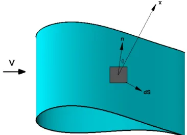
The right hand sides of Equations (5) and (6) are the integrations of time history variables obtained from flow calculations. The variables include wall normal velocity vn, the Mach number of the source in the radiation di-rection Mr, the pressure on the solid wall surface p, the distance between source and receiver r, the angle be-tween the radiation direction and the local wall normal direction θ. Figure 1 shows a sketch of an airfoil where dS indicates one of the typical wall element that is integrated over the entire airfoil surface. It is obvious that the the angle θ will contribute to the noise directivity. The acoustic solver may run in parallel with flow model, in practice the acoustic solver starts when the flow-field is fully established.

3. Results and Discussions

3.1. Brief Description of Surface Pressure Measurements

The wind tunnel used for the surface pressure measurements is optimized for aerodynamic performance. Since TE noise signal is difficult to obtain directly, the surface pressure measurements are performed to evaluate the noise source mechanisms [21]. The measurements are performed for a NACA 0015 airfoil, at a flow speed of 50 m/s, and the airfoil chord is 900 mm. The surface pressure microphones are identified with different numbers and mounted on the airfoil surface. The locations of the microphones are depicted in Figure 2. The microphones are placed along the chord direction, e.g., from leading edge to the trailing edge. They are also spread in the spanwise direction to minimize the flow disturbance due to the upstream microphones. Pressure signals from some of these measurement points (Marked with circles in Figure 2) will be compared with LES results.

Figure 1. Example of an airfoil surface element and the vectors.

3.2. LES Results

A C-type mesh is created for numerical simulation. The mesh is block-structured with 483 grid points in each block. The total number of blocks is 216 which contains a total number of grid points around 24 million. The first wall cell size is in the order of 10−5chord and the ratio of ∆x/∆y is around 25 along the airfoil wall surface. An iso-vorticity plot is shown in Figure 3. At the angle of attack of 4˚, the flow separation is seen on the suction side surface. In Figure 4, the spectral density of the incompressible pressure is compared with measurement da-ta. As seen from the figure, the agreements are found at frequencies below 1000 Hz. The deviation at higher frequencies is due to two reasons: the limited grid size used for LES filter; the wind tunnel fan noise causes high frequency noise, especially the tonal components.

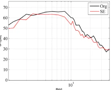
An additional computation is carried out for the same airfoil with a serrated TE. The flow and mesh configu-rations are the same as the previous calculation. As seen from Figure 5, the extended length of the serration (from its root to tip) is 5% of the airfoil chord length and the span of the serration is 10% of the chord. The pressure signals obtained from original airfoil and from the serrated airfoil are compared. In Figure 6, the two signals are selected at x/c = 0.64 and x/c = 0.9. The curves with legend Org1 and SE1 are located at x/c = 0.9. The other two curves are plotted for location x/c = 0.64. As it is seen, the signal closer to TE contains more energy than the one in the upper stream. Also it is observed that near the TE region, the serrated airfoil has less spectral density amplitude which might indicate less noise generation.

3.3. Acoustic Results

The acoustic computation is performed when the turbulent flow is numerically stabilized. The integration of sound source is through Equation (6) where only the loading noise plays the role. The time history data of acoustic pressure is recorded during the simulation. After that, the Sound Pressure Level (SPL) of the original airfoil and the serrated airfoil is compared at a same receiver point which is located at 3-chord distance normal to the suction side of TE. It is interesting to see that the difference of the SPL is quite similar to the one we see in Figure 7. The strength of the incompressible pressure fluctuation at TE has the same behavior as the noise spectra. This indicates that the strength of pressure fluctuation at TE is responsible for noise generation. A small change of TE geometry might influence a lot of noise generation.

Figure 3. Iso-vorticity plot.

Figure 5. Top view of the wall surface mesh with serrated TE.

Figure 6.Spectral density of the incompressible pressure at TE suction side. Comparisons with original airfoil and airfoil with TE serration.

Figure 7. Sound pressure level in 1/3 octave band: comparison with original airfoil and airfoil with TE serration.

4. Conclusion

relatively low angle of attack of 4˚, the computations show that it is the small part of the TE that dominates the noise level.

Acknowledgements

The current numerical study is supported by the European Union’s Seventh Programme for research, technolo- gical developement and demonstration under the grant agreement No 322449. The auther wish to acknowledge the Energy-Technological Development and Demonstration Program under the project (J.nr. 64012-0146) and the Danish Council for Strategic Research under the project (Sags nr. 0603-00506B).

References

[1] Brooks, T.F., Pope, D.S. and Marcolini, M.A. (1989) Airfoil Self-Noise and Prediction. NASA Reference Publication 1218, National Aeronautics and Space Administration, USA.

[2] Zhu, W.J., Heilskov, N., Shen, W.Z. and Sørensen, J.N. (2005) Modeling of Aerodynamically Generated Noise from Wind Turbines. Journal of Solar Energy Engineering, 127, 517-528. http://dx.doi.org/10.1115/1.2035700

[3] Moriarty, P. (2005) NAFNoise User’s Guide. National Renewable Energy Laboratory.

[4] Amiet, R.K. (1975) Acoustic Radiation from an Airfoil in a Turbulent Stream. Journal of Sound and Vibration, 407- 420.

[5] Lowson, M.V. (1993) Assessment and Prediction Model for Wind Turbine Noise: 1. Basic Aerodynamic and Acoustic Models. Flow Soltion Report 93/06, 1-46.

[6] Parchen, R. (1998) Progress Report DRAW: A Prediction Scheme for Trailing-Edge Noise Based on Detailed Boun-dary-Layer Characteritics, TNO Rept. HAGRPT 980023, TNO Institute of Applied Physics, The Netherlands. [7] Bertagnolio, F., Fischer, A. and Zhu, W.J. (2013) Tuning of Turbulent Boundary Layer Anisotropy for Improved

Sur-face Pressure and Trailing-Edge Noise Modeling. Journal of Sound and Vibration, 333, 991-1010.

[8] Wolf, A., Lutz, T., Würz, W., Krämer, E., Stalnov, O., Seifert, A., et al. (2014) Trailing Edge Noise Reduction of Wind Turbine Blades by Active Flow Control. Journal of Wind Energy. http://dx.doi.org/10.1002/we.1737

[9] Howe, M.S. (1978) A Review of the Theory of Trailing Edge Noise. Journal of Sound and Vibration, 61, 437-465.

http://dx.doi.org/10.1016/0022-460X(78)90391-7

[10] Howe, M.S. (1991) Noise Produced by a Sawtooth Trailing Edge. Journal of the Acoustic Society of America, 90, 482- 487. http://dx.doi.org/10.1121/1.401273

[11] Lighthill, M.J. (1952) On Sound Generated Aerodynamically. I. General Theory. Proceedings of the Royal Society of

London A, 211. http://dx.doi.org/10.1098/rspa.1952.0060

[12] Ffowcs Williams, J.E. and Hawkings, D.L. (1969) Sound Generated by Turbulence and Surfaces in Arbitrary Motion.

Philosophical Transactions of the Royal Society, A264, 321-342.

[13] Hardin, J.C. and Pope, D.S. (1994) An Acoustic/Viscous Splitting Technique for Computational Aeroacoustics.

Theo-retical and Computational Fluid Dynamics, 6, 321-342. http://dx.doi.org/10.1007/BF00311844

[14] Shen, W.Z. and Sørensen, J.N. (1999) Comment on the Aeroacoustic Formulation of Hardin and Pope. AIAA Journal,

1, 141-143. http://dx.doi.org/10.2514/2.682

[15] Zhu, W.J., Shen, W.Z. and Sørensen, J.N. (2011) High-Order Numerical Simulations of Flow Induced Noise.

Interna-tional Journal for Numerical Methods in Fluids, 66, 17-37. http://dx.doi.org/10.1002/fld.2241

[16] Michelsen, J.A. (1992) Basis 3D—A Platform for Development of Multiblock PDE Solvers. Technical Report, AFM 92-05, Technical University of Denmark, Denmark.

[17] Sørensen, N.N. (1995) General Purpose Flow Solver Applied to Flow over Hills. Risø-R-827-(EN), Risø National La-boratory, Roskilde, Denmark.

[18] Ta Phuoc, L. (1994) Modèles de Sous Maille Appliqués aux Ecoulements Instationnaires Décollés. Proceedings of the

DRET Conference: Aérodynamique Instationnaire Turbulente-Aspects Numériques et Expérimentaux, Paris, France:

DGA/DRET Editors.

[19] Sagaut, P. (2006) Large Eddy Simulation for Incompressible Flows. 3rd Edition, Springer. [20] Farassat, F. (2007) Derivation of Formulations 1 and 1A of Farassat NASA/TM-2007-214853.