Advanced Cost based Graph Clustering Algorithm for Random Geometric Graphs

Advanced Cost based Graph Clustering Algorithm for

Random Geometric Graphs

Mousumi Dhara

Research Scholar

Department of Computer Engineering, IIT (BHU)

K. K. Shukla

Professor

Department of Computer Engineering, IIT (BHU)

ABSTRACT

There is an increasing interest in the research of clustering or finding communities in complex networks. Graph clustering and graph partitioning algorithms have been applied to this problem. Several graph clustering methods are come into the field but problem lies in the model espoused by the state-of-the-art graph clustering algorithms for solving real-world situation. In this work, an attempt is made to provide an advanced cost based graph clustering algorithm based on stochastic local search. The proposed algorithm delivers significant improvement in robustness and quality of clustering in case of real-world complex network problems. The approach is to compute the cost (scaled cost) accurately when a target node is moved from source to destination cluster. The accurate cost is obtained by computing the induced effect which is evaluated by considering the relevance of nodes related to both source and destination clusters other than the target node during clustering. In our algorithm, moves are only made if the target node has neighbouring nodes in the destination cluster (moves to an empty cluster are the only exception to this instruction). Another important attachment in our approach is in inclusion of the aspiration criteria for the best move (lower-cost changes) selection when the best non-tabu move contributes much higher cost compared to a tabued move then the tabued move is acceptable otherwise the best non-tabu move is approved. Extensive experimentation with synthetic and real random geometric graph (RGG) benchmark datasets show that our algorithm outperforms state-of-the-art graph clustering techniques on the basis of cost of clustering, cluster size, normalized mutual information (NMI) and modularity index of clustering results.

General Terms

General Terms: Graph clustering, Data mining et. al.

Keywords

RGG, Cost of clustering, Cluster size, Normalized mutual information (NMI) and Modularity index of clustering results

1.

INTRODUCTION

There is an extensive approach to the analysis of complex social and economic phenomena in assembling the participating individuals or objects and their interactions into a network (nodes and links) and to deduce functional characteristics of the entire system from this static web of connections [1–5]. In the real world scenario, many complex systems exist in the form of networks, such as social networks

[6], biological networks [7,8], Web networks [9-11], collaboration networks [12-14], neural networks [15], food webs [16,17], and the citation network of scholarly papers [18], which are communally referred to as complex networks. One of the major goals in various applications of these networks is to measure and understand the characteristic properties and behaviour of these networks under various processes taking place in the networks.

Over the last decade, several widely studied large-scale properties of real-world networks have been revealed, e.g. the broad (scale-free) distribution of node degree [19], overrepresented small subgraphs [20,21] and various signatures of hierarchical or modular organisation [22]. Also, various suitable measures have been defined to quantify the importance of the individual nodes in the networks. If a vertex lies on many shortest paths running between other vertices, it plays a central role in information flows Ref. [23] and is accountable for the vulnerability of the system.

real-life systems they model and permit for the design of efficient algorithms. RGGs have been used sporadically in real networks modelling [41] and widely in continuum percolation [42, 43], but almost exclusively in two and three dimensions. Recently, continuum percolation has been used in the study of the stretched exponential decay of the correlation function in random walks on fractals and the conjectured relation to relaxation in complex systems [44]. However, continuous systems in general and RGGs in particular are relevant whenever we need a multidimensional system with a metric, as for example when modelling the spread of diseases [45]. Although the origin of random geometric graphs can be traced back to the work of Gilbert in 1961 [27], they were not theoretically analyzed until recent years.

To achieve some meaningful information about the network models and to visualize the details of the networks with many applications in a number of disciplines, clustering is necessary and it is more fruitful job than other ones. Graph clustering algorithms emphasis on clustering the nodes of a graph [46], [47]. It can expect from a graph clustering scenario that it contains a collection of sub graphs (nearly completely connected) and a small fraction of edges are existed between them for interconnection.

Recently, spectral clustering is getting immense popularity because of the convention of eigenvectors applied in various machine learning tasks [48]. In the recent past, various other graph clustering algorithms came into the field like restricted neighbourhood search clustering (RNSC) [49], Markov clustering (MCL) [50], super paramagnetic clustering (SPC), Genetic Algorithm, Molecular Complex Detection (MCODE), Local Clique Merging Algorithm (LCMA), etc.

RNSC, which is a cost based clustering method and performs local search iteratively to obtain optimum clustering in an efficient way. RNSC is a stochastic technique which uses restricted neighbourhood search concept. It also acts like a metaheuristic technique like tabu search, described in [51] and also can be used in various search space schematics. Tabu search concept was first proposed by Glover in [51] and is described in detail in [51]. The idea behind it is to allow cost-based local search algorithms to enter, then leave local minima by preventing the search from retracing its steps and

settling in a local minimum. RNSC is also known as Variable neighbourhood search [52]. The main goal of this algorithm is to find the best cost clusterings (lower cost) from the set of clusterings of a graph by assigning some cost functions (Naive cost function and scaled cost function). The memory requirement for RNSC is O (n^2). The complexity of a move in the naive cost function is O (n), which is the size of the restricted neighbourhood of a move M.

MCL is an efficient clustering method in weighted graphs, based on the prototype of stochastic flow simulation technique. In this technique, clusters (a natural grouping of densely flow-connected vertices) are obtained by using two operators: flow expansion and inflation. MCL technique performs well for sparse graphs. The expansion step of MCL has complexity O (n^3), assuming some small bound on the expansion exponents ei. The inflation has complexity O (n^2).

In this paper, we present an advanced or accurate cost based graph clustering algorithm that improves some objectives related to graph clustering by focusing the drawbacks of RNSC’s cost evaluation and clustering approach. Basically, the accuracy in cost measurement is established by mathematical observation of the network structure during clustering. Performance evaluation of the proposed technique is prepared using synthetic and real random geometric graph benchmark dataset. The widespread experiments on these datasets demonstrate that the proposed technique is producing better clustering effectively in terms of robustness and optimality.

2. BACKGROUND

RNSC [49] is a local search meta-heuristic technique which is used to minimize the cost of clustering in the solution space. According to Stijn van Dongen, the vertex-wise performance criteria for clustering of unweighted graphs as the sum of the coverage measure taken on each vertex. In RNSC, a simple integer-valued cost function (called the naive cost function) is used as a pre-processor to produce initial clustering results on a graph and after that to evaluate the low-cost clustering result, a more expressive (but less efficient) real-valued cost function (called the scaled cost function) is applied. The scaled function tries to optimize the output from naive function and reach to the global optimal solution. For a clustering C on an un-weighted graph G (V, E) in which |V| = n, more expressive scaled coverage measure is in the following expression where, N (v) is the open neighbourhood of v.

1 0

( , , )

( , , )

( , , )

1

( )

out in

v

G C v

G C v

Cov G C v

N v C



 

 

(1)

The scaled cost function is expressed as in Eq. (2).

1 0

1

1

( , )

(

( , , )

( , , ))

3

| ( )

|

s out in

v V v

n

C G C

G C v

G C v

N v

C









 





(2)

[image:2.595.56.280.229.437.2]

Cost functions for weighted graphs: If Wu, v is the weight of the edge between vertices u and v. αv is the cost numerator for v in a simple unweighted graph and that can be transformed to

achieve



_v, the cost numerator for v in a weighted graph. Define



_v as follows.

,

(1

,

).

v v

v u v u v

u C u C

w

w



 











(3)

|

( )

|

v v

v V

N v

C











(4) With the new cost numerator



_v defined in Eq. (4), the

scaled cost function may be written as in Eq. (5).

1

( , )

3

v s

v V v

n

C G C













(5)

3. Description of Advanced Cost Based

Graph Clustering algorithm (ACOGCT)

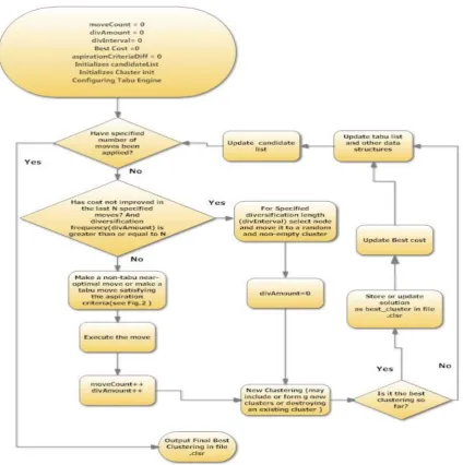
The proposed algorithm is developed by using advantage of the intellectual conception of tabu search. The main intension is to design a more significant and optimal algorithm for providing better clustering results by exploring some advanced concepts as aspiration criteria in tabu search. The step by step evaluation of our algorithm is deliberated below. In this section, summary of the steps of the developed algorithm is presented to acquire a quick insight into the logic involved.

Step 1

Create an initial clustering solution: This step involves assigning nodes to their cluster either on a random or on some other basis.

Step 2

Generate Move list: Generate a set of all possible moves and associate cost with them.

Step 3

Update Move list: Update the list of moves based on the last move. Last move may have brought changes in the cost of nodes in the move’s source or destination cluster or both. They might be inclusion or exclusion of the moves.

Step 4

Move selection: Move may belong from the candidate list or be a diversification move.

Step 5

Apply the move: Update cluster and nodes about the application of the move. Save the best answer at local minima.

Step 6

Check: If the specified number of moves has not been applied, then jump to update move list. Step 7

Return: Print the best answer and Exit.

3.2 Comparative features of RNSC and

proposed algorithm

The proposed algorithm is the refinement of RNSC with respect to few positive aspects. These features are conferred with proper explanations.

3.2.1 Key positive features

Few positive features are pointed out here to lay the foundation of the algorithm better compare to RNSC.

 Scale cost evaluation is O (n) in RNSC. This can easily be done in O (1) time if the information about current node, and its cluster contribution are pre-computed.

 RNSC might tabu some very good moves based on the tabu criteria. Instead, in the proposed algorithm, aspiration criteria serve the sole purpose of avoiding tabu (based on the relative cost of the best non-tabu move).

 Regeneration of all possible moves to select the best move, each time before it is applied in RNSC.

 Moves are considered only if the target node has neighbouring nodes in the destination cluster (moves to empty cluster are the only exception to this rule).

 The effect of a move for any cost scheme considered in RNSC is not exact in nature. They ignore the effect of moving on nodes other than the target node.

 Cost scheme is evaluated in RNSC on an absolute basis after each move. Instead, in the proposed algorithm, costs are evaluated relative to starting clustering state and iteratively. The cost of the starting cluster is set equal to zero and effects of moves are added upon it. So, the effects of a move are added to get the cost of current clustering state relative to the initial clustering solution.

3.2.2 Features retained in our proposed algorithm

The properties that are kept unchanged and taking advantage of this retained properties of RNSC is focused here.

 Short-term memory considerations using Tabu criteria are actively used.

 As in the case of RNSC, diversification moves are applied when in the recent past no good solution was found.

 Scale cost scheme forms the basis for evaluating the cost of a move.

3.3

Greedily create an initial clustering

solution

The initial clustering solution technique is explained here with the proper manner:

I. Select the node with the highest degree with no cluster assigned yet.

II. Add node to a new cluster and its unassigned neighbours are also put into the same cluster. III. If all nodes haven’t been assigned yet then go

back to the initial step I.

3.4 Move selection

The idea behind the selection of a move similar to the technique used in RNSC, where type of move is decided based on the previous clustering costs or improvements. Diversification move is executed when there has been no improvement in the best cost of the clustering over the last specified interval of time otherwise a normal move (in our case tabu move) is applied. Diversification when run shuffles the current clustering by the specified amount of diversification period and frequency, even if it means a significant increase in the current cost. This helps us to get out of any local minima where we might have been stuck in and explore some new possible clusterings.

If there is no need for diversification, best move from the candidate list is selected if it’s not on the tabu list (i.e. the target node wasn’t moved in the near past).

Our algorithm satisfies the aspiration criteria, whereas RNSC does not follow this criterion. Aspiration criteria allow selection of a move even if it’s already tabued when the best non-tabu move incurs a cost which is much higher than itself. The basic idea is that, if the best move is already tabued instead of ignoring it, check the feasibility see if this move is going to be much better than the best non-tabu move existent. This difference between best move cost (which is in tabu) and best non-tabu move cost, if less than the aspiration level, then select the non-tabu move, otherwise select the best move.

3.5 Application of a MOVE

In this algorithm when a move is made then the target node is removed from the source cluster and added to the destination cluster. During execution of a move, a list of changes that contains the whole information about the source and target cluster is passed to each node related to those sources and destination cluster. Each node now quickly updates based on the changes it's going to incur the value for the total edge connections and edge weight with the neighbouring nodes in the cluster. These values later help in O (1) scale cost associated with the node.

After the updates on nodes and clusters performed tabu-list is informed about the changes that have occurred. Tabu list now identifies the last target node as tabu with duration depending on the previous tabu duration value associated with the target node. Greater the previous tabu duration value much greater will be the penalty added to the target node, so that the occurrence of moves with the node is forbidden.

3.6 Adaptive Scaled Cost Estimation

Move stored in the candidate list other than consisting of a target node to be moved from the source cluster to destination cluster and also the recomputed cost is going to incur. The scaled cost scheme for weighted graph is described briefly in this section.

The scaled cost scheme: RNSC’s scaled cost evaluation is costly due to the O (n) computation of a denominator value ( ). In RNSC only the direct cost associated with the move is considered i.e. the changes in the cost for target node. It does not consider the effect induced on the nodes of the source and destination cluster.

In our algorithm, only the scaled cost evaluation is used. Scaled cost evaluated with any node could be computed in O (1) time against the O (n) time spent in the case of RNSC. The faster computations are due to constant update about the changes in the cluster to its node. Each node now quickly updates based on the changes it's going to incur the value for the total edge connections and edge weight with the neighbouring nodes in the cluster. The value of the total number of edge connections and total edge weights with the neighbouring nodes in the cluster have incurred during the node update process and based on that incurred value some changes are made for each node. This argument justifies that there is no need of using the naïve cost scheme. A cost change caused by the move is due to the sum of changes in the cost associated with the nodes of the source and the destination cluster. Direct cost is the change in the cost of a target node (moving node) itself. Induced cost is the sum of changes in cost of nodes belonging to the source or destination cluster other than the target node.

3.6.1 Logical view of cost changes with move

Evaluations

In the new algorithm, only scale cost scheme from RNSC is used for move evaluations. Scale cost evaluations have been simplified to simple constant time operations, due to active update of information corresponding to nodes about its cluster contributions. Further, move evaluations have been broken down and simplified for a clearer understanding.

Let scale cost for node “t” in a cluster “c” is represented by Scale cost (t, c). For a graph with n vertices, Scale cost (t, c) ignores the constant multiplier of (n-1) /3 during the discussion ahead. Scale cost value combines results of contributions from interconnection, intra-connection and neighbourhood (nodes present in the cluster c or have an edge with the node n).

α (numerator) = Weight due to inter-cluster connections of t+ weight due to intra-cluster connections of t.

β (denominator) = neighbourhood size.

Scale Cost= α/β (6) Inter-Cluster contributions are the sum of all the connections from “t” to nodes in clusters other than “c”. This adds the cost associated with inter-cluster connection, as they should have formed an intra-cluster connection.

Inter Cluster weight = (Total Edge weight of “t” – sum of all edge weights (of “t”) within the cluster “c”).

Intra-cluster contributions evaluate to a difference of maximum possible intra-connection value (edges formed with all vertices in the cluster) and the actual value.

Intra Cluster weight = (Nc-1) *M – sum of all edge weights (of “t”) within the cluster “c”.

Let total edge weight of t be represented is Wt. The total edge weight of connections or edges within the cluster c with one of its vertices being “t” and that is represented as Wc, t.

Number of edges of the node t is represented as Et. Number of connections or edges within the cluster c with on its vertex being “t” and which is represented as Ec,t

α= (Wt – Wc,t) + (M*(N-1) – Wc,t) (7)

β= Et + (Nc-1) – Ec,t (8) Since, α= Wc,t and Ec,t are constantly updated after

application of each move, cost evaluation for any node in its current cluster is evaluated in constant time (will not be true if “c” doesn’t contain “t”).

Move consists of a target node (represented by “T”), source cluster (represented by “S”) and the destination cluster (represented by “D”). On applying the move target node is moved from the source cluster to the destination cluster. Let there be a temporary empty cluster E.

Moving a node from a cluster to cluster brings changes in the costs associated with the nodes in the target and destination clusters also. This further impacts any move with its source or destination cluster equal to the last applied move’s source or destination cluster. So for any move there are two costs associated.

(a) Direct Cost : Cost change on the target node “t” (b) Induced Cost: Cost change on nodes in source &

destination cluster other than “t”. Let E, be a temporary empty cluster.

The move is broken down into two simple steps.

(a) Move T from S to empty cluster E: mark all connections of node T as inter-cluster connection. (b) Move T from E to destination D: unmakes

connection to node T to nodes in the destination cluster as inter-cluster connection (intra-cluster connection).

Move Effect on cost = change in cost due to step (a) + change in cost due to step (b).

Remove Effect:

This step involves moving node T from S to E; Let S’ represent S after the move.

Direct-Remove-Effect = Scale cost (T, E) – Scale cost (T, S). Induced-Remove-Effect as shown below contains changes in cost with other nodes.

For each node R in S {

Induced-Remove-Effect += (Scale cost (R, S’) – Scale cost (R, S));

}

The new scaled cost evaluated from the induced-remove effect is measured by following two conditions. The conditions are stated as node in the source cluster was directly connected to the moved node and node in the source cluster wasn’t directly connected to the moved node.

Scaled cost(R, S’) = ( R R

R R









 

 

) (9)

Where

R



 = - M 2 weight (T,R); if connected - M 2 weight (T,R); if not connected

    _{ } 

and

R



 =

0; if connected

-1; if not connected







Total Remove Effect = T.R.E = Direct-Remove-Effect + Induced-Remove-Effect;

Add Effect:

This involves moving node from temporary empty cluster E to destination cluster D.

Let D’, be the new state of D after a move has been applied.

Direct-Add-Effect = Scale cost (T, D) – Scale cost (T, E). Induced cost is the sum of all cost changes on other nodes of the destination cluster.

For each Node R in D {

Induced-Add-Effect += (Scale cost (R, D’) – Scale cost (R, D));

}

The new scaled cost, evaluated from the induced-add effect is measured by following two conditions. The conditions are specified as a node in the destination cluster was connected to the node added and a node in destination cluster wasn’t directly connected to the moved node.

Scaled cost (R, D’) = ( R R

R R

     

  ) (10)

Where _R= M -2 weight (T,R); if connected M -2 weight (T,R); if not connected

   _ 

and

R

  = 0;

1;

if connected if not connected

  

Total Add Effect = T.A.E =Induced-Remove-Effect + Induced-Add-Effect.

4. Experimental Results and Discussions

The evaluation of the performance in terms of robustness and quality of our proposed algorithm ACOGCT compared with a selection of the state-of-art graph clustering algorithms as RNSC and MCL from the literature. The experiments are performed on a PC with a 2.53 GHz Intel (R) core (TM) 2 Duo and 2 GB of RAM. Some synthetic and real benchmark random geometric graph (RGG) datasets are chosen to conduct the analysis of accuracy measure of graph clustering algorithms through computation of few performance metrics. We set up an initial configuration for creating the environment same for ACOGCT, RNSC and MCL to carry forward the experiments. The initial configuration forACOGCT, RNSC and MCL is as follows. For ACOGCT, the number of moves denoted as move Count=1000; shuffling frequency denoted as div Amount =40; diversification length denoted as div Interval=10 and tabu-length=250.

For RNSC, the following parameters are set like as d (diversification Length) = 10; D (shuffling Frequency) = 40; t (tabu-length) = 250 and e (number of experiments) = 1000 and in case of MCL, the inflation (I) value is 4; reweight loops c= 0. 25; pre-inflation value p= 0. 8 and preset resource scheme= 5.

4.1 Performance Metrics

[image:6.595.90.515.89.516.2]

We select few suitable metrics as modularity index, NMI value to validate the performance measure of our proposed algorithm ACOGCT. Although there are some parametric measures as cost of clustering, cluster size of the algorithm to check the behaviour but these metrics provide important concepts of accuracy measurement. Graph size (number of nodes) is a basis, depending on which all the computation are executed to achieve the characteristics of the algorithm.

4.1.1 Modularity Index

A topology-based modularity metric, originally proposed by Newman and Girvan, 2004 [53], is used in this investigation to check the performance. This is a square symmetric matrix of clusters where each element dij represents the fraction of

edges that link nodes between clusters i and j and each dii

represents the fraction of edges linking nodes within cluster i. The modularity measure is given by Eq. (11) as follows.

2

( ii ( ij) )

i j

M



d 



d

(11)

4.1.2 NMI Value

Another metric to estimate the quality of clusters achieved is the amount of mutual information shared between clusterings. This metric was originally defined by Kvalseth (1987) [54]. The NMI value plays an important role in checking the optimal nature of clusterings of different methods. It evaluates the algorithm’s behaviour in information passing through different clustering results. It can predict the optimal or accurate clusters during clusterings. Assume, there are set of groupings of clusterings as which is denoted by ^. Let be the number of objects in the cluster according to and be the number of objects in the cluster according to . Let represents the number of objects that are in according to and in cluster according to .The symbol is denoted as the estimation of NMI (Kvalseth (1987)) as represented in Eq. (12). ( ) ( ) ( ) ( ) , , ( ) ( ) 1 1 ( ) ( ) ( ) ( ) ( ) ( ) ( ) 1 1 . log( ) ( )

( log( )) ( log( ))

2 a b

b a

k k h l

h l a b

h l

NMI a b h l

b a

k _{b l} k _{a h}

l h l h n n n n n n n n n n n         

 





(12) Based on this pairwise measure of mutual information, we can now define a measure between a set of r labelings,



, and a single labelling



' as the average normalized mutual information (ANMI) expressed by Eq. (13).

( ) ' ( ) ' ( ) 1

1

( ,

)

( ,

)

r

ANMI NMI q

q

r







 









(13)

4.1.3 Cluster size

Cluster size can determine the quality of clusters produced during clustering by any graph clustering algorithm. It is also computed as the number of clusters, produced from the clustering results.

4.2 Evaluation on Synthetic RGG Graphs

Synthetic RGG benchmark graphs are produced using random geometric graph generator to evaluate the behavioural analysis on the basis of robustness and quality of the proposed algorithm ACOGCT compared to RNSC and MCL. Some RGG datasets with increasing graph size are shown in table 1. The robustness and quality of the graph clustering algorithms are measured in terms of cost of clustering, cluster size, modularity index and optimality checking.

4.2.1 Cost of Clustering

[image:7.595.300.556.343.518.2]

Table 1 gives the details of cost of clustering results, produced by ACOGCT, RNSC and MCL. The evaluation of cost is processed on synthetic RGG with increasing graph size.

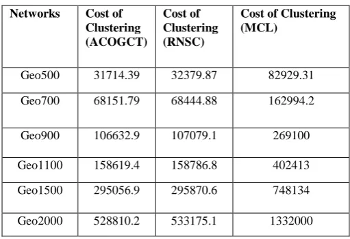
Table 1. Cost of Clustering with increasing Graph Size of RGG

Networks Cost of Clustering (ACOGCT)

Cost of Clustering (RNSC)

Cost of Clustering (MCL)

Geo500 31714.39 32379.87 82929.31 Geo700 68151.79 68444.88 162994.2

Geo900 106632.9 107079.1 269100

Geo1100 158619.4 158786.8 402413 Geo1500 295056.9 295870.6 748134

Geo2000 528810.2 533175.1 1332000

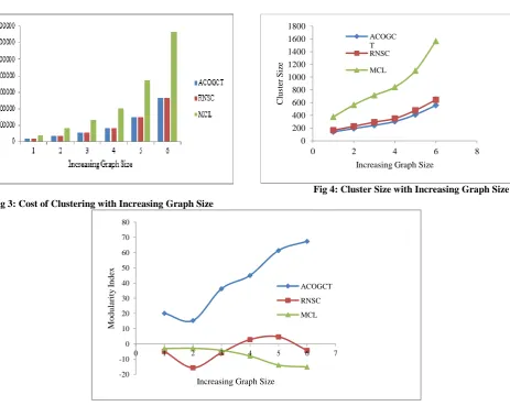
It is observed from figure 3 that the cost of clustering, produced by these graph clustering algorithms is always increased with increasing of graph size for all the test cases used here for conducting the experiments. ACOGCT is showing better results in cost evaluation compared to RNSC and MCL. MCL is giving the costliest clustering results compared to ACOGCT and RNSC. But RNSC is less costly compared to MCL.

It can be established from the observations that ACOGCT is generating lower-cost clustering results compared to RNSC and MCL.

( )

{ q| {1,.., }} q r

 

( )a h

n

c

_h

( )a



( )b l

n

l

c



( )b

,

h l

n h

c



( )a

l

c

( )b

4.2.2 Cluster Size

The cluster size values, resulted after clustering on synthetic RGG, are kept in table 2. All the computations are performed on synthetic RGG with increasing graph size.

Table 2. Cluster size with increasing Graph Size of RGG

Network Cluster Size (ACOGCT)

Cluster Size (RNSC)

Cluster Size (MCL)

Geo500 141 166 375

Geo700 193 228 563

Geo900 243 293 714

Geo1100 303 350 843

Geo1500 410 478 1100

Geo2000 557 644 1565

Fig 4 shows that cluster size prediction is nearly reaching the highest accuracy in case of ACOGCT compared to RNSC and MCL. This implies that the rate of increment in cluster size with increasing of graph size is proper for ACOGCT. MCL is generating huge number of clusters compared to ACOGCT and RNSC. MCL is not giving meaningful clusters. MCL is not behaving well in producing clusters. RNSC’s cluster size prediction is better compared to MCL.

It can be concluded that ACOGCT is producing meaningful and significant clusters compared to RNSC and MCL.

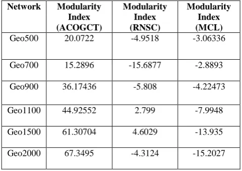
4.2.3 Modularity Index

[image:8.595.60.524.82.451.2]

Table3 represents the modularity index values which are computed using the clustering results, produced by ACOGCT, RNSC and MCL algorithm. The evaluation of modularity is done using synthetic RGG with increasing graph size. Modularity Index is an important performance metric to test accuracy of clustering results of different graph clustering algorithms. The accuracy is measured based on the strength of the clusters, produced during clustering. The strength is computed based on the dense intra-cluster connectivity and sparse inter-cluster connectivity.

Fig 3: Cost of Clustering with Increasing Graph Size

Fig 4: Cluster Size with Increasing Graph Size

0 200 400 600 800 1000 1200 1400 1600 1800

0 2 4 6 8

C

lu

st

er

S

iz

e

Increasing Graph Size

ACOGC T RNSC MCL

Fig 5: Modularity with Increasing Graph Size

-20 -10 0 10 20 30 40 50 60 70 80

0 1 2 3 4 5 6 7

M

o

d

u

la

ri

ty

I

n

d

ex

Increasing Graph Size

[image:9.595.47.287.113.282.2]

Table 3. Modularity of Clustering with increasing Graph Size of RGG

Network Modularity Index (ACOGCT) Modularity Index (RNSC) Modularity Index (MCL)

Geo500 20.0722 -4.9518 -3.06336

Geo700 15.2896 -15.6877 -2.8893

Geo900 36.17436 -5.808 -4.22473

Geo1100 44.92552 2.799 -7.9948

Geo1500 61.30704 4.6029 -13.935

Geo2000 67.3495 -4.3124 -15.2027

Figure 5 shows that ACOGCT is behaving more modular or producing more strong clusters compared to RNSC and MCL. ACOGCT’s modularity curve is gradually increasing with increasing of graph size. The modularity is decreasing gradually with increasing of graph size in case of MCL. RNSC is achieving better modularity compared to MCL. ACOGCT gains positive impact on modularity index evaluation for all the test cases. It can be stated that ACOGCT is producing more accurate clusters compared to RNSC and MCL.

4.3

Evaluation on Real RGG Graphs

For this evaluation ‘bork2455’, 2002, high confidence yeast protein interactions by von Mering et al. and “shen-orr”, 2002, network motifs in the transcriptional regulation network of Escherichia coli by Shen-Orr et al. are taken and the performance of these algorithms is tested on these graphs. The clustering results are tabled in the following table 4. The computed results show that the cost of clustering produced by ACOGCT is lower compared to RNSC and MCL. The computed modularity of clustering results of the algorithms is produced and ACOGCT and RNSC are gaining positive index whereas MCL is at negative index. However, ACOGCT is achieving high modularity index compared to RNSC’s index. The cluster size prediction of ACOGCT is more significant and accurate compared to RNSC and MCL. RNSC is producing more number of clusters compared to ACOGCT and MCL. The computed cluster size of MCL tells that MCL is not exploring the whole network. It is observed from the results, shown in table 4 that ACOGCT is more accurate and significant in producing lower-cost clusters compared to RNSC and MCL.

4.4 NMI Value on Real RGG

NMI is playing a vital role to determine the quality of clusters, produced by clustering algorithms. The quality is measured in terms of optimality and it is basically achieved through the information passing between clustering results of a clustering algorithm. It is act as an information theoretic measure and shows the value of mutual information sharing between two clusterings of an algorithm.

It is observed from figure 6 that NMI value is highest in case of ACOGCT compared to RNSC and MCL. ACOGCT produces high quality clusters compared to RNSC and MCL whereas the clusters evaluated from MCL clustering results are not meaningful. However, RNSC is producing optimal clusters compared to MCL. The figure 6 is plotted using NMI value and mixing parameter (mu) of network. The mixing parameter (mu) value is set in the range of 0.1 to 0.9. After 300, 500, 700 runs with using real RGG graph (bork2455 [55]), NMI value is computed in case of ACOGCT and RNSC and for the case of MCL; experiments are conducted by changing the inflation value as I= {2.5, 3.5, 4.5}.

Fig 6: NMI value on Real RGG Data (bork2455)

0.84 0.86 0.88 0.9 0.92 0.94 0.96 0.98 1

0 0.2 0.4 0.6 0.8 1

N M I V al u e mu ACOGCT RNSC MCL

Table 4. Clustering results of these algorithms on real RGG

Ne two rk Co st o f Clu ste rin g (AC O G CT) Co st o f Clu ste rin g (RN S C) Co st o f Clu ste rin g (M CL) Mo d u la rity (AC O G CT) Mo d u la rity (RN S C) Mo d u la rity (M CL) Clu ste r-S ize (AC O G CT) Clu ste r S ize (RN S C) Clu ste r S ize (M CL) bork245 5 [55] 116758.092 7 121607. 5318 324408. 6402

71.6785 13. 4137

-32. 4219

336 393 337

Shen-orr [56]

37063.758 38306.0167 59486.9863 21.685 -171.3135

9

-21.070

67

[image:9.595.35.288.139.525.2]

The NMI value curve shows that the optimality in steadily increased with increasing of mu and when mu>=0.6 the NMI is increasing gradually and it is very close to 1 in case of ACOGCT. RNSC and MCL are not showing that type of behaviour. RNSC’s NMI curve is growing linearly with increasing of mu. However, NMI value computation of RNSC shows that RNSC is better in producing optimal clusters than MCL. MCL is behaving opposite of ACOGCT in NMI computation. MCL’s NMI curve is decreasing in between 0.1 and 0.5 of the mu value and afterwards it is linearly going. It can be established from the observations that the mutual information sharing between clusterings is more effective and significant in case of ACOGCT whereas MCL can’t provide good quality clusters due to the less NMI value. MCL is not giving accuracy in producing optimal clusters compared to RNSC also. It can be concluded that ACOGCT is producing meaningful and expressive clusters compared to RNSC and MCL. ACOGCT is more optimal compared to RNSC and MCL.

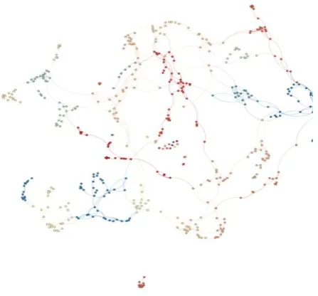
[image:10.595.361.535.115.248.2]

4.5 Visualization of Clustering of Real RGG

Bork and Synthetic Graphs

Fig 7 and fig 11 signify the visual representation of real RGG (bork2455) and (shen-orr) respectively with huge interactions exist between the nodes. Fig 15, fig16 and fig 17 shows the visual presentation of synthetic network with 1500, 900 and 700 nodes respectively. The visualization of clustering results, produced by ACOGCT, RNSC and MCL on real RGG (bork2455) are shown in the figure 10, figure 9 and figure 8 respectively. The resulted clustering visualizations, produced by ACOGCT, RNSC and MCL on shen-orr real RGG are shown in the following figure 12, figure 13 and figure 14. It can be resolved from the visualizations of clustering results for both the real RGGs that ACOGCT’s clusters are more expressive and meaningful compared to RNSC and MCL. RNSC is performing better in producing clusters compared to MCL for all the test cases. It can be clearly assumed from the entire MCL’s clustering that clusters are not properly visible and incorrect. RNSC is producing more optimal clusters compared to MCL. But the clusters, resulted from ACOGCT’s clustering, are more accurate and proper compared to RNSC and MCL. ACOGCT is generating more optimal clusters compared to RNSC. ACOGCT is achieving significant improvement in producing optimal clusters for real large networks. All the visualizations of networks and clusterings are modularity controlled as they are shown in the following figure 18-23. Modularity is capable of identifying nodes which are in the same cluster using the help of some similarity measures i.e. basically determined using various properties of a complex network. It is perceived from fig 18 and fig 21 that clusters are marked appropriately by modularity approach in case of ACOGCT. RNSC and MCL are not responding well in that situation compared to ACOGCT. RNSC is behaving better compared to MCL in identification of clusters. The modularity approach is identifying the clusters, produced by ACOGCT accurately and the clusters are more expressive and significant compared to RNSC and MCL.

Fig 7: Visualization of RGG bork2455 [55]

[image:10.595.340.506.324.485.2]

Fig 8: Visualization of RNSC’s clustering Results on bork2455 [55]

[image:10.595.358.526.529.696.2]

[image:11.595.55.524.75.768.2] [image:11.595.363.518.105.220.2]

Fig 11: Visualization of RGG shen-orr [56]

[image:11.595.338.490.314.478.2]

Fig 12: Visualization of ACOGCT’s clustering Results on shen-orr [56]

[image:11.595.74.205.357.496.2]

Fig 13: Visualization of RNSC’s clustering Results on shen-orr [56]

Fig 14: Visualization of MCL’s clustering Results on shen-orr

Fig 15: Visualization of synthetic RGG with 1500 nodes

[image:11.595.338.524.555.750.2] [image:11.595.84.224.609.741.2]

[image:12.595.38.228.66.261.2] [image:12.595.304.511.82.281.2]

Fig 17: Visualization of synthetic RGG with 700 nodes

Fig 19: Modularity based clusters identifying in RNSC’s clustering on bork2455 [55]

Fig 20: Modularity based clusters identifying in MCL’s clustering on bork2455 [55]

[image:12.595.38.255.332.472.2]

Fig 21: Modularity based clusters identifying in ACOGCT’s clustering on shen-orr [56]

[image:12.595.323.544.336.485.2]

Fig 16: Visualization of synthetic RGG with 900 nodes

[image:12.595.297.529.554.708.2] [image:12.595.35.255.558.708.2]

5. CONCLUSIONS

There is an emerging issue in clustering of complex networks in the field of science and engineering. In this work, we have proposed an advanced and accurate cost based graph clustering technique, to investigate high quality clusters in large-scale RGG networks starting from a greedy creation of initial clustering scenario. The developed algorithm is basically a modified form of RNSC and some additional features as the aspiration criteria based tabu evaluation, etc. have been adopted to achieve more efficiency in graph clustering in terms of robustness and optimality. This developed algorithm has key benefits over existing graph clustering algorithms on the basis of lower cost cluster generation. We have shown that our developed algorithm can reliably and sensitively extract lower-cost clusters from artificially generated RGG networks. The modified algorithm gains immense relevance in the real world situation as presented in this work. Visualizations of the resulted clusterings, produced by our developed algorithm and some baseline methods affirm that the developed algorithm is generating more expressive and significant clusters compared to other baseline methods. Scale cost evaluation is O (n) in RNSC. This can easily be done in O (1) time if the information about current node, and its cluster contribution are pre-computed and these features are incorporated in our developed algorithm. The developed algorithm can be further extended by a parallel move technique which will give better results in the case of run-time. This algorithm can be further applied to various applications as wireless ad-hoc and sensor networks.

6.

ACKNOWLEDGMENTS

The first author would like to thankfully acknowledge the research scholarship awarded by Banaras Hindu University, Varanasi.

7.

REFERENCES

[1] Barabási , A.L., Albert, R., 2002. Statistical mechanics of complex networks. Rev. Mod. Phys.74, 0034-6861, 47.

[2] Dorogovtsev, S.N., Mendes, J.F.F. 2003. Evolution of Networks: From Biological Nets to the Internet and WWW, Oxford University Press.

[3] Boccaletti , S., et al., Complex networks: Structure and dynamics - FTP Directory Listing. 2006. Phys. Rep. 424 , 175, 175–308.

[4] Newman, M.E.J. 2003. The structure and function of complex networks. SIAM Rev. 45, 167, 167-256. [5] Watts, D.J. 2004. The “New” Science of Networks.

Annu. Rev. Soc. 30, 243, 243-270.

[6] Rapoport, A., Horvath, W.J. 1961. A study of a large sociogram, Behavioral Science 6,279–291.

[7] Yu, Z., Wong, H.S., Wang, H. 2007. Graph-based consensus clustering for class discovery from gene expression data, Bioinformatics 23, 2888–2896. [8] Bandyopadhyay, S., Mukhopadhyay, A., Maulik, U.

2007. An improved algorithm for clustering gene expression data, Bioinformatics 23, 2859–2865.

[9] Barabasi, A.-L., Albert, R., Jeong, H. 2000. Scale-free characteristics of random networks: the topology of the World-Wide Web, Physica A: Statistical Mechanics and its Applications 281 (1–4), 69–77.

[10] Kleinberg, J.M., Kumar, R., Raghavan, P., Rajagopalan, S., Tomkins, A.S. 1999. The Web as a graph: measurements, models, and methods. Computing and Combinatorics: 5th Annual International Conference, COCOON’99, Proceedings, Tokyo, Japan, pp. 1–17. [11] Kumar, R., Raghavan, P., Rajagopalan, S., Sivakumar,

[image:13.595.299.554.87.259.2]

D., Tomkins, A., Upfal, E. 2000. Stochastic models for the Web graph. FOCS’00: Proceedings of the 41st Annual Symposium on Foundations of Computer Science, IEEE Computer Society, Washington, DC, USA, p. 57.

Fig 22: Modularity based clusters identifying in RNSC’s

[image:13.595.39.260.96.244.2]

[12] Adamic, L.A., Huberman, B.A. 2000. Power-law distribution of the World Wide Web. Science 287, 2115. [13] Newman, M.E.J., Strogatz, S.H., Watts, D.J. 2001.

Random graphs with arbitrary degree distributions and their applications, Physical Review E 64 (026118). [14] Watts, D.J., Strogatz, S.H. 1998. Collective dynamics of

‘small-world’ networks. Nature 393 (6684) 440–442. [15] White, J.G., Southgate, E., Thomson, J.N., Brenner, S.

1986. The structure of the nervous system of the nematode Caenorhabditis elegans. Philosophical Transactions of the Royal Society of London Series B-Biological Sciences 314 (1165) 1–340.

[16] Camacho, J., Guimera, R., Amaral, L. 2002. Robust patterns in food Web structure. Physical Review Letters 88 (22).

[17] Guelzim, N., Bottani, S., Bourgine, P., Kepes, F. 2002. Topological and causal structure of the yeast transcriptional regulatory network, Nature Genetics 31, 60–63.

[18] Barabási, A.L., Albert, R. 1999. Emergence of Scaling in Random Networks. Science 286, 509-512.

[19] Milo, R., Shen-Orr, S., Itzkovitz, S., Kashtan, N., Chklovskii, D., Alon, U. 2002. Network Motifs: Simple Building Blocks of Complex Networks. Science 298, 824-827.

[20] Alon, U. 2007. The impact of cellular networks on disease comorbidity. Nat. Rev. Gen. 8, 450-461.

[21] Ravasz, E., Somera, A.L., Mongru, D.A., Oltvai, Z.N., Barabasi, A.-L. 2002. Hierarchical Organization of Modularity in Metabolic Networks. Science 297, 1551-1555.

[22] Brandes, U., Math , J. 2001. A Faster Algorithm for Betweenness Centrality. Sociol. 25, 163-177.

[23] Holme, P., Kim, BJ, Yoon, CN, Han, SK. 2002. Attack vulnerability of complex networks, Phys. Rev. E 65, 056109.

[24] Duncan, S. Callaway, John, Hopcroft, E., Kleinberg, Jon M., Newman, M. E. J., and Strogatz, Steven H. 2001. Are randomly grown graphs really random? Physical Review E, 64:041902.

[25] B´ela Bollob´as. 1985. Random Graphs. Academic Press.

[26] Kirkpatrick, Scott and Selman, Bart. 1994. Critical behavior in the satisfiability of random boolean expressions. Science, 264:1297– 1301.

[27] Gilbert, E. N. 1961. Random Plane Networks. Journal of the Society for Industrial and Applied Mathematics, 9(4):533–543.

[28] Watts, Duncan J. and Strogatz, Steven H. 1998. Collective dynamics of ‘small-world’ networks. Nature, 393(4):440–442.

[29] Newman, M., Watts, D, and Strogatz, S. 2002. Random graph models of social networks. In Proc. Natl. Acad. Sci, volume 99, pp. 2566–2572.

[30] Barabasi Albert-Laszlo, Crandall, R. E. 2003. Linked: The New Science of Networks. American Journal of Physics, 71(4):409–410.

[31] Penrose, Mathew D. 2003. Random Geometric Graphs. volume 5 of Oxford Studies in Probability. Oxford University Press.

[32] Cohen, Reuven, Erez, Keren, Avraham, Daniel, ben and Havlin, Shlomo. 2000. Resilience of the Internet to Random Breakdowns. Physical Review Letters, 85:4626–4628.

[33] Albert, R´eka. 2000. Hawoong Jeong, and Albert- L´aszl´o Barab´asi. Error and attack tolerance of complex networks. Nature, 406:378–382.

[34] Krapivsky, P. L., Redner, S., and Leyvraz, F. 2000. Connectivity of Growing Random Networks. Physical Review Letters, 85:4629– 4632.

[35] Albert, R´eka and Barab´asi, Albert-L´aszl´o. 2000. Topology of Evolving Networks: Local Events and Universality. Physical Review Letters, 85:5234–5237. [36] Dorogovtsev, S. N. and Mendes, J. F. F. 2000. Evolution

of networks with aging of sites. Physical Review E, 62:1842–1845.

[37] Watts, Duncan J. and Strogatz, Steven H. 1998. Collective dynamics of ‘small-world’ networks. Nature, 393:440–442.

[38] Watts, D. J. 1999. Small Worlds. Princeton University Press.

[39] Newman, M. E. J. and Watts, D. J. 1999. Scaling and percolation in the small-world network model. Physical Review E, 60:7332–7342.

[40] Newman, M. E. J. 2000. Models of the small world. Journal of Statistical Physics, 101:819–841.

[41] Banavar, Jayanth R., Maritan, Amos, and Rinaldo, Andrea. 1999. Size and form in efficient transportation networks. Nature, 399:130– 132.

[42] Xia, W. and Thorpe, M. F. 1988. Percolation properties of random ellipses. Physical Review A, 38(5):2650– 2656.

[43] Balberg, I. 1985. Universal percolationthreshold limits in the continuum. Physical Review B, 31:4053–4055. [44] Jund, Philippe, Jullien, R´emi, and Campbell, Ian. 2001.

Random walks on fractals and stretched exponential relaxation. Physical Review E, 63:036131.

[45] Pastor-Satorras, Romualdo and Vespignani, Alessandro. 2001. Epidemic Spreading in Scale- Free Networks. Physical Review Letters, 86:3200–3203.

[46] Donath, W.E. and Hoffman, A.J. 1973. Lower Bounds for the Partitioning of Graphs. IBM J. Research and Development, vol. 17, pp. 422- 425.

[47] Hall, K.M. 1970. An R-Dimensional Quadratic Placement Algorithm. Management Science, vol. 11, no. 3, pp. 219-229.

[48] Ng, A.Y., Jordan, M., and Weiss, Y. 2001. On Spectral Clustering: Analysis and an Algorithm. Proc. 14th Advances in Neural Information Processing Systems (NIPS ’01).

[49] King, Andrew Douglas. 2004. Graph Clustering with Restricted Neighbourhood Search, M.S Thesis, University of Toronto.

[50] Dongen, S. M. van. 2002. Graph Clustering by Flow Simulation. PhD thesis, University of Utrecht.

[52] Mladenovi´c, N. and Hansen , P. 1997. Variable neighbourhood search, Computers and Operations Research, 24(11):1097–1100.

[53] NEWMAN, M. E. J. AND GIRVAN, M. 2004. Finding and evaluating community structure in networks.Physical Review E 69, 026113.

[54] Kvalseth, T. O., 1987. Entropy and correlation: Some comments. Systems, Man and Cybernetics, IEEE Transactions, 17(3):517–519.

[55] Von Mering,C., Krause, R., Snel, B., Cornell, M., Oliver, S.G., Fields, S. and Bork, P. 2002. Comparative

assessment of large-scale data sets of protein-protein interactions. Nature, 417, 399-403.

[56] Shai S. Shen-Orr, Ron Milo, Shmoolik Mangan & Uri Alon. (2002) Network motifs in the transcriptional regulation network of Escherichia coli. Nature 31,64-68. [57] Dhara, Mousumi and Shukla, K. K.. 2012. Performance