Fundamental equilibrium exchange rate for the Polish zloty

Munich Personal RePEc Archive

Fundamental equilibrium exchange rate

for the Polish zloty

Rubaszek, Michal

September 2005

Online at

https://mpra.ub.uni-muenchen.de/126/

Fundamental equilibrium exchange

rate for the Polish zloty

Micha∏ Rubaszek – Economist, Macroeconomic and Structural Analysis Department, National Bank of Poland and Econometrics Institute, Warsaw School of Economics.

E-mail: Michal.Rubaszek@mail.nbp.pl

The opinions expressed in this paper are those of the author and should not be treated as the official position of the National Bank of Poland.

Author would like to thank Ryszard Kokoszczyƒski, Rebecca Driver, Jakub Borowski, Marek A. Dàbrowski and NBP economists for many useful comments that helped to improve the previous versions of this paper.

Design:

Oliwka s.c.

Layout and print:

NBP Printshop

Published by:

National Bank of Poland

Department of Information and Public Relations 00-919 Warszawa, 11/21 Âwi´tokrzyska Street phone: (22) 653 23 35, fax (22) 653 13 21

© Copyright by the National Bank of Poland, 2005

Contents

Tables and figures

4

Abstract

5

Introduction

6

1. The model of fundamental equilibrium exchange rate

7

2. Three inputs of the fundamental equilibrium exchange rate model

12

2.1. Foreign trade model . . . 12

2.1.1. Export and import volumes of goods and services . . . 12

2.1.2. Export and import prices of goods and services . . . 14

2.1.3. Simulations . . . 15

2.2. Internal equilibrium . . . 15

2.3. External equilibrium . . . 16

3. The results

19

3.1. The level of the zloty’s fundamental equilibrium exchange rate . . . 19

3.2. Sensitivity analysis . . . 20

3.2.1. Foreign output gap . . . 21

3.2.2. Domestic output gap . . . 21

3.2.3. Target level of balance on trade and services . . . 22

4. Summary

24

Tables and figures

Tables and figures

Table 1Countries’ share in the Polish foreign trade (%) . . . 13

Table 2Cointegration trace test . . . 14

Table 3An impact of 10% permanent depreciation of the RER on foreign trade . . . 15

Table 4Methods to estimate the output gap . . . 16

Table 5Balance on goods and services and output gap in Poland in 2004 . . . 20

Figure 1Domestic demand and real exchange rate . . . 11

Figure 2Output gap in Poland and in its main trading partners . . . 16

Figure 3Sensitivity of the zloty’s misalignment with respect to the assumed level of the foreign output gap . . . 21

Figure 4Sensitivity of the zloty’s misalignment with respect to the assumed level of the domestic output gap . . . 22

Figure 5The domestic demand and the real exchange rate in response to an increase in assumed level of domestic output gap . . . 22

Figure 6Sensitivity of the zloty’s misalignment with respect to the assumed value of the balance on transfers . . . 23

Abstract

In May 2004 Poland joined the European Union and is thereby committed to introduce the euro in the forthcoming years. The balance of costs and benefits of the euro adoption depends on the decision of the Polish and European authorities concerning the level of central parity in the ERM II, and subsequently the conversion rate of the zloty. In order to address the issue of an "ideal" level of the real exchange rate this paper proposes a model which is applied to estimate the level of the equilibrium of the zloty. The results indicate that at the end of 2004 the zloty was undervalued by 4.3%.

JEL classification: F12, F31, F41

1

Introduction

Introduction

The studies of the development tendencies in the Polish economy in the late 1990s and at the beginning of this millennium cannot neglect the influence of the foreign sector on the economic situation of the country. In this period Polish current and capital accounts were fully liberalised. The Polish economy became more open: the volume of imports and exports multiplied five and threefold, respectively (Mroczek, Rubaszek, 2003 and 2004). As a consequence, the impact of exchange rate fluctuations on Polish economy increased considerably.

In May 2004 Poland joined the European Union and thus became obliged to introduce the euro in the forthcoming years. Among the benefits of joining the Monetary Union, which are discussed in Borowski (2004), one can number lower costs of borrowing, elimination of the exchange rate risk, better access to foreign capital and lower transaction costs. These advantages of the single currency seem to outweigh its major cost, i.e. loss of monetary policy independence. The balance of costs and benefits of euro adoption also depends on the decision of the Polish and European authorities concerning the level of the central parity in the ERM II, and subsequently the conversion rate of the zloty. More precisely, inappropriate determination of the conversion rate may invoke severe consequences for the real sector of Polish economy. On the one hand, an overvalued rate leads to a loss of competitiveness of domestic producers and hence forces them to limit their output or even may drive them bankrupt. If prices are sticky and the adjustment slow, an overvalued conversion rate may dampen domestic output for a prolonged period of time. On the other hand, an undervalued rate results in ineffective allocation of capital as the companies that are not competitive can expand their activity. Moreover, the purchasing parity of domestic wages is subdued, which might not optimise consumers’ welfare. Finally, weak currency brings about inflationary pressure, which in an environment of externally set nominal interest rates may lead to an unsustainable consumption boom. The above considerations lead us to the conclusion that the conversion rate should equal the equilibrium exchange rate of the zloty to maximise the net gain of adopting the euro.

In the case of the central parity in the ERM II the problem is more complicated. It may occur that setting the entry rate at the equilibrium level may be suboptimal. An overvalued parity could be a better choice in the situation of excessive inflation, for instance. An undervalued parity would be recommended if domestic demand was subdued. It should be emphasised, however, that misaligned ERM II parity may entail speculative attacks that would lead to severe problems with maintaining the zloty within the fluctuation bands.

In order to address the issue of an “ideal” level of the real exchange rate this paper describes one of the most popular methods of the equilibrium exchange rate calculation, namely the model of fundamental equilibrium exchange rate (FEER, Williamson 1983). A modification of this model is used to estimate the equilibrium level of the zloty in the forth quarter of 2004. It was found that in this period the quarterly average value of the real effective rate of the zloty was 4.3% weaker than its fundamental value. This result, however, is subject to uncertainty as it depends on a set of assumptions. In order to address this issue a thorough sensitivity analysis was performed. Among others, the impact of EU transfers on the level of the equilibrium exchange rate was investigated.

2

1

The model of fundamental equilibrium exchange rate

The fundamental equilibrium exchange rate model is probably the most popular method of calculating the equilibrium exchange rate (MacDonald 2000). On the basis of this model, which is also referred to as the internal-external balance model, it is possible to compute the level of the real exchange rate that is consistent with simultaneous attainment of the internal and external equilibria. In this paper, the internal equilibrium means that the actual output is equal to its potential level, i.e. the output gap is null. The external equilibrium is defined as attainment of some target level of the current account balance that corresponds to optimal portfolio allocation. In this sense, the fundamental equilibrium exchange rate may be characterised as the level of the exchange rate that is consistent with ideal macroeconomic performance (Williamson 1994, p. 180). It should be pointed out that in the short-term horizon the FEER might not be the optimal level of the exchange rate if the economy is not in the equilibrium. Take a temporary undervalued exchange rate for instance: it would be recommended in case of a weak domestic output. By contrast, a temporary overvaluation would be helpful to contain inflationary pressure.

According to MacDonald (2000) there are two methods of estimating the fundamental equilibrium exchange rate. The first one is based on a full-scale macroeconomic model. The FEER is the level of the exchange rate that would remain if all markets were in equilibrium. The advantage of this approach is that most of the model’s variables are endogenous and thus the calculated exchange rate is consistent with a well defined economic equilibrium. Moreover, on the basis of such model one can calculate the short-term dynamics towards the long-term steady-state. The disadvantage of this approach is that it requires a sophisticated macroeconomic model, which has a well-defined steady-state solution. In practice, the construction of such a model tends to be very difficult and time-consuming. Moreover, the final results might be non-transparent, especially if the model is very complex. The alternative and less sophisticated partial equilibrium approach limits the group of endogenous variables to a few variables related to foreign sector of the economy. It means that domestic prices, domestic demand, employment, money supply and other quantities are treated as exogenous. In this approach, one focuses solely on the external equilibrium condition, with the exchange rate functioning as a control variable. More precisely, partial-approach FEER is the level of exchange rate that makes the current account balance equal to its target level, given that other markets are in equilibrium. The main shortcoming of the partial equilibrium model is that it does not explain the behaviour of the whole economy and does not provide any information about the short-term dynamics. Its major advantages over the full-equilibrium approach are simplicity and transparency.

1

The model of fundamental equilibrium exchange rate

It should be emphasised, that in equilibrium, the level of domestic demand may depend on the level of real exchange rate. Let us take the terms-of-trade effect for instance: real exchange rate appreciation leads to an improvement of the terms-of-trade and consequently in order to finance a given amount of imports a country can export less. This allows for domestic demand expansion. This effect for Germany was found by Meier (2004). As our model can be classified as partial equilibrium, in order to keep its small size and transparency we assume that domestic demand and real exchange rate are independent. A detailed description of the model is presented below.

Goods markets at home and abroad are in equilibrium, when the actual output (Y) is equal to its potential level ( ). Therefore, the internal equilibrium condition is met when:

(1)

, (2)

where “*” stands for foreign variables.

The real sector in our model is described by two identities and two behavioural equations. In equations (3) and (4) the domestic output (Y) is defined as the sum of domestic demand (DD) and net exports (NT), where net exports is the difference between exports (X) and imports (M):

(3)

. (4)

It is supposed that in the long run the level of domestic exports (XS) is determined by supply factors, as Poland is a small open economy. If companies produce subject to the transformation function with constant transformation elasticity (α1) then the first-order condition of profits maximisation leads to the following relationship between exports, domestic output and relative prices1_:

, α0>0 α1>0 (5)

where PX and Pstand for export and domestic prices, respectively. In the short run, the

deviation of the actual exports from its supply level given by (5) depends on demand factors, such as the foreign demand and price competitiveness of domestic exports on the foreign market:

, f1>0, f2<0 (6) where P*/Sis the level of foreign prices expressed in units of domestic currency.

Subsequently, the level of domestic imports is entirely determined by demand factors as it is supposed that the foreign supply is infinite. As imported and domestically produced goods are assumed to be imperfect substitutes and the utility function is in CES form, the first-order condition of the utility maximisation leads to the following relationship between imports, total demand and relative prices:

, β0>0, β1>0 (7) where PMstands for import prices.

The external equilibrium in the model is defined as attainment of some target level of the current account balance:

, (8)

where CABand TCABare actual and target levels of the current account balance, respectively. One can notice that as the internal and external equilibria are expressed in flow terms, the fundamental equilibrium exchange rate is a medium-term concept.

CAB=TCAB M P tariff

P Y

M

=β0_ + _−β

1 1

( )

X X f

Y Y

P tariff P S

S

X

= ( , ( + )

/ )

*

* *

1

X P P Y

S₌  X

 

α0 α

1

NT= −X M Y=DD+NT Y*₌Y*

Y=Y

Y

2

The nominal sector in the model is described by three identities and two behavioural equations. The current account balance is the sum of three components: the trade balance (CAB_TB)2, the balance on income (CAB_INC) and the balance on transfers (CAB_TRANS).

. (9)

The trade balance is the difference between the nominal exports and the nominal imports:

. (10)

The third identity relates the nominal output to the product of the real output and domestic prices:

. (11)

The two behavioural equations are related to export and import prices. Assuming that the “price taker – price maker” hypothesis holds, these indices can be expressed as a weighted average of domestic and foreign prices:

, γ0>0, γ1∈<0,1> (12) . δ0>0, δ1∈<0,1> (13) For countries that are price makers the elasticities γ1and δ1are close to unity. By contrast, the price taker economies are characterised by values of these parameters close to zero.

Finally, let us define the real exchange rate (Q) as a relative price of domestic goods to foreign goods:

, (14)

where an increase in Sand Qstands for appreciation in the domestic currency.

On the basis of the above system, which is described by equations (1)–(14), one can estimate the levels of the domestic demand (DD) and the real exchange rate (Q) that would ensure the occurrence of the internal and external equilibria. These “ideal” values of the domestic demand and the real exchange rate, which will be referred to as DDFEERand QFEER, depend on the assumed values of the exogenous variables, namely the target level of the current account, the balance on transfers, potential outputs and others.

The solution of the above system is as follows. On the basis of the equations (12), (13) and (14) one can calculate that the relative prices that have an impact on the export and import volumes according to (5), (6) and (7) depend solely on the level of the real exchange rate:

(15)

(16)

(17)

Equation (15) states that the appreciation of the real exchange rate leads to a fall in the profitability of exports. In effect, the level of exports is declining in line with the relationship (5). The price competitiveness of home-produced goods on foreign markets is also deteriorating in response to the strengthening of the domestic currency, which is shown in (16). Consequently, the demand for exports is falling in line with the relationship (6). Finally, according to the equation (17), the price competitiveness of the imported goods is rising in response to a real exchange rate appreciation. As a result, the volume of imports is increasing (see eq. 7).

P P

P P S

P Q

M

=δ0 δ −δ =_δ δ−

1 0 1 1 1 1 ( */ )( ) ( ) P P S

P P S

P S Q

X * * ( ) * / ( / ) /

=γ0 γ −γ =γ γ

1 0 1 1 1 P P

P P S

P Q

X

=γ0 γ −γ =_γ γ−

1 0 1 1 1 1 ( */ )( ) ( ) Q P P S = * /

PM_=δPδ P S −δ 0

1

1₍ *_{/ )}( 1)

PX_=γ Pγ P S −γ 0

1

1₍ *_{/ )}( 1)

Y_N=PY

CAB TB_ =P XX −P MM

CAB=CAB TB_ +CAB INC_ +CAB TRANS_

1

The model of fundamental equilibrium exchange rate

It can be concluded that the appreciation entails a decrease in exports and an increase in import volumes and thus it deteriorates net exports. Furthermore, if in the identity (4) Xand Mare substituted by the expressions (5) and (7), and the relationships (1), (14) and (16) are taken into account, one can calculate that in the long-run net exports (NTLR) equal to3:

. (18)

This expression can be transformed so that in the long run the ratio of net exports to output depends solely on the level of the real exchange rate:

, (19)

where the first derivative:

. (20)

In the short-term horizon, apart from the real exchange rate, net exports are also determined by other factors, namely domestic and foreign demand (see equations 3–7):

. g₁<0, g2∈(-1, 0), g₃>0 (21)

The partial derivative with respect to domestic demand is greater than -1 to ensure that the growth of domestic demand has a positive impact on the total output, i.e. .

Let us now focus on the trade balance, which is described by the identity (10). If the values of X, M, PXand PM are taken from the expressions (5), (7), (14) and (16), respectively, and the

condition (1) holds, one can express the long-term value of this balance as:

. (22)

This expression can be transformed so that in the long run the ratio of the trade balance to the nominal output depends solely on the level of the real exchange rate:

. (23)

The sign of the first derivative:

(24)

may be ambiguous. We assume that the values of the relevant parameters ensure that this expression is negative and hence the Marshall-Lerner condition holds.

In the short-term horizon, apart from the real exchange rate, the trade balance is also determined by other factors like the demand at home and abroad:

, h1<0, h2<0, h3>0. (25) In accordance with the equations (1), (3) and (21) the levels of the real exchange rate (Q) and domestic demand (DD) that would ensure the occurrence of the internal equilibrium can be calculated. In equilibrium, in order to guarantee that the actual output equals its potential level, a rise in domestic demand requires a fall in net exports of the same value. This implies that domestic currency must appreciate. As a result, the real exchange rate is an increasing function of the domestic demand:

, where _∂∂Q > (26)

DD 0 Q=ie DD( ,...

CAB TB_ ₌h Q DD Y( , , *,...)

d CAB TB Y

dQ Q Q

LR N

( _ / )

( )( ) ( ) ( )( ) ( )( ) ( ) ( )( )

=_α +_{α γ} − _γ +α +α γ− − −_β −_{β δ} − _δ −β −β δ− −

0 1 1 0

1 1 1 1

0 1 1 0

1 1 1 1

1 1 1 1 1 1 1 1 1 1

CAB TBLR Y Q Q

N

_ / =α γ0

(

)

(

)

0 0

11

1 1 1 1

CAB TBLR Q PY Q PY

_ =α γ0

(

)

(

)

0 0

11

1 1 1 1

dY dDD>0 NT=g Q DD Y( , , *,...)

d NT Y

dQ Q Q

LR

( / )

( ) ( ) ( ) ( )

=_{α α γ} − _γα α γ− − +_{β β δ} − _δ−β −β δ− − <

0 1 1 0

1 1

0 1 1 0

1 1

1 1 1 1 1 1 1 1 0

NTLR Y Q Q

/ =α γ0

(

)

(

)

0 0

1

1 1 1 1

NTLR_{=α γ}

(

)

(

)

0 0

1

0 0

1

1 1 1 1

2

Reasoning in the similar way, on the basis of the equations (8), (9) and (23) one can calculate the levels of the real exchange rate (Q) and the domestic demand (DD) that would ensure the occurrence of the external equilibrium. Higher domestic demand worsens the trade balance and hence the real exchange rate must depreciate so that the current account balance returned to its target level. Consequently, the real exchange rate is a decreasing function of the domestic demand:

, where (27)

The intercept of the two curves given by (26) and (27) determines the fundamental levels of the real exchange rate (QFEER) and the domestic demand (DDFEER):

(28)

(29)

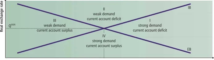
Corresponding to the presented model, one can see that various combinations of the domestic demand and the real exchange rate may result in different types of disequilibria. These disequilibria as well as the fundamental equilibrium values of the exchange rate and the domestic demand are illustrated in Figure 1. This diagram provides several interesting conclusions. Firstly, if the exchange rate deviates from its equilibrium level, it would give rise to serious macroeconomic imbalances in the form of large and persistent current account surpluses or deficits and/or excessive or depressed levels of the domestic demand. Secondly, in order to restore the equilibrium of the economy, it is essential to match both the exchange rate and the domestic demand policies. This means that setting the exchange rate at the QFEER level (see equation 29) must be accompanied by an adjustment of the domestic demand to the level stated in the equation (28). Otherwise, the economy will not be in the equilibrium. Finally, corresponding to Figure 1 four cases of disequilibria can be distinguished, each one represented by a relevant quadrant. These four cases are characterised below.

The first quadrant might represent the United States in the early 1980s when a major fiscal expansion contributed to the excessive domestic demand and to the significant deterioration in the US current account balance (see Frankel, Froot 1986). A mixture of the dollar depreciation and a restrictive demand policy would have been the remedy. Another example is Mexico in 1994, just before the crisis. A slightly different dilemma had to be faced by the Western European countries, especially the United Kingdom, Italy and Spain, in the early 1990s. They were in the second quadrant, i.e. they suffered from depressed levels of output and a deterioration of their current-account balances. This was mainly due to the pursuit of excessively tight monetary policies that resulted from the peg of their currencies to the German mark. Consequently, the currencies of these three countries were highly overvalued, which entailed ERM crisis of 1992/1993 (see Driver, Wren-Lewis 1998). The third quadrant characterises the position of Japan in 1993–1994. The considerable current account surplus required real appreciation of the yen. Moreover, expansionary policies were advisable to increase the weak domestic demand. Although these events occurred later, the effects were limited. Finally, the forth quadrant can represent Ireland in the late 1990s, which was characterised by the positive current account balance and overheated domestic demand. In order to restore the equilibrium, appreciation of the real exchange rate was recommended.

QFEER₌fIE DDFEER ₌gEE DDFEER

( ) ( )

DDFEER₌ DD_∈R ie DD ₋ee DD ₌

{ : ( ) ( ) 0}

∂

∂ <

Q DD 0 Q=ee DD( ,...

Domestic Demand

Real exchange rate

DDFEER

IB

EB I

strong demand current account deficit II

weak demand current account deficit III

weak demand current account surplus

IV strong demand current account surplus QFEER

Figure 1

Domestic demand and real exchange rate

2

Three inputs of the fundamental equilibrium exchange rate model

2

Three inputs of the fundamental equilibrium exchange rate model

The model presented in the previous section is an extended version of the popular IMF approach developed by Bayoumi and Faruqee (1998). As stated by the authors, the level of the fundamental equilibrium real exchange can be calculated in three steps. Firstly, one must exogenously assume the level of the target current account balance. Secondly, it is necessary to estimate the level of the so-called underlying current account, i.e. the current account balance that would be observed if the output gaps at home and abroad were null and if past changes in the real exchange rate were taken into account. Finally, one must compute the level of the real exchange rate that would equalise the underlying and target levels of the current account. The procedure presented in this paper differs from the one proposed by the IMF in this sense that the domestic output gap is endogenous, more precisely it depends on the level of the exchange rate and the domestic demand (see equations 3 and 21). This modification implies that one must estimate the levels of the domestic demand and the exchange rate which would guarantee the existence of the internal and external equilibria.

In compliance with the proposed methodology, the calculations of the fundamental equilibrium exchange rate require three inputs. Firstly, one must estimate (or calibrate as in Bayoumi and Faruqee 1998) unknown coefficients of the foreign trade model described by the relationships (5)–(7) and (12)–(13). Then, on the basis of this model the effects of the demand and the real exchange rate changes on the net exports and the trade balance can be simulated. Secondly, the unobservable levels of the potential output at home and abroad must be assessed in order to quantify the internal disequilibrium. Thirdly, it is necessary to calculate the target level of the current account balance that would explicitly describe the external disequilibrium. This section outlines these three issues.

2.1. Foreign trade model

This point presents the results of the estimation of parameters that are present in the foreign trade model, which is described by the equations (5)–(7) and (12)–(13). The estimation was performed on the basis of quarterly data for the period from the first quarter of 1995 until the third quarter of 2004, which translates into 39 quarterly observations. The techniques of non-stationary time series analysis were applied. The estimation has been conducted in two stages. First, on the basis of the Johansen (1988, 1991) and Hansen-Phillips (1990) methods, four long-term relationships were found. The choice of these methods was motivated by the results of my earlier research on small-sample properties of various models of cointegration (see Rubaszek 2004c)4_.

Subsequently, the short term dynamics were obtained within the error correction framework. The results were as follows.

2.1.1. Export and import volumes of goods and services

As specified in the relationship (5), the long-run supply of exports depends on the ratio of export to domestic prices. After a log-linearisation of the equation (5) the Hansen-Phillips procedure was applied. The results:

2

5 ₍₃₀₎

imply that the elasticity of transformation equals α1=0.69. The addition of a trend function into the group of the independent variables aimed to capture in the model the phenomena such as integration with the European Union, liberalisation of trade, inflow of foreign direct investments and other factors, which are discussed by Mroczek and Rubaszek (2003, 2004). The residual analysis, namely ADF=-3.49 (p=0.00) and LC=0.18 (p=0.20) (see. Hansen, 1992), indicate that the relationship (30) is a cointegrating one.

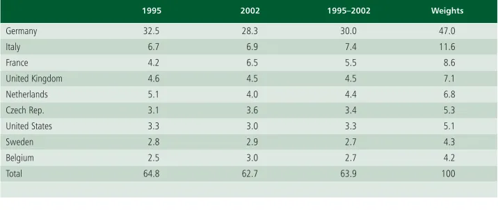
The short-term dynamics of the volume of Polish exports depends on the demand factors, namely foreign demand and price competitiveness of Polish exports on the foreign markets (see eq. 6). The foreign variables are represented by a weighted sum of the foreign output, foreign GDP deflators and the bilateral exchange rates, where weights are proportional to the respective counties’ share in the Polish foreign trade (see Table 1). The estimation results were as follows:

, (31)

where ectXis the error correction term, i.e. the difference between the actual and fitted values in the relationship (30). Short-run demand elasticity of exports is moderate and amounts to 1.70. The statistical properties of the model (31) seem to be plausible, namely: R2=0.63, LM(4)=2.6 [p=0.62] and JB(2)=1.44 [p=0.49].

The import volume, both in the long and short-term horizons, depends solely on the demand factors, i.e. the ratio of import to domestic prices and the level of the domestic activity (see equation 7). After a log-linearisation of the equation (7) the Hansen-Phillips procedure was applied. The results:

(32)

imply that the elasticity of substitution equals β1=0.85. The addition of a trend function into the group of the independent variables was motivated by the same phenomena as in the case of equation (30). The residual analysis, namely ADF=-2.68 (p=0.01) and LC=0.27 (p=0.20), demonstrate that the relationship (32) is cointegrating one.

The short-term dynamics of the volume of imports:

, (33)

5Lowercase letters stand for the logarithms of capital letters, e.g. y = ln(Y). The numbers in the parentheses denote standard deviations of the estimated coefficients.

Table 1

Countries’ share in the Polish foreign trade (%)

1995 2002 1995–2002 Weights

Germany 32.5 28.3 30.0 47.0

Italy 6.7 6.9 7.4 11.6

France 4.2 6.5 5.5 8.6

United Kingdom 4.6 4.5 4.5 7.1

Netherlands 5.1 4.0 4.4 6.8

Czech Rep. 3.1 3.6 3.4 5.3

United States 3.3 3.0 3.3 5.1

Sweden 2.8 2.9 2.7 4.3

Belgium 2.5 3.0 2.7 4.2

Total 64.8 62.7 63.9 100

2

Three inputs of the fundamental equilibrium exchange rate model

indicate, that the demand elasticity is moderate and amounts to 1.74. Statistical properties of the model (33), namely R2=0.67, LM(4)=8.7 [p=0.07] and JB(2)=0.23 [p=0.89], are acceptable.

2.1.2. Export and import prices of goods and services

The relationships (12) and (13) specify export and import prices which are the weighted average of the domestic and foreign prices. As there are sound economic reasons that in the system of the four variables:

(34)

all price indices may be endogenous6_{and there could be more than one cointegrating vector}7_{, the}

Johansen procedure was chosen. Firstly, the optimum lag of the unrestricted VAR was tested. According to the Akaike, Schwarz and Hannan-Quinn information criteria, four lags should be included in the model. Then the number of cointegrating vectors was investigated on the basis of the Johansen’s (1991) trace and maximum eigenvalue tests. The results, which are presented in Table 2, indicate that there are two cointegrating vectors, which have been interpreted in terms of the relationships (12) and (13).

Even though the restrictions on the cointegrating vectors that derive from the equations (12) and (13) were rejected by the data, the values of estimated elasticities:

(35)

(36)

are in line with the economic intuition that Poland, as a small open economy, is in about 80% a price taker country.

The short-term dynamics of the transaction prices was estimated independently within the error correction framework. In both equations, constant terms were excluded and homogeneity restrictions were imposed. The results were as follows:

(37)

. (38)

Statistical properties of both models, i.e. R2=0.64, LM(4)=13.9 [p=0.01], JB(2)=1.1 [p=0.58] for the equation (37) and R2=0.66, LM(4)=14.5 [p=0.01], JB(2)=3.6 [p=0.16] for the relationship (38), seem to be acceptable, despite the occurrence of the residual autocorrelation.

pX pM p (p s)

*₋

[

]

Table 2

Cointegration trace test

Zero hypothesis Trace test Probability Max. Eigenvalue test Probability

r=0 75.3 0.00 37.0 0.00

r≤1 38.3 0.00 28.4 0.00

r≤2 9.9 0.29 8.6 0.32

r≤3 1.3 0.26 1.3 0.26

Source: own calculations.

6Import and export prices are endogenous according to the equations (12) and (13). If pass-through is different from null, then domestic prices react to changes in import prices. Finally, nominal exchange rate component in expression p*–s

may be dependent on terms of trade or domestic price.

2

2.1.3. Simulations

On the basis of the presented model an impact of the domestic as well as foreign demand and the real exchange rate on the net exports and the trade balance has been calculated. This point discusses the results of those simulations.

First, let us focus on the effects of a rise in the domestic demand by 1% of GDP, under the assumption that the levels of all other exogenous variables remain unchanged. This expansion of the domestic demand increases the output and, according to the equation (33), leads to higher volume of imports. The total effect on the output is less than one-to-one, as the net export deteriorates (see equations 3 and 4). As the short-term demand elasticity of imports is 1.74 (see equation 33) and the imports share in GDP amounts to 37.4%8_{, it can be calculated that a cyclical}

rise in the domestic demand by 1% of GDP leads to immediate increases in the output and imports by 0.61% and 1.06%9_{, respectively. This translates into a decrease in the net exports by 0.39% of}

GDP. The impact of this shock on the trade balance is negative and amounts to 0.44% of GDP.

The second impulse that was introduced to the model was defined as a cyclical expansion of the foreign output by 1%. This shock increases domestic exports by 1.7% (see equation 31). As the export share in GDP is 35.9%10, it can be calculated that a cyclical rise in foreign output by 1% leads to increases in domestic output and imports by 0.37% and 0.64%, respectively. This time, net exports improve by 0.37% of GDP. All the changes are instantaneous.

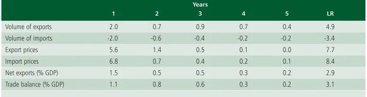
Finally, the response of the model to the exchange rate shock, defined as a 10% permanent real depreciation of the zloty, was analysed. Within a system made up of identities (3), (4), (9), (10), (11) and behavioural equations (31), (33), (37), (38) the impact of such impulse on export and import prices and volumes can be calculated. The results presented in Table 3 indicate that in five years’ horizon the net exports improve by about 2.9% of GDP, where the two thirds of the adjustment occurs in the two initial years.

2.2. Internal equilibrium

The internal equilibrium is defined to occur when the actual output equals its potential level (see equation 1). In this sense, internal balance implies that the goods markets clear11. In order to quantify the internal disequilibrium it is necessary to assess the unobservable level of potential output. The problem is not trivial, as there is no unique and commonly accepted method of measuring this quantity. In practice, there exist a large number of various approaches to calculate the level of potential output (see Table 4). It appears, however, that the different methods lead to generally unlike results. The correlation of output gaps is low, the methods imply various turning points and the

8NBP estimates for 2004.

9A perceptive reader may notice that 1.06=1.74*0.61.

10NBP estimates for 2004.

11Some authors (e.g. Williamson 1994) define internal equilibrium in terms of the labour market, namely if the actual unemployment equals the NAIRU (non-accelerating rate of unemployment).

Table 3

An impact of 10% permanent depreciation of the RER on foreign trade Years

1 2 3 4 5 LR

Volume of exports 2.0 0.7 0.9 0.7 0.4 4.9

Volume of imports -2.0 -0.6 -0.4 -0.2 -0.2 -3.4

Export prices 5.6 1.4 0.5 0.1 0.0 7.7

Import prices 6.8 0.7 0.4 0.2 0.1 8.4

Net exports (% GDP) 1.5 0.5 0.5 0.3 0.2 2.9

Trade balance (% GDP) 1.1 0.8 0.6 0.3 0.2 3.1

2

Three inputs of the fundamental equilibrium exchange rate model

volatility of output gaps is dissimilar. This was illustrated by Chagny and Dopke (2001), who compared the potential output for the euro area economy calculated on the basis of different methods.

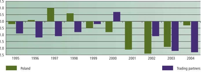
In this paper the output gap data for Poland and for foreign countries were calculated on the basis of the Cobb-Douglas production function. In comparison to other methods, the production function approach seems to be the most intuitive. Moreover, the main advantages of this method are its strong economic foundations. The data of the output gap for Poland were taken from the study by Gradzewicz and Kolasa (2005) and for the Polish main trading partners, which are listed in Table 1, from the OECD database. The values for the foreign countries were estimated also on the basis of the Cobb-Douglas production function, according to the methodology presented in Giorno et al.(1995) and can be found in the OECD Outlook No. 76 (2004).

2.3. External equilibrium

The most controversial part in the presented model refers to the level of target current account balance (TCAB). It appears that the estimates of the fundamental equilibrium exchange rate are very sensitive with respect to the value of the TCAB. This is especially true for relatively closed economies, where even small changes of the current account balance require substantial exchange rate adjustments. This controversy also stems from the fact that there is no generally accepted economic theory that could be a guideline in the calculations of the TCAB level. This point briefly discusses different approaches to calculating a target current account level.

The first method to assess a current account dynamics is based on the intertemporal approach. The initial theoretical models, however, have failed to reflect the observed current account changes. These models predict excessive current account changes in response to various shocks. For example, Obstfeld and Rogoff (1996) presented a simple model that in the steady-state produced the trade surplus equal

Tabela 4

Methods to estimate the output gap

• Peak-to-peak; linear detrending; robust detrending; phase average detrending; • Hodrick-Prescott filter; Beverige-Nelson decomposition; unobservable component

or band-pass filter

• Survey data

• Okun’s law; production function approaches, long-run restriction models (SVAR)

• Multivariate Beverige Nelson decomposition, multivariate Hodrick-Prescott filter, multivariate unobservable component method

Non-Structural methods

Direct measures

Structural methods

Multivariate methods

Source: adapted from Chagny and Dopke (2001).

Poland Trading partners

-2.5 -2.0 -1.5 -1.0 -0.5 0.0 0.5 1.0 1.5

2004 2003

2002 2001

2000 1999 1998

1997 1996 1995

Figure 2

Output gap in Poland and in its main trading partners

2

to 45% of GDP and the foreign debt stabilised at a level that was equal to 15-year value of the GDP. If this basic model, however, is extended for default risk, costs of adjustment or non-Ricardian consumers, etc. then it may generate the results that are closer to reality. Bussiere, Fratzscher and Muller (2004), for instance, developed a model with two types of consumers: the non-Ricardians, who consume their entire disposable income, and the Ricardians, who maximise the utility function with habit formations. The solution of this theoretical model leads to a parsimonious specification, where the current account balance depends on its lagged values and variables such as relative income, relative investment and fiscal balance. The authors claim, that the estimation results provide credible explanation of the past changes in the current account balances for 33 countries included in the sample. In case of Poland, the authors have found that in 2002 the current account balance should amount to -2.4 or -5.2% of GDP, depending on the method of estimation. It should be added here, that even though the intertemporal approach models seem to be theoretically plausible, their empirical properties still require further investigation.

The second approach, which was proposed by Debelle and Faruquee (1998), was christened “macroeconomic balance approach”. In compliance with this method the current account balance is regressed in respect to the long-term determinants of savings and investments such as the stage of economic development, demographics and macroeconomic policies. The theoretical value of this regression, conditional on the assumption that the explanatory variables are in their medium-term equilibrium, is supposed to equal the level of the TCAB. In case of the Central and Eastern European countries, the macroeconomic balance approach was applied by Doisy and Herve (2001). The authors found that the level of the TCAB for Poland in 1998 amounted to -2.6 or -3.2% of GDP, depending on the assumption related to the medium-term level of the budget deficit. The main disadvantage of the macroeconomic balance approach is that in empirical applications, a high share of the TCAB variability across countries is justified not by explanatory variables, but by the country specific constants included in the panel regressions.

The third approach to calculating the target current account balance is based on the solvency criterion. This method defines the TCAB as the value of the current account balance that would stabilise the net foreign debt at its steady-state value. That implies that the TCAB calculations require an assessment of the steady-state level of the net foreign debt. Ades and Kaune (1997), for instance, calibrated “default risk” model, which had been proposed by Obstfeld and Rogoff (1996), in order to calculate the maximum accessible net foreign debt for a group of developing countries. They computed that Polish net foreign debt should not exceed 55.4% of GDP. In other case it would be more profitable for Poland to default than to service this debt. The more recent calculations of the European Commission (European Economy, 2002, p. 127), which are based on the panel regression of the foreign debt on the level of GDP per capita and the degree of openness, indicate that a theoretical value of Polish debt amounts to 39% of GDP. This is not contradictory to the results presented by Pattillo et al.(2002) who estimated that for developing countries, the debt level exceeding 35–40% of GDP has a negative impact on the GDP growth. Taking the above considerations into account, the assumption that the actual value of the Polish net foreign debt, which at the end of 2003 amounted to 42.3% of GDP12_{, is in the steady-state seems realistic.}

If a country maintains its ratio of the net foreign debt (NFD) to GDP at a constant level, this does not imply that the current account balance is null. According to Milesi-Feretti and Razin (1996), the level of the current account balance that stabilises this ratio is equal to:

.13 (39)

If the expression in brackets in the equation (39) is plausibly assumed to equal 7%, one could calculate that the current account deficit that would stabilise the net foreign debt of Poland at the actual level equals to 3.0% of GDP. This value is set as the level of the TCABin further calculations. It can be noted here that this level is not inconsistent with the results of the studies based on the intertemporal and macroeconomic balance approaches.

CAB Y

NFD Y

S t

Y t

NFD Y

Q t

Y t

P t

N N

N

N

= − ∂

∂ + ∂ ∂ = −

∂

∂ + ∂∂ + ∂ ∂

( ln( ) ln( )) ( ln( ) ln( ) ln( ))

*

12On the basis of international investment position statistics, www.nbp.pl.

2

Three inputs of the fundamental equilibrium exchange rate model

Finally, let us assume the steady-state values for the balances on income and transfers (see equations 8 and 9). If the nominal interest rate on the net foreign debt (i) equals to 5%, then the medium-term value of the balance on income equals to -2.2% of GDP, according to the relationship:

. (40)

In case of balance on transfers, taking the inflows of the EU funds enlarged by transfers of Poles working abroad into account, it is possible to assume that its medium-term level equals to 3.5% of GDP (cf. Centrum Europejskie Natolin, 2003, p. 39). Consequently, according to (9) we can calculate, that the target level of the trade balance (TCAB_TB) amounts to -4.3% of GDP.

3

3

The results

The previous sections have presented the foreign trade model and discussed issues concerning the internal and external equilibria. These three issues combined together allow us to calculate the level of the fundamental equilibrium exchange rate for the zloty. It should be stressed that the plausibility of the final results depends on the credibility of these three inputs.

This section demonstrates the method of estimating the fundamental equilibrium exchange rate. Additionally, the sensitivity analysis of the final results is performed.

3.1. The level of the zloty’s fundamental equilibrium exchange rate

Calculations of the fundamental equilibrium levels of the exchange rate and the domestic demand are performed in two steps. Firstly, one must calculate the values of the trade balance and the net exports if output gaps were null and past changes of the real exchange rate materialised. These levels, which are referred to as the adjusted trade balance (ACAB_TB) and the adjusted net exports (ANT), can be calculated according to the following formulas:

(41)

, (42)

where and :

, (43)

, . (44)

Expressions and denote materialised impact of i-th period lagged real exchange rate change ( ) on the trade balance and the net exports, respectively. Consequently, one can calculate that the adjusted output gap (AGAP) equals to:

, (45)

where the GAPis the difference between the actual and potential output:

. (46)

The results, which are presented in Table 5, indicate that in 2004 the ACAB_TBwas lower than the CAB_TBby 0.2% of GDP and the difference between AGAPand GAPamounted to -0.3% of GDP. This difference is the sum of the two opposite effects. On the one hand, low foreign demand (see Figure 2) indicates that the adjusted values should be higher than the actual ones. On the other, the immaterialised effects of the zloty’s appreciation, which occurred in 2004, translate into a fall of ACAB_TBand AGAP.

In the second stage, it is required to estimate the extent of the domestic demand and the real exchange rate changes necessary to equalise the adjusted values of the trade balance and the output gap to their target levels. In section 2 it has been shown how the control variables, i.e. the

GAP= −Y Y

AGAP=DD+ANT− =Y GAP+ANT−NT

∆qt i−

ϑi∆qt i−

θi∆qt i−

ϑ= ϑ

→∞ lim i i ϑi t t j j i _NT q = ∂ ∂ − =

∑

θ= θ

→∞ lim i i θi t t j j i CAB TB q = ∂ ∂ − =

∑

ANT NT NT

y y y q

t t

t

t

t t i t i

i = + ∂ ∂ − + − − = ∞

∑

( ) (ϑ ϑ ∆)

0

ACAB TB CAB TB CAB TB

y y y q

t t

t

t

t t i t i

i

_ ₌ _ _{+ ∂} __* ( * *) ( )

∂ − + − −

= ∞

∑

3

The results

domestic demand and the real exchange rate, influence the current account balance and the domestic output. It has been shown, that a rise in the domestic demand by 1% of GDP leads to an increase of the GAPby 0.61% of GDP and to a deterioration of the CAB_TBby 0.44% of GDP. The impact of the real exchange changes has been presented in Table 3. Thus, it can be calculated, that:

(47)

. (48)

As the adjusted values of the output gap and the trade balance in the equilibrium are equal to their target levels, the required changes amount to:

(49)

(50)

On the basis of the expressions (47)–(50) on can see that the deviations of the control variables from its fundamental equilibrium levels are the solution of the system:

, (51)

which is given by:

. (52)

Substitution of the respective values from Table 5 into the expression (52):

(53)

leads to the final results, which imply that in the forth quarter of 2004 the quarterly average real effective exchange rate of the zloty was undervalued by 4.3% and the domestic demand was subdued by 3.1% of GDP14_{. As this result is conditional on a set of assumptions, it should be}

interpreted cautiously. This issue is discussed below.

3.2. Sensitivity analysis

The results in the previous point indicate that in the forth quarter of 2004 the zloty’s rate was undervalued by 4.3%. It should be emphasised, however, that the plausibility of this result depends on the plausibility of three inputs that were outlined in the section 2. It can be said that the estimated fundamental equilibrium exchange rate is conditional on the assumptions concerning the level of the output gaps at home and abroad, and the target trade balance. This point discusses how these assumptions affect the final result.

( ) / . . . . . . . .

DD DD Y q q FEER FEER − −     

 =_−0 98_{1 39} −_{−1 93}0 94_{ −}_0 6_{2 7}_= _{4 3}3 1_

( ) / . .

. .

/

( _ _ ) /

DD DD Y q q

AGAP Y TCAB TB ACAB TB Y

FEER FEER N − −     

 =_−0 98_{1 39} −₋0 94_{1 93}__ − ₋ _

− −    = − − −     − −       AGAP Y TCAB TB ACAB TB Y

DD DD Y q q N FEER FEER / ( _ _ ) / . . . . ( ) /

0 61 0 29

0 44 0 31

∆CAB TB_ =TCAB TB_ −ACAB TB_

∆AGAP= −AGAP

∆

(

)

(

)

∆

(

)

(

)

Table 5

Balance on goods and services and output gap in Poland in 2004

CAB_NT Domestic output gap

(%GDP) (%GDP)

Actual value -1.4 -0.3

Adjusted value -1.6 -0.6

Adjustment due to: foreign output gap 0.9 0.9

past changes of real exchange rate -1.2 -1.2

Target value -4.3 0.0

Source: NBP, own calculations.

3

3.2.1. Foreign output gap

First, it is investigated how the foreign output gap assumptions affect the final results. An impact of an increase of the assumed level of the foreign output gap by 1% of GDP on the final results is calculated. The analysis is conducted by comparing the solutions of the baseline scenario to the scenario with higher external output gap, which is referred to as scenario 1. In the presented model, this change in assumptions influences the level of the adjusted values of domestic output gap and trade balance. The calculated multipliers indicate that the AGAP and the ACAB_TB would be lower by 0.36 and 0.37% of GDP, respectively. According to the equation (52) the final results change by:

, (54)

where and are the fundamental values of the domestic demand and the real

exchange rate in scenario 1. As a result, if the true foreign output gap was higher than the baseline value by 1% of GDP, the fundamental equilibrium exchange rate would be 1.2% weaker. The relationship between the assumed level of foreign output gap and the scale of the zloty’s misalignment in the forth quarter of 2004 is presented in Figure 3. It can be seen there, that if the true foreign output gap in 2004 was null15_{, in the fourth quarter of 2004 the zloty was}

undervalued by 1.3%.

3.2.2. Domestic output gap

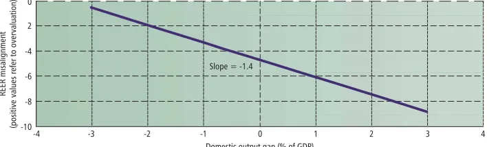
The second analysis investigates how the final results respond to an increase in the assumed level of the domestic output gap by 1% of GDP. The analysis is conducted by comparing the solutions of the baseline scenario to the scenario with higher domestic output gap, which we refer to as scenario 2. In the model, this change in assumptions would increase the adjusted value of the domestic output gap by 1% of GDP. In line with the equation (52) the final results change by:

, (55)

where and are fundamental values in scenario 2. This means that if the true domestic output gap was higher than the baseline value by 1% of GDP, the fundamental equilibrium exchange rate would be 1.4% stronger and the domestic demand should be lower by 1.0% of GDP. The relationship between the assumed level of domestic output gap and the scale of the zloty’s misalignment in the forth quarter of 2004 is presented in Figure 4. It shows that if the true value of the domestic output gap in 2004 was null, in the fourth quarter of 2004 the zloty was undervalued by 4.7%.

qFEER 2 DDFEER 2 ( ) / . . . . . .

DD DD Y q q

FEER FEER

FEER FEER

2

2

0 98 0 94

1 39 1 93 1 0 0 98 1 39 − −       =_− −₋ _− _=_− _ qFEER 1 DDFEER 1 ( ) / . . . . . . . .

DD DD Y q q

FEER FEER

FEER FEER

1

1

0 98 0 94

1 39 1 93 0 36 0 37 0 0 1 2 − −       =_− −₋ _ _=_− _

15Author doubts that this assumption is true.

-5 -4 -3 -2 -1 0 1 2

-3 -2 -1 0 1 2 3

Foreign output gap (% of foreign GDP) Slope = 1.2

REER misalignment

(positive values refer to overvaluation)

Figure 3

Sensitivity of the zloty’s misalignment with respect to the assumed level of the foreign output gap

3

The results

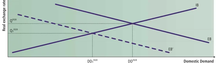
The intuition of the relationship between the assumed level of the domestic output gap and the value of the fundamental real exchange rate is presented in Figure 5. In response to an increase in the assumed level of the domestic output gap the internal balance locus IB moves leftward to the IB’ position, as lower potential output requires lower domestic demand to meet the internal equilibrium condition (see equations 1 and 3). The external equilibrium locus remains unchanged. In the new equilibrium the domestic demand is lower by ( ) and the real exchange

rate appreciates by ( ).

3.2.3. Target level of balance on trade and services

The third analysis investigates how the final results respond to an increase in the assumed level of the target trade balance by 1% of GDP. The analysis is conducted by comparing the solutions of the baseline scenario to the scenario with higher level of the TCAB_TB, which is referred to as scenario 3. This higher value of the TCAB_TB may result from higher level of the target current account balance or lower assumptions concerning the balance on transfers. In this sense this analysis seems very interesting as it answers the question how foreign transfers influence the fundamental equilibrium values of the domestic demand and the real exchange rate.

The change in the supposed level of the TCAB_TB by 1% of GDP affects the final results according to the equation (52):

, (56)

where and are the fundamental values of the respective variables in scenario 3. This means that a decrease in the foreign transfers by 1% of GDP leads to the depreciation of the

qFEERR 3 DDFEER 3 ( ) / . . . . . .

DD DD Y q q

FEER FEER

FEER FEER

3

3

0 98 0 94

1 39 1 93 0 1 0 94 1 93 − −       =₋ −₋       = − −    

QFEER QFEER

2 −

DDFEER₋DDFEER

2 -10 -8 -6 -4 2 0

-4 -3 -2 -1 0 1 2 3 4

Domestic output gap (% of GDP) Slope = -1.4

REER misalignment

(positive values refer to overvaluation)

Figure 4

Sensitivity of the zloty’s misalignment with respect to the assumed level of the domestic output gap

Source: own calculations.

Domestic Demand

Real exchange rate

DDFEER

DD2FEER

IB IB’

EB Q2FEER

QFEER

Figure 5

The domestic demand and the real exchange rate in response to an increase in the assumed level of domestic output gap

3

fundamental equilibrium exchange rate by 1.9%. Moreover, domestic absorption should be lower by 0.9% of GDP. The relationship between the assumed level of the foreign transfers16and the scale of the zloty’s misalignment in the forth quarter of 2004 is presented in Figure 6. It can be seen there, for instance, that if the medium-term level of the balance on transfers is equal to 2% of GDP, then in the fourth quarter of 2004 the zloty was undervalued by 1.4%.

The intuition behind the relationship between the level of the balance on transfers and the value of the fundamental real exchange rate is presented in Figure 7. In response to an increase in the TCAB_TB the external balance locus EB moves downward to EB’ position, as higher trade balance requires currency depreciation to meet the external equilibrium condition (see equations 8, 9 and 25). The internal equilibrium locus remains unchanged. In a new equilibrium the domestic demand is lower by ( ) and the real exchange rate depreciates by (QFEER₋QFEER).

3

DDFEER₋DDFEER

3

-8 -6 -4 -2 0 2 4

0 1 2 3 4 5

Balance on transfers (% of GDP)

REER misalignment

(positive values refer to overvaluation)

Slope = -1.9

Figure 6

Sensitivity of the zloty’s misalignment with respect to the assumed value of the balance of transfers

Source: own calculations.

Domestic Demand

Real exchange rate

DDFEER

DD3FEER

EB IB

EB’ QFEER

Q3FEER

Figure 7

The domestic demand and the real exchange rate in response an increase in the target level of the balance on goods and services

Source: own calculations.

4

Summary

4

Summary

In May 2004 Poland joined the European Union and in subsequent years it is supposed to enter the European Monetary Union. Common monetary policy offers long-term benefits such as lower risk premium, fall of transaction costs, lower currency risks etc. In the short-term horizon, however, the EMU accession may be a challenge for Polish economy, especially if the conversion rate is set at a misaligned level. This paper attempted to investigate this issue. The partial equilibrium model was proposed. This model was used to calculate the level of the fundamental equilibrium rate of the zloty. The results suggest that in the forth quarter of 2004 the zloty was undervalued by 4.3%. As these results depend on a set of assumptions the sensitivity analysis was performed. It has been found out that in this period, in case of a low net inflow of the EU transfers, the real exchange rate of the zloty was not misaligned.

5

5

References

1. Ades, A. and Kaune, F. (1997): A New Measure of Current Account Sustainability for Developing Countries.Goldman-Sachs Emerging Markets Economic Research.

2. Bayoumi, T. and Faruqee, H. (1998): A Calibrated Model of the Underlying Current Account. In Faruqee H., Isard P., ed.

3. Borowski, J., ed. (2004): A Report on the Costs and Benefits of Poland’s Adoption of the Euro. National Bank of Poland.

4. Bussiere, M., Fratzscher, M. and Muller, G. (2004): Current Account Dynamics in OECD and EU Acceding Countries – an Intertemporal Approach. ECB WP No. 311.

5. Centrum Europejskie Natolin (2003): KorzyÊci i koszty cz∏onkostwa Polski w Unii Europejskiej.

Warsaw.

6. Chagny, O. and Dopke, J. (2001): Measures of the Output Gap in the Euro-Zone: An Empirical Assessment of Selected Methods. Working Paper No. 1053, Kiel Institute of World Economics, Kiel.

7. Clark, P. and MacDonald, R. (1998): Exchange Rates and Economic Fundamentals: A Methodological Comparison of BEERs and FEERs. IMF Working Paper WP/98/67, International Monetary Fund, Washington.

8. Devarajan, S. (1999): Estimates of Real Exchange Rate Misalignment with a Simple General-Equilibrium Model. Chapter VIII in Hinkle L., Montiel P., eds.

9. Debelle, G. and Faruqee, H. (1998): Saving-Investment Balances in Industrial Countries: An Empirical Investigation. In Faruqee H., Isard P., ed.

10. Doisy, N. and Herve, K. (2001): The Medium and Long Term Dynamics of the Current Account Positions i the Central and Eastern European Countries: What Are the Implications for their Accession to the European Union and the Euro Area? Preliminary version.

11. Driver, R. and Wren-Lewis, S. (1998): Real Exchange Rates for the Year 2000. Institute for International Economics, Washington.

12. European Economy No. 3/2002: Public finances in EMU. European Commission,

Directorate-General for Economic and Financial Affairs.

13. Faruqee, H. and Isard, P. (1998):Exchange Rate Assessment: Extension of the Macroeconomic Balance Approach. IMF Occasional Paper 167, International Monetary Fund, Washington.

14. Faruqee, H., Isard, P., Kincaid, R. and Fetherston, M. (2001): Methodology for Current Account and Exchange Rate Assessments. IMF Occasional Paper 209, International Monetary Fund, Washington.

15. Frankel, J. and Froot, K. (1986): The Dollar as a Speculative Bubble: A Tale of Fundamentalists and Chartists. NBER Working Paper No. 1854, National Bureau of Economic Research, Cambridge.

16. Frenkel, J. (1976): A Monetary Approach to the Exchange Rate: Doctrinal Aspects and Empirical Evidence. „Scandinavian Journal of Economics” vol. 78, p. 200–224.

5

References

18. Goldstein, M. and Khan, M. (19850): Income and price effects in foreign trade. Chapter XX

in Jones R., Kenen P. (eds.): Handbook of International Economics. Vol. II, Elsevier Science Publishers B.V.

19. Gradzewicz, M. and Kolasa, M. (2005): Estimating the output gap in the Polish economy: the VECM approach. IFC Bulletin No. 20.

20. Grossman, G. and Rogoff, K., eds. (1995): Handbook of International Economics. Vol. III., Elsevier Science Publishers B.V.

21. Hansen, B. (1992): Tests for Parameter Instability in Regressions with I(1) Processes. „Journal of Business and Economic Statistics” vol. 10, s. 321–334.

22. Hansen, B. and Phillips, P. (1990): Statistical Inference in Instrumental Variables Regression with I(1) Processes. „Review of Economic Studies” vol. 57, s. 99–125.

23. Hansen, J. and Roeger, W. (2000): Estimation of Real Exchange Rates. Economic Papers

ECFIN/534/00-EN, Directorate General for Economic and Financial Affairs, European Commission.

24. Hinkle, L. and Montiel, P. (1999): Exchange Rate Misalignment. World Bank Research Publication, Washington.

25. Johansen, S. (1988): Statistical Analysis of Cointegrating Vectors. „Journal of Economic Dynamics and Control” vol. 12, s. 231–254.

26. Johansen, S. (1991): Estimation and Hypothesis Testing of Cointegrating Vectors in Gaussian Vector Autoregression Models. „Econometrica” vol. 59, s.1551–1580.

27. Jones, R. and Kenen, P., eds. (1985): Handbook of International Economics. Vol. I and II, Elsevier Science Publishers B.V.

28. MacDonald, R. (2000): Concepts to Calculate Equilibrium Exchange Rates: An Overview. Discussion Paper 3/00, Deutsche Bundesbank.

29. Meier, C. (2004): Investigating the impact of an appreciation of the euro in a small macroeconometric model of Germany and the euro area. Kiel WP No. 1204.

30. Milesi-Ferretti, G. and Razin, A. (1996): Sustainability of Persistent Current Account Deficits. NBER Working Paper No. 5467, National Bureau of Economic Research, Cambridge.

31. Mroczek, W. and Rubaszek, M. (2003): Determinanty Polskiego Eksportu i Importu. NBP Paper

No. 161, National Bank of Poland, Warsaw.

32. Mroczek, W. and Rubaszek, M. (2004): Development of the trade links between Poland and the European Union in the years 1992–2002. NBP Paper No. 30, National Bank of Poland, Warsaw.

33. NBH (2002): Adopting the euro in Hungary: expected benefits, costs and timing. NBH Occasional Paper No. 24, National Bank of Hungary, Budapest.

34. Obstfeld, M. and Rogoff, K. (1995): The intertemporal Approach to the Current Account. Chapter 34 in Grossman G., Rogoff K., eds.

35. Obstfeld, M. and Rogoff, K. (1996): Foundations of International Macroeconomics. MIT Press. OECD Economic Outlook No. 76, 2004, OECD, Paris.

36. Pattillo, C., Poirson, H. and Ricci, L. (2002): External Debt and Growth. IMF Working Paper WP/02/69, International Monetary Fund, Washington.

37. Roseberg, M. (1996): Currency Forecasting. IRWIN, Chicago.

38. Rubaszek, M. (2003): Optimal ERM II Central Parity for Polish Zloty. ECB conference „Equilibrium Exchange Rates in Accession Countries: Macroeconomic and Methodological Issues” papers.

5

40. Rubaszek, M. (2004b): Modelowanie optymalnego poziomu realnego efektywnego kursu z∏otego. Zastosowanie koncepcji fundamentalnego kursu równowagi. „Materia∏y i Studia”,

Narodowy Bank Polski, Zeszyt nr 175.

41. Rubaszek, M. (2004c): Porównanie w∏aÊciwoÊci statystycznych ró˝nych estymatorów relacji kointegrujàcej metodà symulacji Monte Carlo (A Monte Carlo comparison of statistical properties of various methods to estimate cointegrating relationship.). Internal research at Warsaw School of Economics.

42. Stein, J. (1995): The Fundamental Determinants of the Real Exchange Rate of the U.S. Dollar Relative to Other G-7 Countries. IMF Working Paper WP/95/81, International Monetary Fund,

Washington.

43. Stockman, A. (1987): The equilibrium Approach to Exchange Rates. „Federal Reserve Bank of Richmond Economic Review” vol. 73 (2), p. 12–30.

44. Williamson, J. (1983): The Exchange Rate System. „Policy Analyses in International Economies”

vol. 5, Institute for International Economics, Washington.

45. Williamson, J. (1994): Estimates of FEER. In Williamson J., ed.