Volume 2007, Article ID 49350,10pages doi:10.1155/2007/49350
Research Article
A Variational Approach to the Modeling of MIMO Systems
A. Jraifi1, 2and E. H. Saidi1, 2
1Groupe Canal, Radio & Propagation, Lab/UFR-PHE, Facult´e des Sciences, Rabat, Morocco
2Virtual African Centre for Basic Science and Technology (VACBT), Focal Point Lab/UFR-PHE, Faculty of Sciences, Rabat, Morocco
Received 17 February 2006; Revised 18 June 2006; Accepted 26 March 2007
Recommended by Thushara Abhayapala
Motivated by the study of the optimization of the quality of service for multiple input multiple output (MIMO) systems in 3G (third generation), we develop a method for modeling MIMO channelH. This method, which uses a statistical approach, is based on a variational form of the usual channel equation. The proposed equation is given byδ2= δR|H|δE+δR|(δH)|Ewith scalar variableδ= δR. Minimum distanceδminof received vectors|Ris used as the random variable to model MIMO channel. This variable is of crucial importance for the performance of the transmission system as it captures the degree of interference between neighbors vectors. Then, we use this approach to compute numerically the total probability of errors with respect to signal-to-noise ratio (SNR) and then predict the numbers of antennas. By fixing SNR variable to a specific value, we extract informations on the optimal numbers of MIMO antennas.
Copyright © 2007 A. Jraifi and E. H. Saidi. This is an open access article distributed under the Creative Commons Attribution License, which permits unrestricted use, distribution, and reproduction in any medium, provided the original work is properly cited.
1. INTRODUCTION
Digital communication of the third generation (3G) using multi-input multi-output (MIMO) is one of the important techniques used to exploit the spatial diversity in a rich scat-tering environment [1]. This revival interest in MIMO is pri-marily dictated by the objective of improving the network’s quality of service and the operator’s revenues significantly [2]. Due to the great spectral efficiency gain, MIMO systems have known a great interest nowadays and have been defined by IEEE 802.16 [3], for fixed broadband wireless access and 3G partnership project (3GPP) for mobile applications. Us-ing MIMO, it has been shown in [4] that spectral efficiency can be improved significantly in wireless communications in fading environment.
Recall that the main objective of the optimization pro-cess of the MIMO network is to improve the quality of ser-vices for network and to be sure of optimal exploitation of the resources of network efficiency. For instance, an essential shutter in MIMO and which will be discussed in this work is the theoretical determination of the optimal numbersNT andNRof transmitter and receiver antennas respectively. To our knowledge, few studies in literature have been devoted to theoretical approach of MIMO systems. It would be then interesting to deeper this issue.
To study MIMO system, we will use Rayleigh model as it is the most widely used method for indoor and urban
channels [5]. When the bandwidth is narrow (flat fading)
[6], our system can be modeled byNR∗NT random
ma-trixH. The receivedNR-vector|R, describing received
sig-nals at reception, is related to the transmitted one |E as
|R =H|E+|N, where|Nis the noise vector with
covari-ance matrixσ2I
NR withINR being theNR×NRunit matrix.
When the bandwidth is large as in WCDMA, OFDM (or-thogonal frequency division multiplexing) [7] can be used to divide the large bandwidth into a narrow ones and for each subband, the previous model is used. The gains (Haα) (a = 1,. . .,NR,α = 1,. . .,NT) of channel matrix are sup-posed to be independent identically distributed (iid) and are governed by a circular complex Gaussian random variables with zero mean and unit variance.
In this work, we use differential analysis and borrow ideas from quantum scattering theory [8–10] to develop a new way to deal with MIMO channel. We first derive a scalar equa-tion for modeling MIMO channel; then we study the perfor-mance of MIMO systems for indoor and urban channels by
varying SNR and the antennas numbersNT andNR.
Asso-ciating the MIMO channelH with the random minimum
11000101 Coding Modulation
Mapping 1
. . .
NT
Channel H
1 . . .
NR
Demapping Demodulation
Decoding
11000101
Figure1: Principle of MIMO techniques. Remark thatH plays a quite similar role of the quantum scattering theoryS-matrix of particle physics.
probability of errorsPe=Pe(NT,NR,d0,σ), whered0stands for the minimal distance between transmitted vectors and SNR = −20 log10(σ). We show inSection 4thatPereads in general as follows:
Pe= 1 σ√π
∞
0 e −t2/4σ2
1−1−Γt2/d2 0
NR
NT
dt. (1)
Then we compute numericallyPe with respect to SNR for
fixedNT andd0and varyingNR. By fixing bounds onPefor a given SNR, we study the determination of the theoretical value of the optimal number of antennas. This theoretical analysis, which uses a statistical approach, allows to predict the number of antennas without using long simulations. It permits as well to optimize the conception of MIMO systems and the reduction of the cost of its implementation. Notice by the way that great changes are envisaged to evaluate and migrate to third generation systems (3G). In the fixed net-work, an evolutionary path is envisaged, whereas in the radio interface a revolutionary approach is needed to support high data services [11]. The price to pay for the evolution towards 3G is exorbitant. Research for methods aiming the reduction of the cost of optimization is then essential.
The presentation of this paper is as follows: inSection 2, we give preliminaries on MIMO systems and a brief overview on the third generation (3G) of telecommunications. In
Section 3, we study the performances of MIMO systems deal-ing with 3G. We first develop the modeldeal-ing of MIMO channel
by using the random minimum distance variableδmin. Then
we compute numerically the probability of errorsPein terms of the signal-to-noise ratio variable (SNR). InSection 4we give our conclusion.
2. PRELIMINARIES
We begin by describing briefly the principle of MIMO; then we give an overview on the 3G mobile systems that support circuit and packet oriented.
2.1. Principle of MIMO
From a diagram of a MIMO wireless transmission system (seeFigure 1), a compressed digital source in the form of a binary data stream is fedin to a simplified transmitting block encompassing the functions of error control coding and
mapping to complex modulation symbols (BPSQ, QPSK, M-QAM, etc.). Each separate symbol stream is mapped onto one of the multipleNT antennas. After filtering and ampli-fication, the signals are launched into the wireless channel. At the receiver, the signals are captured byNRantennas and inverse functions are performed to recover the message. For a SISO (single input single output,NT =NR =1) channel,
the capacityC =C(ρ) reads, in terms of SNR (SNR=ρ), as
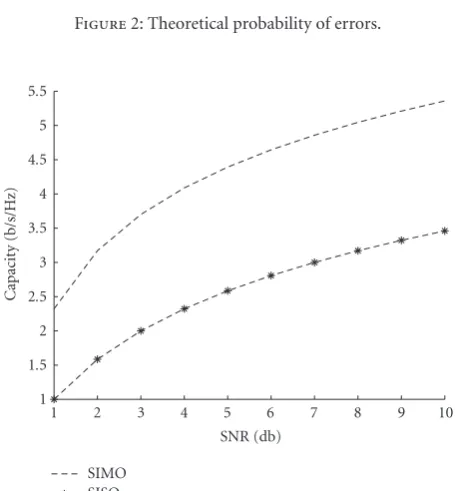
C =log2(1 +ρ) bits/sec/Hz [12]. For a SIMO (single input multiple output,NT =1,NR >1) system, information the-ory can be used to demonstrate that the capacity is given by CNR(ρ)= log2(1 +ρNR2) bits/sec/Hz [13].Figure A.1shows the variation of capacity in terms of SNR for a SISO and SIMO systems.
For a MIMO channel, the capacityC of the system is
given by the following general relation [13]:
CNT,NR(ρ)=log2
det
INR+
ρ
NTHH
+ , (2)
whereNTis the number of transmitters andNRthe number
of receivers. The variableρis the signal-to-noise ratio (SNR),
H is the NR ∗NT channel matrix with adjoint conjugate
H+ and the capacityC is expressed with unit bits/sec/Hz.
Note that this equation is based onNT equal power
uncor-related sources. Foschini and Gans [4] demonstrated that
Table1
(NR,NT) Code rate Modulation Data rate
(1, 1) 3
4 64 QAM 10.8 Mbs
(2, 2) 3
4 64 QAM 14.4 Mbs
(2, 2) 3
4 QPSK 14.4 Mbs
(4, 4) 1
2 8 PSK 21.6 Mbs
Notice moreover that there is a price to pay for improving quality and revenues since additional antenna increases the complexity of the system. This is because of the additional circuits for processing (equalization or interference cance-lation) needed due to dispersing channel conditions result-ing from delay spread of the environment surroundresult-ing the MIMO receiver [4].
2.2. Third generation (3G)
A great demand for a wide range of services (voice, high rate data services, mobile multimedia) is expressed by many users. This leads to a new generation (3G) of mobile sys-tems, IMT-2000, that support circuit and packet-oriented. One of the air-interfaces developed within the frame work of the international Mobile Telecommunications (IMT-2000) is WCDMA (wide code division multiple access) using a di-rect spread technology that spread encoded user data over wider bandwidth (5 MHz), a sequence of pseudo-random units called chips at higher rate (3.84 Mcps) is used.
The basic idea of the 3G system is to integrate all the net-works of 2G whole world in only one network and to asso-ciate it multimedia capacities (high flow for the data). Recall also that CDMA is a modulation and multiple-access using a spread spectrum communication which is used in civil-ian and military communication. It has the ability to combat multipath interference and increase performance systems. Within 3G (third generation partnership project) WCDMA is known as UTRA (universal terrestrial radio access). UTRA is designed to operate in either TDD mode (Time Divi-sion Duplex) or FDD mode (frequency diviDivi-sion duplex). The FDD mode uplink (from user equipment (UE) to the base station (node B)) and downlink transmission (from node B to UE) deploys separated frequency bands. TDD is used when uplink and downlink transmissions are
per-formed within the same frequency band in different time
slots. In terms of capacity and receiver complexity, the down-link is more critical than the updown-link.
WCDMA systems suffer from multiple access
interfer-ence (MAI), because the same frequency band is shared by different users. The desired signal is extracted from its code, while other signals from system users in the home cell and other cells covering the service area appear as additive inter-ference. This received interference is a factor which limits the radio capacity of the system.
3. PERFORMANCE OF MIMO
One of the basic tasks in dealing with MIMO systems is the modeling of the channel generally represented by the ran-domNR∗NTmatrixH. Guided by the analysis of [15] and borrowing ideas from particles scattering theory of quantum mechanics [8–10], we develop, in the first part of this
sec-tion, a way to approachH using the random variableδmin
introduced earlier. In the second part, we use the results of this method to study the performance of MIMO by varying theNRandNTnumbers and the SNR variableσ. To that pur-pose, we first consider the simple caseNR=NT =1,h≡H as a matter to fix the ideas and to make some useful com-parisons with scattering theory and give our equation to ap-proach the channel. Then we focus on special aspects of the channel matricesHwithNR,NT≥2. We give, amongst oth-ers, the general form of the differential scattering equation for MIMO.
3.1. MIMO channels
We start by illustrating ideas on a simple example. This al-lows us to show how results on scattering theory of quan-tum mechanics (QM) can be used to approach MIMO chan-nels. Thus consider a single-input single-output (SISO) sys-tem and focus on the channel of the syssys-tem with matrixh.
Having seen the link between MIMO systems and QM scattering theory, it is interesting to start by recalling some
useful QM tools. An incoming wave e is generally
rep-resented by a Hilbert space vector denoted as |e and
called ket. The outcoming vectorr, belonging to the dual
Hilbert space H, is represented by r| and is called bra. The latter is just the adjoint vector of the ket |r, (r| =
(|r)†). The Hilbert space H is an Euclidean space
en-dowed with the inner product H ×H → C which
asso-ciates to the two vectors f ∈ H∗ andg ∈ H the scalar
f | g. The ket and bra notations satisfy the usual prop-erties of the Hilbert space including linearity and normal-ization; they are very useful in the study of scattering the-ory and their power comes from the fact that they are representation independent; one may work either in the real space or in the Fourier dual and can move from one representation together without difficulty; for details see
Appendix A.2.
Using the input vectorse|and output ones|r, theh matrix reads in particular ash= |re|; but in general like1
h= |re|, e|e =1, (3)
where|rcaptures also the noise vector|nwhich should be thought as an external source. We suppose that the chan-nel gains are identical and independently distributed. There-fore given a transmitted vector|e, which reads explicitly in
M-ary modulation (M =2n) as|b quantum are concerned, one can make a remarkable
corre-spondence between MIMO channelhand quantum
scatter-ing theory of particles. We have, amongst others, the two fol-lowing:
(1) Bits ±1 are in one to one with the quantum states
ψs,m of particles of spins = /2 and spin projection m= ±/2, whereis the Planck constant. This opens an issue to borrow methods used to describe spin par-ticles to approach the channel. Note that the stateψs,m is often denoted as|m= ±1. This vector may be also used to describe the bits vector of BPSK modulation. (2) Equation (3) can be interpreted as just the usualTi f
of quantum scattering theory of spin particless=/2 andm= ±/2 moving in some potential. Within this view one may use QM methods (Green functions) to
computeTi f to approach SISO channel. We will not
develop this issue here; for a review of the QM meth-ods; see, for instance,Appendix A.2and [8–10].
3.1.1. Variational channel equation
Instead of modeling the channel by the typical scattering equation (4), we propose to rather use the following varia-tional one,
|δr =h|δe+δh|e, (6) where the variation vectors are as|δv = |v − |vwith|v
standing for|rand|eand whereδhdescribes a fluctuation of the channel. In the above relation, we have also supposed a constant static noise (|δn =0). Moreover, since|δris an arbitrary vector, one can put the vector equation (6) into the following scalar form:
δ2= δr|h|δe+δr|δh|e, (7)
where nowδ = δr|δr is a random variable that
cap-tures information on the channel and whereδr| = δe|h++
e|(δh+) withh+being theadjoint conjugate ofh. Instead of (6), the channel is now modeled by the above scalar relation. We will turn later on the way this relation can be used in prac-tice; for the moment let us say few words about the extension to MIMO.
3.1.2. MIMO case
The channel matrixHof MIMO systems is described by the
following randomNR∗NT complex matrix which reads in
the bra-ket notations as follows:
H= |RE|, |R = |R − |N, (8)
where|Rmay be thought as anN
R×1 column vector and
E|a row 1×NTone (see (9) below). The matrixHinvolves NT transmitters,NRreceivers, and obeys quite similar rela-tions to SISO; except that in MIMO the previous vectors|r
and|eget now promoted to larger vectors, namely,
|R =
As such, MIMO channel obeys the following generalized
equation|R =H|E+|N, formingNRequations of type
MISO. The differential version of this equation extending (6) reads then as follows:
|δR =H|δE+ (δH)|E. (10)
By taking the norm, we can bring this relation into various forms; in particular,
δ2= δR|H|δE+δR|(δH)|E, (11)
where nowδ2 = δR | δR. Using these differential equa-tions, we will develop, in what follows, the method to model MIMO channel and its optimization. A closed approach has been also considered in [15]. The method involves the two
following ingredients: (a) the minimum distance δmin
be-tween signal vectors |R and|R = |R+|δRat
recep-tion and (b) the optimizarecep-tion of the total probability of
er-rorsPe = Pe(σ) to predict the optimal number of MIMO
antennas.
3.2. Minimum distance as a channel variable
As noted so far, the key point in dealing with MIMO and its
performance is how to model the random channel matrixH.
The latter is in general a non Hermitian rectangular matrix with the unique data is that it satisfies the scattering equa-tionH|E = |R. This lack of information makes the study
of MIMO and in particular itsH matrix not an easy task.
However, there is a clever way to extract information from this matrix without going into involved mathematical anal-ysis. The idea is to optimize the above scattering equation using a variation approach (11) together with special prop-erties of the space of the complex vectors|Eand|R. The idea of the method involves three steps; two of them are sum-marized just below and the third one will be exposed in next
section 3.3.
(1) First use a variational approach which deals with the channel not through the usual scattering equation
H|E = |R, but rather in terms of its variation as shown below:
where we have supposed
HaαδHaα, a=1,. . .,NR,α=1,. . .,NT. (13)
So the above variational scattering equations reduce to
H|δE = |δR.
(2) Take the norm of the simplified vector equation (12) reducing it into a scalar relation δE|H†H|δE =
δR|δRwhereH†H is anNT∗NT square Hermi-tian matrix. Then minimize both sides of the resulting scalar equation leading to the typical relation
δmind0
To see how this works in practice, consider two generic vec-tors|raand|rband their difference|rab ≡ |ra − |rbwith a = b. To make contact with the variational analysis given above, this difference can also be read as|rab = |ra+|δra.
Then compute the minimum of the distance |rabmin in
terms of the transmitted symbols|eaband the channel ma-trixH. We have Therefore, the minimum distanceδminequation (15) is given by
just themth column of theHmatrix.
whereΓ(NR)=(NR−1)!. Moreover, the cumulative distri-bution functionFYm(u) (cdf) associated withYmis
FYm(u)=P
where Γu(p) is the incomplete gamma function defined
as Γu(p) = (1/Γ(p))
u
0 xp−1e−xdx. Then the quantity minm=1,...,NTFYm(u) = P(minm=1,...,NTYm < u) can be
also written, using independence property of Ym’s, as
(minm=1,...,NTFYm(u)) = 1−Πm=1,...,NTP(Ym > u), which,
whereΓu(p) stands for the incomplete gamma function
de-fined above. Thus the cdf for a genericδminreads as follows:
Fδmin
Notice that strictly speaking, the cdf is a function depends on the variablesNT,NR, and the ratioδmin/d0. But later on we will fixNTand look for the optimal values ofNRby studying the variation of the probability of errors Pe with respect to SNR.
3.3. Probability of errors for the minimum distance
We begin this section by noting that given a transmitted
vector |Ei of a packageE including the closed neighbors
|Ei+δEi, one also has the three following vectors at recep-tion.
(a) The basic received noise free vector|Ri =H|Ei. (b) Its closed neighbors; that is, received noise free vectors
|Ri+δRi =H|E+δEwithδH ignored. (c) The basic received noisy vector
|R = |R+|N (23)
with noise vector|N.
With these received vectors we are in position to complete the third stage of the three steps mentioned inSection 3.2. We require the following condition:
N|Nless thanN−δR|N−δR. (24)
This constraint relation is the condition for disregarding
in-terference between the received noisy vector |R and the
received vector |R + δR associated with the transmitted
|Rpatδmin. Then error appears whenever we have confusion between two neighbors vectors
Rq and using the identity
Ep
we get the condition
H tor|δEobeys then the following constraint equation:
|δE =d0exp
iθm0um0
. (28)
Usually, the reason of error comes from the similarity
be-tween the received noisy vector H|E+|N and its
near-est neighborsH|E+δE. The error appears whenever the
norm of the noisy vector is greater than the distance between noise received vector and neighbor noise-free received
vec-tors. Thus error occurs when we haveN ≥ (N−δR),
We can rewrite this relation by remembering that the com-plex random variableυ= N|hm0/
hm0|hm0is a
Gaus-sian complex circular variable with zero mean and variance σ2. Thus, we have Re(eiθυ)> δ
min/2, with probability of er-rors Pe,inf(Re(eiθυ)> δmin/2)=
∞
δmin/2ρυ(x)dxwhereρυ(x)=
(1/σ√π) exp(−x2/σ2). Note that for BPSK constellation, θ takes only one value for a given|E, while for constellation
other than BPSKθtakes more than one value. Using the
ex-pression ofρυ(x), the probability of errors above the lower bound reads then as follows,
Pe,inf
For the upper bound, we should replace Re(eiθυ) > δ min/2 by|υ|> δmin/2. The cdf of|υ|2isF|υ|2(u)=P(|υ|2< u) or
equivalently asF|υ|2(u)=Γu/σ2(1)=1−exp(−u/σ2). For the
upper boundPe,sup(δmin)=P(|υ|2 >(δmin/2)2), the proba-bility of errors can be put into the form
Pe,sup
Ploting the curves of probability of errors Pe,sup and Pe,sup
with respect to δmin, we see that a good compromise
pro-viding quite good results for usual constellation (other than BPSK) is given by
Pe
So, the theoretical total probability of errorsPe can be
ex-pressed as Pe =
whereF(δmin) is the cumulative distribution function ofδmin and Pe(δmin) is the derivative of Pe(δmin).
4. THEORETICAL RESULTS
We first describe the method for evaluatingPe; then we give our numerical results.
4.1. The method
To compute the total probability of errors in terms of signal-to-noise ratio (SNR) variable, that isPe=Pe(SNR), we pro-ceed in steps as follows: first we start from the integral ex-pression ofPe (34), then substituteF(δmin) as in (22) and
Up on fixingd0for a given constellation, this is a real function depending on three parameters as shown below:
Pe=Pe
σ,NT,NR
. (37)
This expression is difficult to compute exactly although it can be simplified a little bit since a priori the numbersNT and NRare two inputs. But here we will deal with them as mod-uli fixed by physical considerations, statistics and desired ser-vices. Next, we adopt a numerical approach to evaluate this quantity. In our computation, we use the following method. (1) We fix once for all the numbers of transmitter
an-tennas asNT = 2 reducing the previousPe moduli
depen-dence to Pe(σ,NR). This is because of electromagnetic in-teraction of antenna elements on small platform and the
ex-pense of multiple down-conversion RF paths [16], the
im-plementation of diversity at user mobile in 3G which cannot support more than two antennas is difficult. Note thatNR
must be greater thanNT, otherwise some power is wasted.
(2) To deal with the two remaining moduliNRandσ, we proceed as follows.
(a) We choose the number of receiver antennasNR into
an interval lying from 3 to 9 (3 ≤ NR ≤ 9). For
each choice ofNR,Pe(σ,NR) becomes a one parameter function which we denote asPe,NR(σ).
(b) Comparing the values ofPe,NR(σ) for each choice of
NR, one gets information on the optimal value ofNR for a given value ofσ.
(3) To extract information on the optimal value of NR,
we draw the parametric curves Pe,NR = Pe,NR(SNR) with
SNR(db) which is equal to−20 log10σ. Recall by the way that SNR(db) = 10 log10(PT/PN) withPT andPN defining, re-spectively, the transmitted power and the power associated with noise at reception. By implementing the expression of the noise covariance matrix, namelyσ2I
NR, and normalizing
the total transmitted power to 1, one gets the above relation between SNR and varianceσ2.
4.2. Numerical results
Below we give our numerical results. These are grouped in the form of figures illustrating the variation of the total prob-ability of errors with respect to SNR.
Notice that as we are interested in 3G, we have adopted the structure of WCDMA physical layer that assumes QPSK modulated data streams assembled into 10 millisecond frames. We recall also that the minimum distanced0between the transmitted symbols in a QPSK modulation is√2.
FromFigure 3, we learn the three following:
(i) For a given SNR and for a desired value of probability of errors, we can determine the number of antennas to in-stall. Choosing a MIMO performance with total probability of errors as
Pe,NR(SNR)<10−6 (38)
at SNR=6 dB, we find that the required number of received antennas is at leastNR=9. As we can see, this number is too high because of the required high performance. Relaxing this requirement by choosing for instancePe,NR(SNR)<10−3we
getNR = 4. The number of antennas at reception strongly
depends then on the precision ofPe,NR(SNR).
(ii) Knowing that the choice of the probability of errors depends on the type of service we want to send on the chan-nel (voice, data, image), we can, by help ofFigure 2, deter-mine the optimal value of the received antennas as shown on
Table 2.
(iii) The same approach may also be used for other tech-niques such as EDGE, HSDPA, and WIMAX using, respec-tively, the modulations 8-PSK, QAM, and QPSK. In these techniques, the same relation for the probability of errors
(36) is valid except that now we have to vary the
mini-mum inter-distance d0 between transmitter signal vectors.
For instance, for QPSK,d0 =
Figure2: Theoretical probability of errors.
10
Figure3: Variation of capacityCwith respect to SNR. Upper curve describes SIMO and lower one is for SISO.
Table2
the usual channel vector equation |R = H|E+|N, we have proposed a variational relation for approaching MIMO channel; see (7)–(11). This is a scalar equation involving the
minimum distance δmin as a random variable. Restricting
our analysis to the caseδH 0, we have shown that much
on the MIMO channel is encoded in the minimum distance δmin = min(
δR|δR) between received vectors|Rand
|R+δR.
Moreover, we have considered the theoretical determina-tion of the number of antennas in MIMO systems combined to the third generation. This approach, which agrees with the study of [15], is important because it is easy to implement for predicting the theoretical optimal number of antennas.
Furthermore, if one succeeds to integrate some system parameters into the above theoretical result, this approach could also be used for other applications. Digital modula-tion such as QPSK (quadrature phase shift keying) and QAM (quadrature amplitude modulation) are used for many com-munication systems 3G, WIFI, HSDPA, and WIMAX. The probability of errors for constellations using HSDPA and
WIMAX (QAM, QPSK) is given by the same equation (36).
This means that the same analysis and quite similar results can be applied for other new technologies such as HSDPA and WIMAX technologies.
APPENDIX
We give two Appendices A.1andA.2: inAppendix A.1 we
give figures describing the variation of capacityC with re-spect to signal-to-noise ration (SNR). InAppendix A.2, we describe briefly the link between MIMO channel and wave scattering theory of quantum mechanics.
A.1. MIMO capacity
We give two figures; Figure A.1 illustrates the variation of
MIMO (SISO and SIMO) capacity C with respect to SNR
andFigure A.2illustrates its average for various numbersNR of received antennas.
A.2. General wave scattering theory
In this appendix Section, we show briefly how standard methods of scattering theory can be used to study MIMO channel. Here we exhibit rapidly the parallel between the channel equation of radio propagation and the so-called Born series of scattering theory of quantum physics; for refer-ences on applications of methods of scattering theory see for instance [17–19]. For other applications of methods of math-ematical physics, such as large random matrices and maxi-mum entropy principle, see Wigner proposal [20,21]. Notice that as the subject of scattering theory is very huge, we will content ourselves here to expose the basic idea by giving the main lines of this correspondence. We hope to come back in a future occasion to give more details on how methods and results of scattering theory could be used in MIMO engineer-ing.
10 9 8 7 6 5 4 3 2 1
SNR (db) 5
10 15 20 25 30 35
Capacit
y
(b/s/Hz)
MIMO channel
NR=10 NR=9 NR=8
NR=7 NR=6 NR=5
FigureA.1: Average capacity for MIMO systems. Curve in bottom is forNR=5 and top one forNR=10.
Incidental waves
Scattered wave
Obstacles
Scattered waves
FigureA.2: Illustration of scattered phenomenon.
Link between channel equation and Born series
For readers who are not familiar with scattering theory and before going into technical details, we begin by noting that the usual MIMO channel equation (4),
|s =h|e+|n, (A.1)
of radio propagation model looks like the following basic equation of wave scattering theory:
Ψscat
=Iid+G0V+G0V G0V+G0V G0V G0V . . .Ψinc
. (A.2)
Green distribution describing the line of sight (free space) propagation; see Figure A.2for illustration. Notice that the objects|φ(φ|) withφ = Ψinc,Ψscat, which in the context of radio propagation should be thought as|φ = |e,|s,|n, are standard tools currently used in quantum mechanics. The objects|φandφ|are known as ket and bra vector waves (Dirac formalism); they constitute a clever way to study wave scattering and allow to avoid the usual complexity of integral computation.
To fix the ideas, let us give the link between the usual space wave functionφ(x,y,z) and Dirac formalism. This is obtained by help of the resolution formula of the identity op-eratorIid. For one dimensional waves, for instance,φ(x) the resolution of the identityIidreads as follows:
Iid=
ρxdx, ρx= |xx|, (A.3)
whereρxis the projector on the wave positionx, we have
|φ =Iid|φ =
φ(x)|xdx, x|φ. (A.4)
With these conventions of notations, the usual Dirac-delta function
reads in real space as follows:
δx1−x2
=x2|x1
. (A.6)
Notice also that by using a normalized incidental wave|e, which reads in real 3-dimensional coordinate space as:
R3d
3xe(x,y,z)2=1, x=(x,y,z) (A.7)
or equivalently in Dirac formalism just like
e|e =1. (A.8)
Then substituting the noise vector|n = |n ×1 by
|ne|e =|ne||e, (A.9)
we can rewrite (A.1) into the following equivalent form:
|s =h|e (A.10)
(1) The matrixhof the MIMO radio propagation
chan-nel is equal to the Born series of scattering theory
h=Iid+G0V+G0V G0V+G0V G0V G0V . . .
. (A.12)
Under an assumption of the nature of the propagation envi-ronment associated with a hypothesis on the eigenvalues of theG0V, the matrixhcan be read, for smallV’s, also as
h= 1
1−G0V
, (A.13)
whereG0is the Green function for line of sight andV poten-tial barrier models the environment.
(2) From (A.2), one learns as well that the scattered wave
|Ψscathas the remarkable structure
Ψscat
line of sight (LOS), one diffusion, two diffusions,
(A.15)
and so on.
ACKNOWLEDGMENTS
The authors would like to thank Gilles Burel for discussions. This work is supported by Protars III D12/25/CNR.
REFERENCES
[1] D. J. Love, R. W. Heath Jr., W. Santipach, and M. L. Honig, “What is the value of limited feedback for MIMO channels?”
IEEE Communications Magazine, vol. 42, no. 10, pp. 54–59, 2004.
[2] D. Gesbert, M. Shafi, D.-S. Shiu, P. J. Smith, and A. Naguib, “From theory to practice: an overview of MIMO space-time coded wireless systems,” IEEE Journal on Selected Areas in Communications, vol. 21, no. 3, pp. 281–302, 2003.
[3] V. Erceg, K. V. S. Hari, M. S. Smith, et al., “Channel mod-els for fixed wireless applications,” Tech. Rep. IEEE 802.16-3c-01/29r4, The Communication Technology Laboratory, Zurich, Switzerland, 2001.
[4] G. J. Foschini and M. J. Gans, “On limits of wireless commu-nications in a fading environment when using multiple an-tennas,”Wireless Personal Communications, vol. 6, no. 3, pp. 311–335, 1998.
[5] J. G. Proaki,Digital Communication, McGraw-Hill, New York, NY, USA, 3rd edition, 1995.
[6] A. Giorgetti, M. Chiani, and M. Z. Win, “The effect of narrow-band interference on widenarrow-band wireless communication sys-tems,”IEEE Transactions on Communications, vol. 53, no. 12, pp. 2139–2149, 2005.
[7] B. Hirosaki, “An orthogonally multiplexed QAM system using the discrete Fourier transform,”IEEE Transactions on Commu-nications, vol. 29, no. 7, pp. 982–989, 1981.
[8] G. Mussardo, “Off-critical statistical models: factorized scat-tering theories and bootstrap program,” Physics Report, vol. 218, no. 5-6, pp. 215–379, 1992.
[9] G. Baym,Lectures on Quantum Mechanics, W. A. Benjamin, New York, NY, USA, 1969.
[11] R. Prasad, W. Mohr, and W. Konhauser,Third Generation Mo-bile Communication Systems, Artech House, Norwood, Mass, USA, 2000, Universal Personal Communications Library. [12] J. H. Winters, “On the capacity of radio communication
sys-tems with diversity in a Rayleigh fading environment,”IEEE Journal on Selected Areas in Communications, vol. 5, no. 5, pp. 871–878, 1987.
[13] I. E. Telatar, “Capacity of multi-antenna Gaussian channels,”
European Transactions on Telecommunications, vol. 10, no. 6, pp. 585–595, 1999.
[14] 3GPP, “Multiple-input multiple-output antenna process-ing for HSDPA,” Tech. Rep. 3GPP TR 25.876 v0.0.1, pp. 2001–2011, ARIB, CWTS, ETSI, TI, TTA, TTc, 650 Route des Luccoles-Sofia Antipolis, Valbonne, France, 2001, www.3gpp.org.
[15] G. Burel, “Theoretical results for fast determination of the number of antennas in MIMO transmission systems,” in Pro-ceedings of the IASTED International Conference on Commu-nications, Internet, and Information Technology (CIIT ’02), St Thomas, Virgin Islands, USA, November 2002.
[16] V. Tarokh, N. Seshadri, and A. R. Calderbank, “Space-time codes for high data rate wireless communication: performance criterion and code construction,”IEEE Transactions on Infor-mation Theory, vol. 44, no. 2, pp. 744–765, 1998.
[17] D. L. Colton and R. Kress,Integral Equation Methods in Scat-tering Theory, John Wiley & Sons, New York, NY, USA, 1983. [18] D. L. Colton and R. Kress,Inverse Acoustic and Electromagnetic
Scattering Theory, Springer, New York, NY, USA, 2nd edition, 1998.
[19] A. Kirsch,An Introduction to the Mathematical Theory of In-verse Problems, Springer, New York, NY, USA, 1996.
[20] V. Raghavan and A. M. Sayeed, “MIMO capacity scaling and saturation in correlated environments,” inProceedings of IEEE International Conference on Communications (ICC ’03), vol. 5, pp. 3006–3010, Anchorage, Alaska, USA, May 2003.