Precise, three dimensional seafloor geodetic deformation measurements using difference techniques

(1)

Precise, three-dimensional seaﬂoor geodetic deformation measurements using

difference techniques

Peiliang Xu1_{, Masataka Ando}2_{, and Keiichi Tadokoro}2

1_{Disaster Prevention Research Institute, Kyoto University, Uji, Kyoto 611-0011, Japan}

2_{Research Center for Seismology and Volcanology, Graduate School of Science, Nagoya University, Nagoya 464-8502, Japan}

(Received December 22, 2004; Revised June 8, 2005; Accepted June 30, 2005)

Crustal deformation on land can now be measured and monitored routinely and precisely using space geodetic techniques. The same is not true of the seafloor, which covers about 70 percent of the earth surface, and is critical in terms of plate tectonics, submarine volcanism, and earthquake mechanisms of plate boundary types. We develop new data processing strategies for quantifying crustal deformation at the ocean floor: single- and double-difference methods. Theoretically, the single difference method can eliminate systematic errors of long period, while the double difference method is able to almost completely eliminate all depth-dependent and spatial-dependent systematic errors. The simulations have shown that the transponders on the seafloor and thus the deformation of the seafloor can be determined with the accuracy of one centimeter in the single point positioning mode. Since almost all systematic errors (of temporal or spatial nature) have been removed by the double difference operator, the double difference method has been simulated to be capable of determining the three-dimensional, relative position between two transponders on the seafloor even at the accuracy of sub-centimeters by employing and accumulating small changes in geometry over time. While the surveying strategy employed by the Scripps Institution of Oceanography (SIO) requires the ship maintain station, our technique requires the ship to move freely. The SIO approach requires a seafloor array of at least three transponders and that the relative positions of the transponders be pre-determined. Our approach directly positions a single transponder or relative positions of transponders, and thus measures deformation unambiguously.

Key words:Crustal deformation, seaﬂoor geodesy, geodynamics.

1. Introduction

Geodetic deformation measurements have been impor-tant in computing crustal strains, inverting and understand-ing focal mechanisms of earthquakes, estimatunderstand-ing plate mo-tions, monitoring relative movement along faults and land-slides, and detecting displacements due to volcanic magma flow (see, e.g. Frank, 1966; Ando, 1975; Prescott, 1981; Lambeck, 1988; Gordon and Stein, 1992). Crustal de-formation can now be measured and monitored routinely and precisely using space geodetic techniques such as GPS and (In)SAR. This exciting scenario can only be seen on land unfortunately, since the L-band electromagnetic waves used by GPS and (In)SAR cannot penetrate sea water into seafloor. However, a great number of large earthquakes occur along the plate boundaries under the oceans, which cover about 70 percent of the whole surface of the Earth. Many great volcanoes also erupt under this unaccessible vast area of water. For instance, the three most important events, namely, the Tokai earthquakes, the Nankai earth-quakes and the Tonankai earthearth-quakes, which attract almost all the attention of seismologists in Japan and a vast of funding from the Japanese government, are all under wa-ter. Seafloor geodesy has been developed since the

mid-Copyright cThe Society of Geomagnetism and Earth, Planetary and Space Sci-ences (SGEPSS); The Seismological Society of Japan; The Volcanological Society of Japan; The Geodetic Society of Japan; The Japanese Society for Planetary Sci-ences; TERRAPUB.

1980’s thanks to advances in space geodesy and underwater acoustics, and is becoming an essential tool for understand-ing mechanisms of disastrous events under water, and hope-fully, also in mitigating their effect on human being.

There are currently three major types of techniques for measuring deformation on the seafloor: (i) combination of kinematic GPS with underwater acoustics; (ii) seafloor tiltmeters; and (iii) seafloor seismometers. While the first two methods can detect deformation in long terms, the third method only records coseismic activity. In this paper, we will focus on the first type of techniques, since it can also be used as a seafloor tiltmeter if positioning is sufficiently precise and to detect deformation either due to plate motion, volcanoes and/or earthquakes. Another advantage of this type of techniques is that data are recorded on board of a ship and transponders on the seafloor respond only after being interrogated from the signal transmitted from the ship such that data is much easier to collect and the whole system can work longer. It cannot record coseismic deformation, however. For the other two types of techniques, the reader is referred to, e.g. Shimamura and Kanazawa (1988) and Anderson et al. (1997) for seafloor tiltmeters, and Webb (1998) and Webb, Deaton and Lemire (2001) for seafloor seismometers and their applications.

Seaﬂoor geodetic positioning for seaﬂoor crustal defor-mation measurement has been rapidly developed for almost two decades, thanks to great advancement in space geodesy

(2)

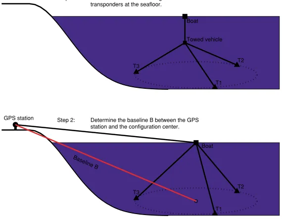
Step 1: Determine the internal configuration of the transponders at the seafloor.

Boat

Towed vehicle

T1 T2 T3

Step 2: Determine the baseline B between the GPS station and the configuration center.

Boat

T1 T2 T3

GPS station

Baselin e B

Fig. 1. Illustration of the SIO method. The upper plot has illustrated the determination of the internal configuration of the SIO method by towing a vehicle a few hundred meters above the seafloor, which consists of three transponders on the seafloor ideally distributed uniformly along a circle; the lower plot has shown the determination of the baseline marked in red by keeping the boat moving within a small area on the sea surface above the configuration center, and by using kinematic GPS and acoustic measurements.

and underwater acoustics (see e.g. Spiess, 1980, 1985a, b; Purcellet al., 1990; Fujimotoet al., 1995; Chadwellet al., 1998; Fujimotoet al., 1998; Spiesset al., 1998; Obanaet al., 2000; Asada and Yabuki, 2001; Yamadaet al., 2002; Chadwell, 2003). The technique consists of two basic com-ponents: (i) precise kinematic GPS; and (ii) precise under-water acoustics. Precise kinematic GPS serves three pur-poses in this seafloor geodetic positioning system: (i) to determine the position of the ship in real time; (ii) to de-termine the attitude of the ship for precise computation of the position of the transducer installed under the hull of the ship; and (iii) to connect the local seafloor geodetic network to the global reference frame. Underwater acoustics is fun-damental in establishing a precise local seafloor geodetic network, however.

Seafloor geodetic positioning has been conducted in two different ways: (i) single point (transponder) positioning; and (ii) positioning the center of a configuration defined by three or four transponders. The starting observation equation for these two methods may be symbolically given in its simplest form as follows:

ρi j= f(xoi,xj)+δρdi j+δρvi j +i j, (1)

where ρi j is the ranging between the ith transponder on

the seaﬂoor and the transducer under the ship, which can be calculated from the travel time and the sound velocity structure. f()is a nonlinear functional of ray tracing, xoi

is the unknown position of theith transponder. xj is the

position of the transducer, which can be directly calculated from kinematic GPS. δρdi j is the systematic error due to

the time delay in re-transmitting the received signal from the transponder back to the transducer,δρ_vi j the systematic

error due to the spatial and temporal variation in the sound velocity structure, in particular, in the area of upper 500 meters under the sea surface (Spiess, 1985a; Fujimoto et

al., 1995; Chadwellet al, 1998; Lurton, 2002). This error varies from one observation to another, depending on both separation in time and space. i j is the random ranging

error. With modern transponders,δρdi j would be at the level

of millimeters and could be negligible, correspondingly,i j

is reported to be at the level of one centimeter (Chadwellet al., 1998). The most damaging factor in seaﬂoor geodesy is due toδρ_vi j, which can reach some hundreds of ppm, or

equivalently, the error of sound velocity in a few parts in 104(Spiess, 1985a).

In the case of single point positioning, Yamada et al.

(2002) showed by simulations that the effect ofδρvi j on the

position of a transponder can reach 18 cm. In fact, this dam-aging effect was fully recognized in the very beginning of seafloor geodetic positioning. In order to eliminate the ef-fect of this most important error source, the group of the Scripps Institution of Oceanography (SIO) has followed the proposal by Peter Bender, installed three or four transpon-ders uniformly in a circle, kept the survey ship around the center of the configuration and determined the horizontal components of the position of the rigid polygon formed by transponders (see e.g. Spiess, 1985a; Chadwellet al., 1998; Spiesset al., 1998; Chadwell, 2003). We will refer to this positioning strategy as the SIO method in the rest of this pa-per. The SIO method is illustrated in Fig. 1 and consists of two basic steps: one to determine the internal configuration of the three (or four) transponders on the seafloor and the other to determine the baseline between the GPS station on land and the (non-physical) center of the polygon formed by the transponders. Due to the symmetry of the transpon-ders and simultaneity of measurement of the ranges,δρ_vi j

are identical if the sound velocity is assumed to vary with depth only. As a result, it is clear mathematically that the ef-fect ofδρ_vi j has cancelled out in the horizontal components

(3)

and by assuming the relative positions of the transponders do not change in time, the repeatability of horizontal com-ponents was reported to be about 4 cm (Chadwell et al., 1998; Spiesset al., 1998) and more recently to be less than 10 mm (Gagnon et al., 2005). However, changes in the sound velocity directly affect the vertical component.

The major purpose of this paper is twofold: (i) to de-velop a new strategy to position a single transponder at the centimeter level of accuracy; and (ii) to investigate the fea-sibility to establish a seafloor geodetic network for precise seafloor deformation measurement. The paper is organized as follows. In Section 2, we propose a new single point positioning method by differencing the ranging measure-ments between two consecutive ship positions. A theoret-ical comparison with the SIO and other methods will be briefly given. In Section 3, we investigate the feasibility of establishing a seafloor geodetic network by combining the new differencing technique with more ranging and pressure data from a vehicle towed a few hundreds meters above the seafloor. In Sections 4 and 5, we will discuss the experiment design and carry out simulations to investigate the accuracy improvement of the new seafloor positioning method and the accuracy improvement of a seafloor geodetic network for precise seafloor deformation measurement.

2. New

Approach

to

Positioning

a

Single

Transponder

The most fundamental advantage of the SIO method over the current single point seaﬂoor positioning is in that the SIO method is almost free of the effect of long and short pe-riod systematic errorδρvi j due to variations in sound

veloci-ties under the assumption thatδρ_vi j depends on water depth

only. High precision in horizontal components is achieved by installing three or more transponders on the seafloor and by strictly controlling the survey vessel within a small area around the center of the circle defined by these three or four transponders. In this section we develop a technique to position a single transponder. This technique eliminates the long period systematic effect as does the SIO method. Short-period effects remain, but in a later section we show they are reduced by requiring the vessel to follow a symmet-rical track around the transponder and then averaging these data or if the speed of the vessel is sufficiently fast such that the time between two measurements is much shorter than the period of these effects.

2.1 Mathematical model

We assume that the survey ship is at the positionsxi at

timetiandxj at timetj.xiandxjare given, since they can

be determined from kinematic GPS. We also assume that there is a single transponder on the seaﬂoor, whose position

xois to be determined from kinematic GPS and underwater

acoustic ranging measurementsρsioandρsjo.The surveying

strategy is illustrated on the left part of Fig. 2. As in (1), we have two observation equations:

ρsio= f(xo,xi)+δρdsi o+δρvsi o+i o, (2a)

ρsjo= f(xo,xj)+δρds j o +δρvs j o+j o, (2b)

where f(xo,xi) and f(xo,xj) are the ranges computed

from transponder and GPS positions, δρd_{si o} andδρd_{s j o} the

systematic errors associated with the travel time,δρ_v_{si o}and

δρvs j othe systematic errors associated with the sound speed,

i o andj o the combined random errors of the travel time

and sound speed.

The linearized version of (2) is given as follows:

ρsio− f(x

ﬁrst partial derivatives of f()with respect toxo and

com-puted withx0

o,xi andxj, respectively. dxois the unknown

coordinate correction vector to be estimated. bsio andbsjo

are the ﬁrst partial derivatives with respect toxiandxj,

re-spectively. xsi andxs j are respectively the random errors

of the survey vessel positionsxiandxj.

Applying the difference operator to two consecutive acoustic rangings by substracting (3b) from (3a), we have:

ρi j=(asio−asjo)dxo+ρdsi j o+ρvsi j o+i j o, (4a)

Now assume that the two vessel positionsxi andxj are

taken consecutively and are sufﬁciently close in space and time, then it is reasonable to believe that the two rays be-tween the transducer and the transponder go through the same sound velocity structure. As a consequence, we should expectδρ_v_{si o} ≈δρ_v_{s j o}.In other words, the third term

ρvsi j o on the right hand side of (4a) should be equal or

almost equal to zero. However, if the variation of sound ve-locity is of a short period, due to internal waves, for exam-ple, then the effect ofρv_{si j o}on the position of the transpon-der can still be signiﬁcant. Therefore our observation equa-tion retains an unknown bias term for each single difference observation. We will later show that the impact of this bias can be reduced by selecting a symmetrical ship track and averaging the data. On the other hand, since the ranging measurementsρsioandρsjoare taken on the same

transpon-der, the time delays in re-transmitting the signals back to the transducer should remain unchanged as well. Thus the second term ρd_{si j o} on the right hand side of (4a) can be

treated as zero.

Hence, given two consecutive and sufﬁciently close ves-sel positionsxi andxi₊1, the observation equation (4a) can

be simpliﬁed as follows:

ρi(i+1)=(asio−asi+1o)dxo+i(i+1)o, (5)

(4)

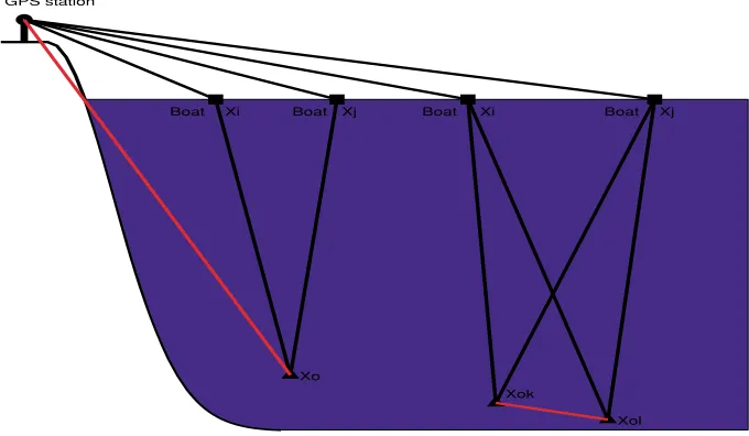
Xi

Xo Xj

Boat Boat Xi

Xok

Xol Xj Boat Boat GPS station

Fig. 2. Illustration of the new single- and double-difference methods. The left and right parts of the ﬁgure have illustrated the single- and double-difference processing strategies, respectively. In the single-difference mode, the major interest is in determining the baseline marked in red or simply the positionxoof the transponder on the seaﬂoor; in the double-difference mode, the interest is in precisely determining the baseline

between two transponders on the seaﬂoor, which is also marked in red betweenxok andxol.

that the time for the ship to move from one position to next is negligibly short compared with the short period effect. By collecting all the observation equations of this type together, we have the system of linear observation equations:

y=Adxo+ y. (6)

It is obvious from (5) or (6) that the estimate ofdxo from

the differenced ranging measurements is free of systematic errors of long wave nature. Although systematic errors of short wavelength may still retain due to the current practice of a slow ship speed, they will be negligible with advance of technology such that a ship can move sufﬁciently fast. As a result, we will not include the bias term in our equation.

2.2 Stochastic model

As in the single point positioning or the SIO method, the seaﬂoor geodetic positioning system (6) is inﬂuenced by all the random error sources. Since (6) is based on dif-ferenced ranging measurements, the computed observations cannot be treated as independent. The variance-covariance matrices of the transducer positions at the timesti andtj

are denoted by Σsi and Σs j, respectively. Here the

er-rors of the transducer position can be derived from those in kinematic GPS positioning, attitude determination and op-tical/laser surveys. The latter two techniques are needed to derive the position of transducer from the kinematic GPS position. Since optical/laser survey, for example, by using a total station, can be very precise at the millimeter level, its effect on the variance-covariance matrix could be negligi-ble. According to Cohen (1996), the angular accuracy from attitude determination can be estimated by

σθ= 0.5 cm

L (in cm). (7)

Given the antenna conﬁguration of Chadwell (2003), the accuracies of roll and pitch would be about 1.17 minutes and 0.47 minutes, respectively. If one of the antennas is

mounted within 10 meters from the transducer, then the correction error due to those of attitude determination will be a few millimeters, which is more than one magnitude smaller than the error of kinematic GPS positioning. Thus it is safe to simply replace the variance-covariance matrix of the transducer position with that from kinematic GPS positioning.

Further assume that the sound ranging measurements are stochastically independent and have an accuracy ofσ_ρ. Then by applying the error propagation law to (4e), we can compute the variance of the differenced measurement:

σ2 ρi j =2σ

2

ρ+bsioΣsib

T

sio+bsjoΣs jb

T

sjo, (8)

where the superscriptT stands for the transpose of a matrix or vector.

In the similar manner, for any two consecutive differ-enced ranging measurementsρi(i+1)andρ(i+1)(i+2), we

can compute the covariance between them as follows:

cov(ρi₍i₊1), ρ(i₊1)(i₊2)) = −σ2

ρ−bs₍_i+1)oΣs(i+1)bTs(i+1)o. (9)

Because we have assumed that GPS positioning errors and sound speed errors are uncorrelated with time, ρi j and ρklare uncorrelated ifk−j>1.Under these assumptions

the full variance-covariance matrix of the (differenced) ob-servation vectorycan be completely obtained from (8) and (9), which is denoted by Σyand is a positive deﬁnite matrix

with a bandwidth of one only.

2.3 Least squares estimate of dxo and ﬁrst

compar-isons with other methods

Applying the least squares method to (6), we can readily obtain the estimate of the position correction dxo of the

transponder on the seaﬂoor as follows:

dxo=(AT Σ−1y A)−1A T _Σ−1

(5)

from which we can compute the ﬁnal transponder position

ˆ

xo =x0o+dxo, (10b)

and its variance-covariance matrix Σx_ˆo

Σxˆo =(A

T _Σ₋1

y A)−1. (10c)

Comparing (10) with the single transponder positioning in the literature (see e.g. Yamadaet al., 2002), we see that the new approach (10) is free of long term systematic ef-fects. Short term biases may retain, unless the ship moves sufficiently fast. If the number of differenced measurements has been accumulated such that sufficient strength of geom-etryAis obtained and that short term effects can be aver-aged to zero, then one centimeter accuracy of position can be obtained for the transponder on the seafloor, which will be confirmed in Section 5 by simulations.

Comparing (10) with the SIO method, we see that both methods are not affected in the horizontal components of the transponder position by systematic errors due to het-erogeneity in the sound velocity structure. Unlike the SIO method, the new positioning method can also produce the precise vertical component. Neither approach is biased by time delay in the re-transmission of signal from the transponder. The new approach differences this away by assuming that the magnitude of the delay does not change appreciably as the aspect and azimuth angle at the trans-ducer changes from the first to the second range used to form the difference. The SIO approach keeps the same as-pect and azimuth angle between the shipboard and seafloor transponders so this bias is constant and is cancelled out in determining the polygon center of the array. The new method positions a single transponder by developing a new data processing strategy and by requiring the survey ves-sel to either move freely if the speed of the vesves-sel moves sufficiently fast or to maneuver along a symmetrical track around the transponder in the current situation of slow ship speed. The SIO method uses 3 or 4 transponders and re-quires the ship hold station at the center of the transpon-der array. The new method measures the displacement of a single transponder while the SIO method measures the displacement of the patch of seafloor defined by the poly-gon formed by the transponders. Thus the new method can provide a finer spatial resolution of the deformation field. This can be of particular importance in regions with signifi-cant local strain, where the SIO method must collect data to re-determine the internal configuration of the transponders. The SIO method is free of long and short period errors in sound speed, while the new single difference method re-quires a to-be-determined track to be driven to accumulate enough changes in geometry such that the average effect of biases is near zero, unless the ship moves sufficiently fast such that the time between two ship positions is sufficiently short to neglect the short period effect.

3. Seaﬂoor Geodetic Network

Given a seaﬂoor geodetic network deﬁned by a number of transponders, we could use the single positioning method described in the previous section to precisely determine the

positions of all the transponders. With the rapid advance-ment of technology, precise measureadvance-ments other than ar-rival times between the transducer on the survey vessel and the transponders on the seafloor are expected. For instance, in the case of the SIO method, a lot more of ranging mea-surements have been collected by towing a measuring unit at about a few hundreds meters above the seafloor. In ad-dition, height differences between the hydrophone mounted on the towed unit and the transponders can also be com-puted (see, e.g., Spiess, 1985b; Chadwell et al., 1998; Spiess et al., 1998; Sweeney et al., 2005). Fujimoto et al. (1995, 1998) also did a lot of experiments on measur-ing the distance between two transponders on the seafloor and reported that if poor data are removed, the ranging error would reach one or two centimeters.

In this section, we will combine these measurements with usual ranging measurements between the survey vessel and transponders on the seafloor described and used in the previ-ous section into a seafloor geodetic network, and investigate how these extra measurements will improve the accuracy of seafloor geodetic positioning. Given a seafloor geode-tic network withmtransponders properly distributed on the seafloor, assuming that in addition to the ranging measure-ments between the transducer mounted on the survey ves-sel and the transponders on the seafloor, we also collect the height differences and ranging measurements through the towed hydrophone at about a few hundreds meters above the seafloor.

3.1 Measurements collected by towed hydrophones

Since the observation equations for the measurements be-tween the vessel and the transponders have been given in the previous section, we will focus on the height differ-ences and ranging measurements collected by the towed hy-drophone here. Assume that the towed hyhy-drophone at the timeticollect data from a subset ofmi transponders on the

seaﬂoor, which is denoted by(1,2, . . . ,mi). Then for any

height differencehi jbetween the towed hydrophone and the

jth transponder, we have the observation equation:

hi oj =H(xi,xoj)+hi j, j ∈(1,2, . . . ,mi) (11)

where H(·)is the functional deﬁned by ray tracing, xi is

the position of the towed hydrophone at the timeti, which is

unknown and to be determined.xoj is the unknown position

of the jth transponder or station of the seaﬂoor geodetic network. hi j is the observation error ofhi j. According to

Spiess (1985b) and Spiesset al.(1998), the accuracy ofhi oj

would be about 5 centimeters.

Linearizing (11) results in the equations:

hi oj−H(x

Similarly to (3a), and bearing in mind that unlikexi of

(3a),x0

i is not random but unknown to be determined, the

(6)

the jth transponder can be linearized as follows:

respect to xoj andxi, respectively. Since the systematic

errors due to the heterogeneity of sound velocity structure at deep sea and the time delay are rather small, if they are neglected from (13), then we have

ρi oj − f(x

However, as a remedy, although the noise of ranging mea-surements could reach one cm or be better, the accuracy of ranging measurements and height differences has been set to 10 and 5 cm, respectively (see, e.g. Spiess, 1985b; Spiess

et al., 1998).

Collecting all the linearized observation equations (12) and (14) through the whole seaﬂoor geodetic network to-gether, we have the ﬁnal system of linearized observation equations:

yt =AtdX+ t, (15)

whereyt stands for all the values on the left hand sides of

(12) and (14) taken from the towed unit,Atis the coefﬁcient

matrix, t is the error vector ofyt, and

dX= {dxT_o₁,dxT_o₂, ...dxT_o_m,dxT₁,dx₂T, . . . ,dx_qT}T.

Hereqis the total number of time epoches of data taken by the towed unit.

In the single point positioning mode, all the positions of transponders can be independently determined, for which we only need to solve a(3×3)normal matrix. This is not true any more in the case of (15). Putting all the observation equations (6) and (15) together, we are ready to solve the seaﬂoor geodetic network. In the network mode, we have to solve a {3(m+q)×3(m +q)} normal matrix, since all the unknownsdxoi {i ∈ (1,2, . . . ,m)} anddxj {j ∈

(1,2, . . . ,q)}are intermingled together through (12) and (14).

3.2 More difference operators for use in the network

mode

Alternatively, instead of using the difference (4a) be-tween two ranging measurements taken at different time epoches, in the network mode, we can also difference two ranging measurements between different transponders taken at the same time epoch. Assume that the vessel-mounted hydrophone at the timeti collect data from a

sub-set ofmitransponders on the seaﬂoor, which is denoted by (1,2, . . . ,msi). In a similar manner to (3a), we have

the right part of Fig. 2).

Applying the difference operator to (16) by taking (16b) from (16a), we have the new difference ranging measure-ment

As in the case of single point positioning, (17d) would be equal to zero, if the variation in sound velocity is assumed to be depth-dependent within the circle with radius of a few kilometers. Since the difference is taken at the same time epoch, variations with a short period of few minutes to hours such as effect of potential internal waves will also be eliminated by the difference operator (17d). Nevertheless, if the sound speed structure is horizontally stratiﬁed, the spatial effect will retain and (17d) will reﬂect this effect. However, since∇ρi

dklis involved with two transponders, the

effect of time delays cannot be eliminated, unless they are negligible.

In a similar manner to (17a), we can write another differ-ence measurement for the time epochtj as follows:

∇ρj

zontally stratiﬁed structure of sound speed. Now applying the difference operator further to (17a) and (18), we have the double-difference measurement

The time delays has been completely eliminated in the double-difference measurement and thus have no effect on positioning.

If the two consecutive positions of the ship are sufﬁ-ciently close, ∇ρi

vkl and∇ρ

j

vkl cancel out each other, and ∇ρi j

vkl is equal to zero. Thus (19) can be further simpliﬁed

as follows:

∇ρi j

kl =(ai ok−aj ok)dxok−(aj ok−aj ol)dxol+∇

i j kl. (20)

(7)

advantage of applying double difference should be obvious. Similarly, one can also apply these difference operators to the measurements collected from the towed hydrophone(s), which is omitted here.

By combining (20) with the equations of type (5) and those from the towed hydrophone(s), and by using the method of previous section to derive thea priori variance-covariance matrix, we can apply the least squares method to solve for all the positions of the transponders on the seaﬂoor in the network mode.

4. Experiment Design

We will design a number of experiments in this section to demonstrate the attainable accuracy by the new differ-ence methods for a single point seafloor positioning and network mode, and potential accuracy improvement by in-cluding more data in the network mode. Since geometric topologies of ray paths in the oceanic environment are sim-ilar or only slightly different between the depth-dependent and constant speed structures (Lurton, 2002), we will sim-ply use the latter for establishing observation equations in our simulations for simplicity and focus on the effect of sys-tematic and random errors on seafloor geodetic positioning. This simplification may be sufficient for our accuracy sim-ulation, since the sound velocity variability due to internal waves has negligible effect on the take-off angle (Flatté and Vera, 2002), and as a result, also negligible effect on the co-efficients of the observation equations in the previous sec-tions. In practical applications, we should write observation equations based on Snell’s law of refraction and compute the position of the transponder on the seafloor or adjust the seafloor geodetic network by using a modelled or measured sound velocity structure, however.

The experiment design for seafloor geodetic ing consists mainly of four parts: (i) design of position-ing modes, namely, sposition-ingle point positionposition-ing or network; (ii) selection of difference operators; (iii) models for sys-tematic errors in ranging measurements; and (iv) models for random errors of GPS/acoustic measurements. We de-sign two single point positioning experiments with differ-ent sample spacings along the trajectory of the survey ves-sel, respectively. We also design two relative seafloor po-sitioning experiments—the simplest geodetic networks on the seafloor, whose stations (transponders) are separated by 1 km, respectively. Since measurements in network mode are collected from, at least, a few hundreds meters above the seafloor, the shape of network triangles can be best cho-sen practically without loss of generality. Keeping in mind possible direct applications of the simulation results in this paper to monitoring the source area of the Nankai earth-quakes, we decide to choose the water depth of 3000 m. In order to avoid or minimize the effect of multipath, the vessel is allowed to move within a square area with length roughly equal to the depth of water.

In order to simulate systematic errorsδρ_v, we consider in Eq. (21) the four types of effects: (i) a constant term; (ii) internal wave with a short period; (iii) diurnal and/or (semi-)diurnal tides; and (iv) factors of regional effect by using a Gaussian correlation function. More speciﬁcally,

we simulate the systematic errors in centimeters as follows:

δρv =c1+c2sin

Since the effect at the mesoscale of hundreds and/or thou-sands km should produce the same effect over a small area, we may attribute such an effect to the ﬁrst constantc1.

Ac-cording to Flatt´eet al.(1979) and Colosiet al.(1994), the effect of internal wave on sound velocity could be ﬁve parts in 104_{at the surface and one part in 10}4_{at the depth of 1}

km. Although internal wave has been always treated as a random phenomenon in ocean acoustics (see e.g. Flattéet al., 1979; Colosiet al., 1994; Desaubies, 1990; Flatté and Vera, 2002), we have to treat it as a source of systematic errors and have to remove or eliminate its effect on seafloor positioning for precise seafloor deformation measurement. A diurnal error with an amplitude of about 20 ∼ 30 cm can also be seen clearly in Spiess et al. (1998). Taking all these into account, we have chosen the four constants

c1 =10,c2 =12 as in Yamadaet al.(2002),c3 =30 and c4=2. The time units in the second and third terms on the

right hand side are in minutes and hours, respectively, with

Tw =20. x−xis the length between the pointsxand

x. Three ranging errors of 1, 5 and 7 cm will be used in our simulations, and that of height differences is assumed to be 5 cm. The accuracy of GPS kinematic positioning is assumed to be 10 cm. We should note that if the ship is far away from land such that GPS integer ambiguity un-knowns cannot be correctly ﬁxed, then kinematic GPS will not be able to provide the position accuracy of 10 cm. In this case, one may have to either consider using some inter-mediate means (one more ship, for example) to bridge land GPS stations and the surveying vessel or simply treat the seaﬂoor geodetic network as a free network. Since we do not have thea prioriinformation on the correlations among the three components, we simply assume x is normally

distributed with mean zero and variance-covariance matrix

σ2

5.1.1 Positioning by using the SIO method As the

(8)

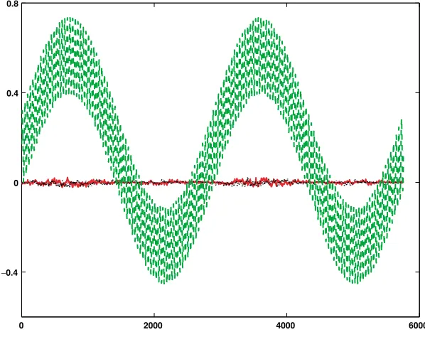
0 2000 4000 6000 −0.4

0 0.4 0.8

Fig. 3. The effects of systematic errors on the SIO method (unit: meters). The horizontal axis marks the sampling epochs. The effects of systematic errors on the SIO method are shown in the red solid and black dotted lines (the horizontal components) and the green dashed line (the vertical component).

the simulated systematic errors on these two components is close to zero. However, the effect of the systematic errors on the vertical component (the green line in Fig. 3) remains uncancelled and is signiﬁcantly large, varying from−0.452 to 0.735 m with an average effect of 0.141 m.

We have to note that almost zero effect of systematic er-rors on the horizontal components reported above should not be confused with or interpreted as the final possible (extremely high) accuracy in the horizontal components by the SIO method, for two reasons: (i) random measurement errors and the effect of spatial variations in sound speed are not included in the above confirmation of the ability of the SIO method to remove the systematic effect of depth-dependent effect; and (ii) in order to derive the final posi-tioning accuracy, we have to consider the effect of the un-certainty in the internal configuration of the three transpon-ders uniformly distributed along a circle on the seafloor. In fact, the errors of the configuration center can be mathemat-ically written as follows:

i c=

i gps−

i

ρ−biρ+ xt, (22)

for each epoch of measurement, where the superscript stands for theith epoch, icis the error vector of the derived

conﬁguration center, igpsis due to the errors of kinematic

GPS, i_ρ is due to the random errors of ranges between the transponders and the transducer, bi_ρ is the systematic errors of the derived conﬁguration center due to (21), and xt is due to the errors of the internal conﬁguration of the

transponders. What we have shown in Fig. 3 are actually the bias term of bi

ρ with the changes of epochs. Almost

zero average effect of the systematic errors on the horizon-tal components can be obviously observed. Since the ﬁrst two terms on the right hand side of (22) are random and are dependent on the time epochs, their contribution to the

errors of the final averaged configuration center could be negligible if the number of epochs is sufficiently large. The effect of the errors in the internal configuration certainly does not change with epochs. If the relative positions of the transponders do not change throughout the experiment, then the biases cancel out. Using real data, Gagnonet al.(2005) have shown that the repeatability of the SIO method can be less than 10 mm. If the relative positions of the transpon-ders are likely to change, then they can be re-measured with a resolution of 2 cm using a deeply towed vehicle (Sweeney

et al., 2005). However, if there exist spatial variations in the sound velocity structure, the (horizontal) accuracy of the SIO method would deteriorate, the extent of which depends on the relative magnitude of the spatial variations.

5.1.2 Positioning by the difference method We will

now design a number of experiments to study the effective-ness of the difference method for precise seafloor position-ing. More specifically, we will investigate the effects of different factors on the single seafloor positioning by the difference method. These factors include: (i) differences in the accuracy of observations; (ii) short period of internal waves; (iii) sampling spacings; and (iv) different surveying strategies, which are shown in Fig. 4.

Given the vessel speed of 1 m/s and the sampling period of about 1.667 minutes for the circular surveying trajectory, we plotted in Fig. 5 the corresponding original systematic errors inρsio and those remaining in the differenced

obser-vationsρi j, with and without the effect of internal waves

of short period. In the case of no internal waves, namely,

c2 in (21) is equal to zero, then the remaining systematic

(9)

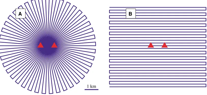
B A

1 km

Fig. 4. The two surveying strategies (trajectories) for testing the performance of the difference method: the solid lines—the surveying trajectories; the red triangles—the transponders on the seaﬂoor.

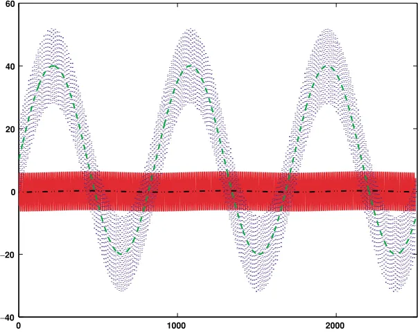
0 1000 2000

−40 −20 0 20 40 60

Fig. 5. The systematic errors of the original and differenced acoustic ranging measurements, with and without the effects of internal waves of short period. The horizontal axis marks the sampling epochs. The vertical axis is marked in centimeters. The original systematic errors are shown in the blue dotted and green dashed lines, with and without the effect of internal waves, respectively. The remaining systematic errors in the differenced acoustic ranging measurements are in the red solid and black dash-dotted lines with and without the effect of internal waves, respectively.

red line in Fig. 5 that a signiﬁcant part of systematic errors in the original acoustic ranging measurements still remains in the differenced measurements, varying from −6.22 to 6.22 cm with an average of 0.1 mm, basically due to the effect of internal waves of short period. Listed in Table 1 are the accuracy results of positioning from the circular (A) trajectory (compare Fig. 4) by using the difference method, with different accuracy of 1, 5 and 7 cm for acoustic rang-ing measurements ρsio, and with and without the effect of

internal waves of short period taken into account.

We can see from Table 1 that the difference method can result in subcentimeter level of accuracy in the horizontal

(10)

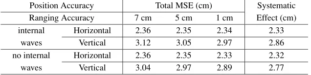
sur-Table 1. The accuracy of the seaﬂoor positioning from the circular surveying trajectory by using the difference method, with different acoustic ranging accuracy of 1, 5 and 7 cm, and with and without the effect of internal waves of short period. HorizontalandVerticalin the table stand for the horizontal and vertical components of the seaﬂoor transponder position, respectively.

Position Accuracy Total MSE (cm) Systematic

Ranging Accuracy 7 cm 5 cm 1 cm Effect (cm)

internal Horizontal 0.78 0.66 0.51 0.07

waves Vertical 1.98 1.69 1.33 0.49

no internal Horizontal 0.78 0.65 0.50 0.04

waves Vertical 1.92 1.62 1.24 0.03

Table 2. The accuracy of the seaﬂoor positioning from the rectangular surveying trajectory by using the difference method, with different acoustic ranging accuracy of 1, 5 and 7 cm, and with and without the effect of internal waves of short period.HorizontalandVerticalin the table stand for the horizontal and vertical components of the seaﬂoor transponder position, respectively.

internal Horizontal 2.36 2.35 2.34 2.33

waves Vertical 3.12 3.05 2.97 2.86

no internal Horizontal 2.36 2.35 2.33 2.32

waves Vertical 3.04 2.97 2.89 2.77

veying strategy can help greatly reduce or cancel out the effect of the remaining systematic errors on seafloor posi-tioning. This is very likely due to the fact that the remaining systematic errors due to the internal waves of short period after difference of measurements behave periodically and can thus be significantly reduced or cancelled out through a symmetrical design of surveying strategy, which looks more or less like the SIO method in cancelling out the effect of systematic errors through a uniform design of transponders and by confining the surveying vessel around the center of the configuration. However, unlike the SIO method, the dif-ference method can also produce the vertical component of a transponder at the accuracy of one or two centimeters. We can also conclude from this table that the accuracy of the horizontal and vertical components is mainly affected by the accuracy of kinematic GPS, since changing the accu-racy of acoustic rangings only slightly affect the positioning accuracy.

In the case of the rectangular (B) surveying strategy (compare the right plot of Fig. 4 and Table 2), the effects of the remaining systematic errors are still at the level of 2 to 3 cm such that they basically dominate the mean squared errors of positioning, although the final accuracy of posi-tioning is about 2.35 cm in the horizontal components and around 3 cm in the vertical component. These experiments have shown that (i) both surveying strategies can produce centimeters level of accuracy in seafloor positioning; (ii) the rectangular surveying strategy is less effective in re-ducing or removing the effects of systematic errors on pre-cise seafloor positioning than the circular surveying strat-egy. This might be explained as follows: the circular sur-veying route is horizontally symmetrical with respect to the transponder at every 6 km, while the rectangular route is only so after finishing a complete surveying route. In other words, the circular surveying strategy is some tens times

more effective in terms of symmetry than the rectangular one. As a result, the circular surveying strategy is more ef-fective in reducing the effect of residual systematic errors. We may also note that if acoustic signals are much stronger with the advance of technology in the future and are less affected by the noise of engine of the surveying ship, then the ship could move faster. With the decrease of time mov-ing from one point to next, the residual systematic errors should decrease as well; and (iii) a well-designed surveying strategy would be very helpful in improving the accuracy of seaﬂoor positioning.

(11)

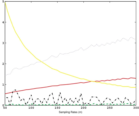
50 100 150 200 250 300 0

1 2 3 4 5

Sampling Rates (m)

Fig. 6. The effect of sample spacings on seaﬂoor positioning by the difference method, with the effects of internal waves of short period: the horizontal axis—the sample spacings in meters; the red solid line—the accuracy or root mean squared error (MSE) of the horizontal components; the blue dotted line—the accuracy or root MSE of the vertical component; the green dashed line—the systematic effect on the horizontal components due to the systematic errors; the black dash-dotted line—the systematic effect on the vertical component due to the systematic errors; the yellow solid line—the numbers of sample points corresponding to the sample spacings (unit: 1000 points). Except for the yellow line, the units in the vertical axis are all in centimeters for the other four lines.

both horizontal and vertical components to the level of 1 cm.

5.2 Relative seaﬂoor positioning

Relative seafloor positioning is to determine the relative position of two transponders on the seafloor by using the acoustic ranging measurements collected by the boat hy-drophone. It may be thought of as the simplest example of a seafloor geodetic network without use of the measure-ments collected by towed hydrophones. If there exist in-ternal waves of short period from minutes to tens of min-utes, it is theoretically expected in Section 2.1 and has been shown numerically in Section 5.1.2 (compare Fig. 5) that a significant part of systematic errors of short period nature (internal waves, for example) can still remain in the single difference measurements, and can significantly affect accu-racy on seafloor positioning, the extent of which is related to surveying strategies, however. We have also learnt from Section 3.2 that if two consecutive sample points are suf-ficiently close, spatial and temporal effects of systematic errors can all be removed. Thus we will use the double dif-ference method to determine the relative position between two transponders on the seafloor.

Without loss of generality, we will ﬁx one of two transponders and focus on the determination of the relative vector, which is denoted byx. Then the observation equa-tions of type (20) can be written as

∇ρ(i+1)i₍

x)=(ai o2−a(i+1)o2)δx+(i+1)i, (23)

where

(i+1)i =(ai o1−ai o2)xi −(a(i+1)o1−a(i+1)o2)xi+1

−i o1+i o2+(i+1)o1−(i+1)o2.

In order to investigate the accuracy of seafloor position-ing by the double difference method, we design the circular and rectangular surveying trajectories to measure the rela-tive position between two transponders (Fig. 7). We assume the radius of depth plus half of the vectorxfor the circu-lar trajectory. In the case of rectangucircu-lar trajectory, the area is equal to the diameter of the circular trajectory multiplied by two depths. In our experiments, we assume that the two transponders are separated by 1 km. As in Section 5.1.2, we use the sampling rate of about 1.667 minutes for the circular surveying trajectory. Since the effect of systematic errors has been almost completely eliminated by the dou-ble difference operator, we will focus on the random effect on seafloor positioning. The kinematic GPS will still be as-sumed to provide the position of the surveying boat at the accuracy of 10 cm, while acoustic ranging measurements between the boat hydrophone and the transponders on the seafloor are of the accuracy of 1, 5 and 7 cm, respectively.

(12)

B

1 km A

Fig. 7. The two surveying strategies (trajectories) for testing the performance of the double difference method: the solid lines—the surveying trajectories; the red triangles—the transponders on the seaﬂoor.

Table 3. The accuracy of the relative seaﬂoor positioning from the circular (A) and rectangular (B) surveying trajectories by using the double difference method, with different acoustic ranging accuracy of 1, 5 and 7 cm.HorizontalandVerticalin the table stand for the horizontal and vertical components of the seaﬂoor transponder position, respectively.

circular Horizontal 0.79 0.57 0.15

trajectory Vertical 1.79 1.29 0.36

rectangular Horizontal 0.60 0.43 0.11 Eliminated

trajectory Vertical 1.68 1.21 0.33

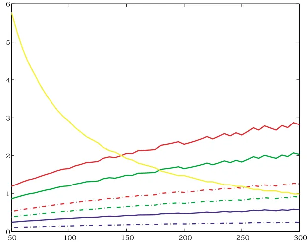
shortened in time to achieve sub-centimeters level of accu-racy for relative seaﬂoor positioning. We have also shown in Fig. 8 the variations of accuracy for the circular trajec-tory at the accuracy of 1, 5 and 7 cm for acoustic ranging measurements. It can be seen that the accuracy of relative seaﬂoor positioning can be as good as sub-centimeters in the horizontal components for all the three cases, and is be-tween 1 and 3 cm in the vertical component in the cases of 5 and 7 cm, and reaches again sub-centimeters in the case of 1 cm. Even for the former two cases, if more data are collected on sea, sub-centimeters accuracy for the verti-cal component should also be expected, since this would be equivalent to increasing the accuracy for acoustic ranging measurements.

6. Concluding Remarks

Seafloor geodesy has been developed for measuring seafloor crustal deformation by Spiess (1980, 1985a, b), based on the idea of Peter Bender by installing three or four transponders uniformly along a circle on the seafloor and by keeping the surveying vessel as close to the center of the circle as possible. Such a surveying strategy has been shown to be effective in precisely determining the horizon-tal components of the configuration center, since system-atic errors have been cancelled out. However, the effect of systematic errors on the vertical component remains un-changed. The repeatability for the horizontal components

obtained by the group of researchers at the Scripps Institu-tion of Oceanography was recently reported to be less than 10 mm (Gagnonet al., 2005). In regions of local deforma-tion, the SIO method requires the internal geometry of the transponders to be re-determined by using a deeply-towed vehicle.

(13)

Fig. 8. The effects of sample spacings and acoustic ranging errors on the accuracy of relative seaﬂoor positioning. The horizontal axis shows the sample spacings in meters along the trajectory. The units in the vertical axis, except for the yellow line, are in centimeters. The two red, green and blue lines correspond to the accuracy of 7 cm, 5 and 1 cm for acoustic ranging measurements, respectively. The dash-dotted and solid lines show the accuracy in the horizontal and vertical components, respectively. The yellow line marks the numbers of sample points for each sample spacing (units: 1000 points).

must note that if the symmetry of surveying scheme is not kept, the remaining part of systematic errors (of short pe-riod) may prevent us from determining the transponders at the centimeters accuracy.

We have also conducted the experiments to determine the relative position between two transponders on the seafloor by using the double difference method. Unlike the single difference method, the double difference method is also able to remove the effect of systematic errors of short pe-riod, internal waves with period of minutes to tens of min-utes, for example, on relative seafloor positioning, if the two consecutive sampled points are sufficiently close. As a result, the double difference method is basically affected only by random errors. The simulations have shown that the three-dimensional, relative position between two transpon-ders separated by 1 km on the seafloor can be measured at the sub-centimeters level of accuracy, given the accuracy of 10 cm for kinematic GPS and the accuracy of 1, 5 and 7 cm for acoustic ranging measurements. Although the at-tained accuracy is derived with the symmetry of surveying scheme, this is not essentially needed by the double differ-ence method. Thus the efficiency of field work on sea can be significantly improved if the signals of transponders are sufficiently strong. If many transponders are installed on the seafloor and, if measurements collected by towed hy-drophones are included and processed together with acous-tic ranging measurements collected by the on-board hy-drophone in double difference mode, we are able to estab-lish a seafloor geodetic network for precise seafloor crustal deformation measurement.

Acknowledgments. The authors thank Dr. M. Fujita for the con-structive comments. They are also indebted to an anonymous

re-viewer for constructive comments, for polishing the English of the text and for bringing the two recently published articles to their attention. The work of the ﬁrst author is supported by a Grant-in-Aid for Scientiﬁc Research C(2)16540386.

References

Anderson, G., S. Constable, H. Staudigel, and F. Wyatt, A seaﬂoor long-baseline tiltmeter,J. Geophys. Res.,B102, 20269–20285, 1997. Ando, M., Source mechanisms and tectonic signiﬁcance of historical

earth-quakes along the Nankai Trough, Japan,Tectonophys.,27, 119–140, 1975.

Asada, A. and T. Yabuki, Centimeter-level positioning on the seaﬂoor,

Proc. Japan Acad. Ser. B,77, 7–12, 2001.

Chadwell, D., Shipboard towers for Global Positioning System antennas,

Ocean Eng.,30, 1467–1487, 2003.

Chadwell, D., F. Spiess, J. Hildebrand, L. Young, G. Purcell, Jr., and H. Dragert, Deep-sea geodesy: Monitoring the ocean ﬂoor,GPS World,9, 44–55, 1998.

Cohen, C. E., Attitude determination, inGlobal Positioning System: The-ory and Applications, Vol. II, edited by B. W. Parkinson, J. J. Spilker, Jr., P. Axelrad and P. Enge, pp. 519–538, Amer. Inst. Aeronautics & Astronautics, Washington, 1996.

Colosi, J. A., S. M. Flatt´e, and C. Bracher, Internal-wave effects on 1000-km oceanic acoustic pulse propagation: Simulation and comparison with experiment,J. Acoust. Soc. Am.,96, 452–468, 1994.

Desaubies, Y., Ocean acoustic tomography, inOceanographic and Geo-physical Tomography, edited by Y. Desaubies, A. Tarantola, and J. Zinn-Justin, pp. 159–202, Elsevier, Amsterdam, 1990.

Flatt´e, S. M. and M. D. Vera, Internal-wave time evolution effect on ocean acoustic rays,J. Acoust. Soc. Am.,112, 1359–1365, 2002.

Flatt´e, S. M., R. Dashen, W. H. Munk, K. M. Watson, and F. Zachariasen,

Sound Transmission trough a Fluctuating Ocean, Cambridge University Press, Cambridge, 1979.

Frank, F. C., Deduction of earth strains from survey data,Bull. Seismol. Soc. Am.,56, 35–42, 1966.

Fujimoto, H., T. Kanazawa, and H. Murakami, Experiment on precise seaﬂoor acoustic ranging—A promising result of observation,J. Seis-mol. Soc. Japan,48, 289–292, 1995 (in Japanese).

(14)

1998.

Gagnon, K., C. D. Chadwell, and E. Norabuena, Measuring the onset of locking in the Peru-Chile trench with GPS and acoustic measurements,

Nature,434, 205–208, 2005.

Gordon, R. G. and S. Stein, Global tectonics and space geodesy,Science, 256, 333–342, 1992.

Lambeck, K.,Geophysical Geodesy: The Slow Deformations of the Earth, Clarendon Press, Oxford, 1988.

Lurton, X.,An Introduction to Underwater Acoustics, Springer, London, 2002.

Obana, K., H. Katao, and M. Ando, Seaﬂoor positioning system with GPS-acoustic link for crustal dynamics observation—a preliminary result from experiments in the sea,Earth Planets Space,52, 415–423, 2000. Prescott, W. H., The determination of displacement ﬁelds from geodetic

data along a strike slip fault,J. Geophys. Res.,B86, 6067–6072, 1981. Purcell, G. H., L. E. Young, S. K. Wolf, T. K. Meehan, C. B. Duncan, S. S.

Fisher, F. N. Spiess, G. Austin, D. E. Boegeman, C. D. Lowenstein, C. Rocken, and T. M. Kelecy, Accurate GPS measurement of the location and orientation of a ﬂoating platform,Mar. Geod.,14, 255–264, 1990. Shimamura, H. and T. Kanazawa, Ocean bottom tiltmeter with acoustic

data-retrieval system implanted by a submersible,Mar. Geophys. Res., 9, 237–254, 1988.

Spiess, F. N., Acoustic techniques for marine geodesy,Mar. Geod.,4, 13– 27, 1980.

Spiess, F. N., Suboceanic geodetic measurements,IEEE Trans. Geosc. Remote Sens.,GE-23, 502–510, 1985a.

Spiess, F. N., Analysis of a possible sea ﬂoor strain measurement system,

Mar. Geod.,9, 385–398, 1985b.

Spiess, F. N., D. Chadwell, J. A. Hildebrand, L. E. Young, G. H. Purcell, Jr., and H. Dragert, Precise GPS/acoustic positioning of seaﬂoor refer-ence points for tectonic studies,Phys. Earth Planet. Int.,108, 101–112, 1998.

Sweeney, A. D., C. D. Chadwell, J. A. Hildebrand, and F. N. Spiess, Centimeter-level positioning of seaﬂoor acoustic transponders from a deeply towed interrogator,Mar. Geod.,28, 39–70, 2005.

Webb, S. C., Broadband seismology and noise under the ocean,Rev. Geo-phys.,36, 105–142, 1998.

Webb, S. C., T. K. Deaton, and J. C. Lemire, A broadband ocean-bottom seismometer system based on 1-Hz natural period geophone,Bull. Seis-mol. Soc. Am.,91, 304–312, 2001.

Yamada, T., M. Ando, K. Tadokoro, K. Sato, T. Okuda, and K. Oike, Error evaluation in acoustic positioning of a single transponder for seaﬂoor crustal deformation measurements,Earth Planets Space,54, 871–881, 2002.