On the equatorial virtual pole distribution

(1)

On the equatorial virtual pole distribution

Ji-Cheng Shao1_{, Mike Fuller}2_{, and Yozo Hamano}1

1_{Department of Earth and Planetary Science, University of Tokyo, Tokyo 113-0033, Japan} 2_{HIGP/SOEST, University of Hawaii at Manoa, HI 96822, USA}

(Received September 5, 2003; Revised April 27, 2004; Accepted May 1, 2004)

In this paper, we show that the Virtual Geomagnetic Pole (VGP) distribution used in paleomagnetic studies is only one of the 2D spherical projections of a 3D paleomagnetic directional data set. Therefore, in principle, the VGP distribution does not by itself completely represent the paleomagnetic directional data set. We suggest that it is necessary to include in the analyses another 2D spherical projection of a 3D paleomagnetic directional data set— the Equatorial Virtual Pole (EVP) distribution. The EVP is defined as the point 90◦from the VGP along the great circle through the VGP and the site. The VGP and EVP distributions represent different aspects of the directional data sets and information not carried in the VGP distribution is carried by the EVP distribution. Ideal VGP and EVP distributions depict different aspects of the characteristics of the geomagnetic field as such that, while the VGPs tend to distribute symmetrically around the regions where the field is perpendicular to the earth’s surface, the EVPs concentrate about the nodal or null flux lines.

Key words:Virtual Geomagnetic Pole, paleomagnetism, point distribution, directional data.

1. Introduction

The paleomagnetic measurements are usually given as a set of the free unit vectors distributed on the earth’s surface representing the directions of the ancient geomagnetic field. The directional data set (DDS) of this kind may be equiv-alently represented by using several conventional methods, e.g. the declination and the inclination for every location on the earth’s surface (in this paper, the number different sites in a DDS ≥ 2). The mathematical representations of the 3D DDS are important, because they are the analytical bases on which the quantitative analyses on the DDS may be car-ried out. All of the complete and the unique representations are equivalent, but choosing a particular representation is of-ten pragmatic. The standard VGP representation in paleo-magnetism is in fact a non-conventional representation for a DDS. In this representation, a VGP is first computed from a direction and a site (where the direction is measured) in a DDS (see e.g. Merrillet al., 1996). All of the VGPs for a DDS are then plotted together and visualized as a point distribution on the earth’s surface. Mapping a DDS to a VGP distribution and analyzing this VGP distribution have always been a part of the standard procedures in the pale-omagnetic studies. In an earlier study (Shao et al., 1999), we defined an equatorial virtual pole (EVP) for a direction at a site. The EVP is defined as a point on the unit sphere 90◦ away from the corresponding VGP and is located on a great circle that passes through both the VGP and the site. In the appendix A, we show the graphic constructions for the VGP and the EVP from a directional data respectively. In the paleomagnetic studies, using a VGP distribution (and

Copy right cThe Society of Geomagnetism and Earth, Planetary and Space Sciences (SGEPSS); The Seismological Society of Japan; The Volcanological Society of Japan; The Geodetic Society of Japan; The Japanese Society for Planetary Sciences; TERRA-PUB.

an EVP distribution) to represent a paleomagnetic DDS is sometimes more convenient than using the declinations and the inclinations and the sites. For instance, it is not conve-nient to use the declinations and the inclinations to present a time-accumulative paleomagnetic DDS, because each site would have to accommodate multiple values of the declina-tions and the inclinadeclina-tions. However, the time accumulative paleomagnetic DDS can be easily visualized as the tracks of the VGPs/the EVPs distributed on the earth’s surface. In this paper, we show that the VGP distribution and the EVP distri-bution are simply two different 2D point distridistri-butions on the sphere projected from a 3D DDS on the same sphere. They represent different parts of the information in the 3D DDS. Therefore, using only the VGP distribution (or the EVP dis-tribution) to represent a paleomagnetic DDS is in principle inadequate. Furthermore, the VGP distribution and the EVP distribution depict different characteristics of the surface ge-omagnetic field as such that ideal VGP and EVP distributions of an ideal DDS respectively illuminate the locations of the poles (the true poles and the false poles) and the locations of the null flux lines of the corresponding surface geomagnetic field (the arcs on the earth’s surface along which the radial components of the surface geomagnetic field vanish). For these reasons, we suggest that it is necessary to use both the VGP distribution and the EVP distribution (together with the site distribution) in the analyses of a paleomagnetic DDS. The emphases of discussion in this paper are naturally on the EVP distribution. The VGP distributions and the EVP distributions for the DDSs of the IGRF models and for the paleomagnetic DDSs are used as the examples to illustrate our discussions.

2. The VGP Distribution and the EVP Distribution

One of the conventional representations of a paleomag-netic DDS on the earth’s surface is a set of quadruples,

(2)

590 J.-C. SHAOet al.: ON THE EQUATORIAL VIRTUAL POLE DISTRIBUTION

3D DDS≡(the declinations, the inclinations, the sites’ latitudes, the sites’ longitudes).

However, in practices, a paleomagnetic DDS is often represented in terms of a VGP distribution. The VGP distribution of a 3D DDS is a 2D point distribution on the earth’s surface and is expressed in terms of a set of the spherical coordinates on a unit sphere as,

3D DDS→ 2D VGP distribution≡(the VGP latitudes, the VGP longitudes).

Projecting a 3D DDS to a 2D VGP distribution clearly un-dergoes the dimensional reduction. This implies that repre-senting a 3D DDS by a corresponding 2D VGP distribution is at least in principle incomplete. For instance, given a site distribution, several DDSs can be represented by the same VGP distribution. (An infinite number of the DDSs can be represented by the same VGP distribution, if the site distribu-tion is not given.) An artificial example is given in Appendix B to illustrate this point. In fact, the VGP distribution (to-gether with the site distribution) represents only parts of the information in a 3D DDS. The only exception is that any 2D DDS such as the directions of a dipole field or the di-rections of a zonal field is adequately represented by a VGP distribution together with the site distribution.

Therefore, in order to represent other information in a 3D DDS that are not represented by the VGP distribution, it is necessary to obtain a second 2D projection of the 3D DDS that is different from the VGP distribution The second 2D projection of the 3D DDS is the EVP distribution on the earth’s surface. The EVP distribution is also expressed in terms of a set of the spherical coordinates on the unit sphere as,

3D DDS→2D EVP distribution≡(EVP latitudes, EVP longitudes).

Following our previous discussions on the VGP distribu-tion, using a 2D EVP distribution to represent a 3D DDS is also inherently ambiguous and incomplete. The VGP distri-bution and the EVP distridistri-bution may be viewed as two or-thogonal 2D projections of a 3D DDS on the earth’s surface, because two unit vectors that respectively represent the VGP and the EVP are perpendicular to each other (see discussions in Appendix A). In many ways, the VGP and the EVP distri-butions of a 3D DDS are reminiscent to two 2D orthogonal planar projections of a set of 3D free unit vectors. The parts of the information in the 3D DDS represented by the EVP distribution are different from those represented by the VGP distribution. In Appendix B, we use an artiﬁcial example to illustrate the fact that a paleomagnetic DDS is fully con-strained by using both the VGP and the EVP distributions, but not by VGP (or the EVP) distribution alone. Therefore, from the standpoint of adequately representing of a 3D DDS, we suggest that both the VGP distribution and the EVP dis-tribution (together with the site disdis-tribution) should be used in analyzing a paleomagnetic DDS.

In our previous studies (Shaoet al., 1999; Shao and Fuller, 1999; Shao and Hamano, 2001), we suggested that the

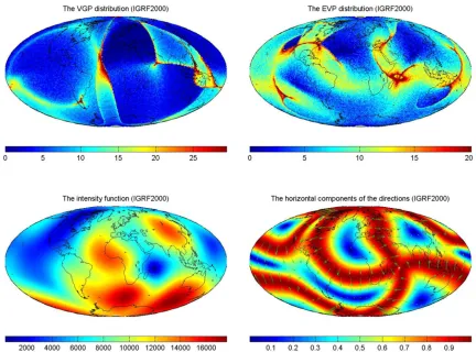
sig-nals of the surface geomagnetic field depicted from the VGP and the EVP distributions of a given paleomagnetic DDS are independent and complementary. To illustrate the cor-relations between the characteristics of the VGP, the EVP distributions and the features of the geomagnetic field in a more practical context, we use here the almost ideal VGP and EVP distributions of the DDSs (the site distribution is al-most ideal) for the individual harmonics (Fig. 1) and for the non-dipole and non-zonal IGRF2000 models (Fig. 2) as the examples. The VGP distributions and EVP distributions for the DDSs of the vector fields containingg1₂andg₂2spherical harmonics respectively are shown in Fig. 1. The VGP distri-bution, the EVP distridistri-bution, the intensity function and the horizontal components of the directions for the non-dipole and the non-zonal IGRF2000 (excluding degree 1 and all zonal harmonic coefficients) are shown Fig. 2. In order to more clearly show the patterns of the VGP and the EVP dis-tributions, the “density” (the populationsper location) of the VGPs and the EVPs shown in Fig. 1 is the natural logarith-mic of the original value (ln[“density”]) and those shown in Fig. 2 is the square root of the original value.

(3)

Fig. 1. The VGP distribution (top panel), the EVP distribution (bottom panel) forg1

2(right column) andg22(left column) spherical harmonics.

(4)

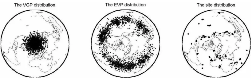
Fig. 3. The VGP (1528 VGPs), the EVP (1528 EVPs) and the site (74 sites) distributions for the lava data set for the past 5 million years, the ﬁgures are the Lambert azimuthal equal-area projections from the north geographic pole with latitudinal parallel extending to 70◦south.

characteristic (e.g. uniform and/or non-uniform) divergences of the directions as they approaching the null ﬂux lines. We do not discuss these high order correlations further, because the matters may be viewed as of less practical interests.

We now summarize the preceding discussions. First, we showed that the VGP distribution and the EVP distribution are essentially two different 2D projections of a 3D DDS on a unit sphere. A paleomagnetic DDS is, in principle, more adequately represented by using both the VGP and the EVP distributions. Second, by using the VGP distribution and the EVP distribution of the single spherical harmonic and the IGRF model as the examples and from other similar simulations over the years, we suggest that:

Proposition 1: The VGP distribution depicts the locations of the poles. The patterns of the VGP distribution illuminate the convergences of the lines of force of the surface geomag-netic ﬁeld as such that the regions of high VGP concentra-tions correlate to the regions where (a) the direcconcentra-tions tend to be more perpendicular to the earth’s surface, (b) the lines of force converge to form the poles and (c) the intensities are generally higher.

Proposition 2: The EVP distribution depicts the locations of the null flux lines. The patterns of the EVP distribution illuminate the divergences of the lines of force of the surface geomagnetic field as such that the regions of high EVP con-centrations correlate to the regions where (a) the directions tend to parallel to the earth’s surface, (b) the lines of force diverge to form the null flux lines and (c) the intensities are generally lower.

Although, in this section, we use the VGP distributions and the EVP distributions of almost ideal DDSs to illustrate the respective roles of the VGP distribution and the EVP dis-tribution in depicting the signals of the geomagnetic field from a DDS, our aims are to use these roles to depict the signals from the DDS with less ideal (or often far less ideal) site distributions. For instance, if the site distribution in a paleomagnetic DDS is sparse but somewhat reasonable, then meaningful patterns of the VGP and the EVP distributions start emerging (for instance, one could obtain the VGP and the EVP distributions that are similar to those in Fig. 2 with about 100 randomly distributed sites). The general locations of (a) the poles and (b) the null flux lines of the surface geo-magnetic field may then be visualized and estimated from the VGP and the EVP distributions respectively, even though the locations of the poles and the locations of the null flux lines

are not (adequately) covered by the sites. Furthermore, since the site distribution in the paleomagnetic DDSs is grossly in-adequate and biased, the combination of the VGP and the EVP distributions (together with the site distribution) can be used not only to depict useful (but often incomplete) signals of the earth’s magnetic ﬁeld but also to evaluate the credibil-ity of the signals due to the inﬂuences of the site distribution which we shall discuss in the following section.

3. The VGP Distribution and the EVP Distribution

of the Paleomagnetic DDS

To illustrate the applications of the EVP distribution in pa-leomagetic analyses, we use two well-known paleomagnetic DDSs, (a) the lava data set for normal polarity of the last 5 million years (Johnson and Constable, 1995) and (b) the Matuyama-Brunhes polarity reversal. The data set (b) is ob-tained from U.S. NOAA and consists of only the transitional directional data during the polarity reversals (deﬁned as VGP latitudes less than±55◦). The VGP and the EVP and the site distributions for the data sets (a) and (b) shown in Fig. 3 and Fig. 5 respectively.

(5)

combined contributions from the longitudinally biased site distribution, the non-axial symmetries, the geocentric axial symmetries and other noises. Therefore, using only the lon-gitudinal uniformity in the VGP distribution (while the site distribution is longitudinally biased), one could not logically conclude the predominance of the geocentric axial symme-tries in the NAD, nor preclude them.

Unlike the VGP distribution, the EVP distribution in Fig. 3 is uneven and discontinuous at the geographic equatorial re-gions. If the site distribution is not taken into account, the overall patterns of the EVP distribution would suggest that the primary conﬁgurations of the earth’s magnetic ﬁeld are not even dipolar but highly non-axial symmetrical. While taking into account of the site distribution, the characteristic patterns in the EVP distribution, such as that the distribution of the EVPs is strongly parallel to the longitudes at many places and longitudinally correlates with the site distribu-tion, imply relatively strong time-dependent geocentric axial symmetries in the DDS. Therefore, for the lava data set for the past 5 million years, the contributions of geocentric axial symmetries obtained from the longitudinal biased EVP dis-tribution vs. the longitudinal biased site disdis-tribution is more obvious than those obtained from the longitudinal uniform VGP distribution vs. the longitudinal biased site distribution. Taking the estimates that are consistent with both the VGP and the EVP distributions vs. the site distribution, one could then logically conclude a strong presence of the geocentric axial symmetries in the DDS.

As we noted earlier, in theory the VGP distribution and the EVP distribution are equally important. For a purely geocen-tric axial symmegeocen-trical DDS, they are also equivalent. But, the geocentric axial symmetries in the lava data set for the past 5 million years are much better illustrated in the EVP distribution (together with the site distribution) than in the VGP distribution. This is because the VGP distribution and the EVP distribution are in the sense two different (2D) ways of “wrapping up” all of the signals in the 3D DDS (including the directions, the noise and the site distribution). For the lava data set for the past 5 millions years, the signals of the geocentric axial symmetries are obscured as all of the signals in the DDS being wrapped (projected) into the VGP distri-bution, but they are not obscured in the EVP distribution. Of course, in other cases, it may be that the contaminations in the EVP distribution are stronger than those in the VGP distribution. Therefore, we suggest, in order to obtain the optimal characteristics of the geomagnetic ﬁeld from a pale-omagnetic DDS, both the VGP distribution and the EVP dis-tribution (together with the site disdis-tribution) should be used. 3.2 The clariﬁcation of a paleomagnetic DDS

Because of the grossly inadequate and biased site distri-bution in a paleomagnetic DDS, it is important in the paleo-magnetic analyses to evaluate the influences of the site dis-tribution. Obviously, the influences of the site distribution in a DDS cannot be evaluated by using the values of the decli-nations and the inclidecli-nations commonly used to represent the directions, because these values cannot be directly compared with the locations of the sites. Also, the influences of the site distribution cannot be evaluated by inspecting only the site distribution because the site distribution does not con-tain and is not related to any information on the directions

(although the inadequate and the biased site distribution may suggest the suspicions).

We suggest that, by representing the DDSs in terms of the VGP distribution and the EVP distribution, the influences of the site distribution in the DDS can then be assessed by com-paring three point distributions—the VGP distribution, the EVP distribution and the site distribution. If either the EVP distribution or the VGP distribution (or both) is correlated with the site distribution, then these correlations in turn sug-gest the influences of the site distribution in the DDS. Here, we define a paleomagnetic DDS as,

(A) a “local” DDS and the signals depicted from the “lo-cal” DDS are “localized” signals, if the VGP distribution and/or the EVP distribution are correlated with the site dis-tribution.

For instance, the mean longitudinal distance (|EVP Lon.– Site Lon.|) in Fig. 3 is 8.24◦ and its standard deviation is 13.94◦ (the mean distance of |VGP Lon.–Site Lon.| is 101.42◦ and its standard deviation is 47.22◦). Therefore, the longitudinal distribution of the EVPs roughly follows the longitudinal distribution of the sites (the longitudinal distri-bution of the VGPs is not correlated with the longitudinal distribution of the VGPs). It is also easy to identify that the longitudinal locations of the ‘gaps’ in the EVP distribution are correlated with the ‘gaps’ in the site distribution. The longitudinal correlations between the EVP distribution and the site distribution suggest that the lava data set for the past 5 million years in Fig. 3 is inﬂuenced by the site distribution. Therefore, it is a “local” DDS and the signals depicted from it are “localized” signals.

(B) A “presumed global” DDS and the signals depicted from the “presumed global” DDS are the “presumed global” signals, if the VGP distribution and the EVP distribution are uncorrelated with the site distribution (or the correlations can not be established).

The inﬂuences of the site distribution can be evaluated in the “local” DDS, but they cannot be evaluated in the “presumed global” DDS (even though the “presumed global” DDS may also be inﬂuenced by the site distribution).

(6)

Fig. 4. The VGP and the EVP distributions for 3 TAF models: the VGP and the EVP distributions are computed by using all of the original gauss coefﬁcients of 3 models, except thatg0

1, are reduced to 50% of their original values, the ﬁgures are the Lambert azimuthal equal-area projections from the north geographic pole with latitudinal parallel extending to 70◦south.

Fig. 5. The VGP distribution (green), the EVP distribution (blue) and the site distribution (red) for the Matuyama-Brunhes reversal.

3.3 The inﬂuences of the site distribution in the time-averaged ﬁeld models

The site distribution may also influence the models of the earth’s magnetic field inverted from a “local” paleomagnetic DDS. The methods of evaluating the influences of the site distribution are as follows: we first depict the correlations be-tween the original VGP distribution (the original EVP distri-bution) and the site distribution of a paleomagnetic DDS. We then obtain the VGP distribution (the EVP distribution) pred-icated by the inverted model of the earth’s magnetic field. Fi-nally, if the predicated VGP distribution (the predicated EVP distribution) is also correlated with the original VGP distri-bution (the original EVP distridistri-bution), then the signals in the inverted model are obviously influenced by the site distribu-tion. If there are no such correlations, then the signals are presumably not influenced by the site distribution.

We use 3 different the time-averaged field (TAF) models for past 5 millions years as the examples to illustrate the methods. These models are inverted by 3 different groups using different inversion methods and are published over the last 7 years. The data sets used are almost the same as the lava data set of the past 5 million years shown in Fig. 3 (in fact, two of them are actually used the same DDS in Fig. 3). We first compute a DDS for each TAF models on an almost ideal site distribution by using the original coefficient of the model with g0₁ being reduced to 50% of its original value. (This reduction of g₁0 is to help graphically enhancing the patterns in the EVP distributions due to the non-axial-dipole contributions in TAF models.) A VGP distribution and an

EVP distribution predicated by the model are then computed from each DDS. The VGP distributions and the EVP distri-butions predicted by three TAF models are shown in Fig. 4. (The general characteristics of the longitudinal distribution of EVPs in Fig. 4 are similar to those in the EVP distribu-tions generated without reduction ing0

1.) Next, we compare the predicated EVP distributions in Fig. 4 with the original EVP distribution in Fig. 3. The longitudinal variation of the EVP “density” in the predicted EVP distributions in Fig. 4 seems to be qualitatively correlated with that in the original EVP distribution in Fig. 3. In particular, (a) along the equato-rial regions in the vicinities of the longitude 90◦E, the diffuse patterns and the lower average EVP “density” in the predi-cated EVP distributions correlate with the lower concentra-tions of the original EVPs in the same regions, (b) along the equatorial regions roughly west of the longitude 90◦W and roughly in the vicinities of the longitude 180◦, the lower av-erage EVP “density” in the predicated EVP distribution also correlates with the lower concentrations of the original EVPs in these regions. (c) Along the equatorial regions in the vicin-ity of the prime meridian and, to a lesser extent, in the regions extending from the west of longitude 90◦W to the longitude 180◦, the predicted EVPs are relatively densely distributed within the approximate arcs. The relatively higher average EVP “density” in the predicated EVP distribution correlates with the high concentrations of the original EVPs in the same regions.

(7)

Fig. 3 which in turn longitudinally correlates with the site distribution in Fig. 3 as discussed previously suggest that at least parts of the NAD contribution predicted by three TAF models are influenced by the inadequate and the biased site distributions. The correlations between the predicated EVP distributions and the original EVP distribution probably re-sulted from the fact that, in the processes of fitting the orig-inal directions in the DDS, the TAF models also inevitably tend to fit the original EVP distribution (because it represents parts of the information in the DDS). Consequently, the TAF models interpret the longitudinal variations in the original EVP distribution as signals of the earth’s magnetic field (in spite of the fact that one model uses a so-called “smooth-ness” constraint in an attempt to minimize the structures in the TAF model), but in fact they are the artifacts due to the inadequate and biased site distribution.

In view of the preceeding discussions on the influences of the site distribution, we suggest that the caution should be taken in interpreting these features. In particular, the esti-mates on the non-zonal contributions of the NAD in three TAF models are easily influenced by the artificial longitu-dinal variations of the EVP distribution. Furthermore, the broad similarities in longitudinal variations of the EVP dis-tributions shown in Fig. 4 also imply that there are similar features in the morphologies of three TAF models. These features are often interpreted as the persistent NAD contri-butions of the earth’s magnetic fields because they appear in different TAF models (whereas the differences in patterns of the TAF models are often attributed to the different methods used in the inversions). In fact, the features that repeatedly appear in different TAF models are not necessarily the per-sistent NAD contributions of the earth’s magnetic field, be-cause the influences of the site distribution always exist and may also appear as persistent features in these models (if the models are inverted from similar data sets), irrespective of whatever the inversion methods are used. It is interesting to note that some of the persistent patches (such as those in the Siberia region) in the morphologies of three TAF models are located within the longitudinal bands where the average EVP “density” is lower in both the predicted EVP distribution and the original EVP distribution.

3.4 The EVP distribution for the Matuyama-Brunhes polarity reversal data set

The EVP distribution during the polarity transition in Fig. 5 follows the site distribution. The most distinctive cor-relations between the EVP and the site distributions are their respective populations in the northern and the southern hemi-spheres, and the higher population of the EVPs in the Paciﬁc region correlates with the higher concentrations of the sites there. The mean distance between the EVPs and the cor-responding sites is about 2◦ with standard deviation of 25◦. (Note: as the inclination decreases, the EVP approaches the site. When inclination is zero, the EVP is located at the site.) Shallow inclinations during the transitional periods of the po-larity reversal are sometimes attributed to the depositional errors in the sedimentary records. However, it can be shown by plotting the EVPs of the individual record that, irrespec-tive of whether it is the lava, the oceanic, or the sedimentary record, the EVPs has a pattern of clustering about the site with no azimuth preferences. These characteristic shallow

inclinations also do not depend upon the geographic loca-tions of the sites. Therefore, we suggest that the “shallow inclination” effect is the characteristic signal of the earth’s magnetic ﬁeld during transitional period of the polarity re-versal.

The patterns in the corresponding VGP distributions in Fig. 5 are interpreted to be preferred VGP paths along the America continent and East Asia (Clement, 1989; Lajet al., 1991) and clusters of VGPs (Hoffman, 1996), but these ideas are contested by others (Prevot and Camps, 1993). Follow-ing our previous discussions, the preferred VGPs paths and clusters of VGPs illuminate the locations of the persistent poles of the earth’s magnetic field during the transitional pe-riod of the polarity reversals. The EVP distribution following the distribution of the sites (the “shallow inclination” effect) suggests the absences of the persistent null flux lines of the earth’s magnetic field in the observations during the same pe-riod. Of course, given the site distribution, we have reasons to attribute the absences of the persistent null flux lines in the EVP distribution to the inadequate spatial samplings of the reversal records. But in the interests of motivating future analyses of the polarity reversal data set, we wish to spec-ulate that if the EVP distribution does indeed follows the site distribution, then it would imply that there are persis-tent poles but without the corresponding persispersis-tent null flux lines in the earth’s surface magnetic field during the transi-tional period of the polarity reversals. This kind of surface morphologies may not be plausibly explained as due to the physical processes (or the physical conditions) taking place entirely beneath the earth’s surface (such as those suggested by the hypothesis of the mantle and the core-mantle bound-ary controls). Therefore an important and interesting point in the future analyses on the DDSs of the polarity reversals is to determine the persistent null flux lines from the EVP distribution as new reversal records becoming available.

(8)

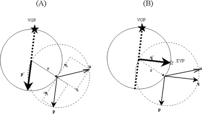
Fig. 6. The graphic constructions of (A) the VGP and (B) the EVP, the ﬁgures represent views on the great circles passing through the siterˆin the direction ofuˆ(rˆ).

3.5 Summary

In this section, we summarize and generalize the previ-ous discussions on the applications of the VGP distribution and the EVP distribution in the paleomagnetic analyses: (1) By using the lava data set for the past 5 million years, we demonstrated that the estimates obtained from only the VGP distribution are sometimes ambiguous. Of course, there are other similar cases in paleomagnetic studies. For instance, it has been known for sometimes that, in the paleomagnetic reconstructions of the continents and the plates, estimating a paleo-pole from only the VGP distribution (e.g. the mean VGP) is sometimes ambiguous and uncertain, probably due to the persistent non-dipole contributions. We suggest that any optimal characteristics of the geomagnetic field obtained from a paleomagnetic DDS (such as the paleo-pole) should be the “best-fittings” to both the VGP and the EVP distribu-tions (Note: the statistical characteristics of the VGP bution are generally different from those of the EVP distri-bution). (2) We clarified a paleomagnetic DDS as a “local” DDS, if either the VGP distribution or the EVP distribution (or both) is correlated with the site distribution; and as a “pre-sumed global” DDS, if there are no such correlations. We suggested that, for a “local” DDS, the influences of the site distribution in the paleomagnetic DDS and in the models in-verted from it can be evaluated. The influences of the site distribution cannot be detected (even though they do exist), if the original paleomagnetic DDS is a “presumed global” data set. (3) We showed that the VGP distribution and the EVP distribution could be helpful in respectively evaluating the locations of the poles and the locations of the null flux lines in cases that the site distribution in a paleomagnetic DDS does not (adequately) cover these locations. Further-more, because the positioning of the sites with respect to the field structure is always unknown, it is also possible that in some cases the sites may be positioned in favor of detecting the locations of the poles, whereas in other cases the sites may be positioned in favor of detecting the locations of the null flux lines. Therefore, in order to at least avoid missing the useful signals or being misled by the artificial features,

we suggested that both the VGP and the EVP distributions should be used under all circumstances.

4. Conclusion

We suggest that the VGP distribution and the EVP dis-tribution are two different 2D projections of a 3D DDS on the earth’s surface (except when the DDS is of the 2D axial symmetrical), therefore using only one of them is insuffi-cient to represent a 3D DDS. Furthermore, comparing with the other representations, the representation of the VGP dis-tribution and the EVP disdis-tribution for a 3D DDS is perhaps interesting in its own right. First, it reduces the 3D directions emanating from the earth’s surface to two 2D point distribu-tions on the same surface. Second, the characteristics of the VGP and the EVP distributions are remarkably associated with some of the primary characteristics of the geomagnetic field. For instance, we show that the VGP distribution and the EVP distribution illuminate from a DDS two sets of the signals with complementary characteristics: the locations of the poles and the locations of the null flux lines. The loca-tions of the poles are emphasized by the high concentraloca-tions of the VGPs and the null flux lines are emphasized by the high concentrations of the EVPs.

We suggest that both the VGP distribution and the EVP distribution (together with the site distribution) should al-ways be used in the paleomagnetic analyses in order to, (1) obtain both the locations of the poles and the locations of the null flux lines from a paleomagnetic DDS, (2) reduce the ambiguity in the analyses, (3) evaluate the possible influ-ences of the site distribution in a DDS and in the models of the earth’s magnetic field inverted from a ‘local’ DDS and (4) guide the selections of new sites aiming at reducing the influences of the site distribution. However, we also wish to point out that one of the alternatives to the introduction of the EVP distribution is by labeling the VGP and the corre-sponding site with the same number. This alternative does not appear being feasible in the analyses.

(9)

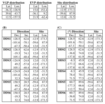
Table 1. The artiﬁcial example, (A) The lists of a VGP distribution, a EVP distribution and a site distribution, (B) The DDSs sharing the same VGP distribution and the site distribution and (C) The DDSs sharing the same EVP distribution and the site distribution.

(A)

VGP distribution EVP distribution Site distribution

Lat. Lon. Lat. Lon. Lat. Lon.

-36.3 -128.9 15.0 152.4 -12.9 -173.3 39.6 -43.7 -36.1 9.2 -59.6 87.9 12.5 -157.5 21.9 -62.4 12.0 -31.5

(B) (C)

Direction Site (*) Direction Site

Dec. Inc. Lat. Lon. Dec. Inc. Lat. Lon. DDS1 128.5 62.6 -12.9 -173.3 DDS1 128.5 62.6 -12.9 -173.3 -101.6 -70.1 -59.6 87.9 -101.6 -70.1 -59.6 87.9 -67.3 -50.4 12.0 -31.5 -67.3 -50.4 12.0 -31.5 DDS2 128.5 62.6 -12.9 -173.3 DDS2 128.5 62.6 -12.9 -173.3 -19.3 74.1 12.0 -31.5 -36.8 74.8 12.0 -31.5 105.1 -40.4 -59.6 87.9 -137.8 61.9 -59.6 87.9 DDS3 -124.9 -24.8 12.0 -31.5 DDS3 -8.3 45.9 12.0 -31.5 49.2 -57.8 -12.9 -173.3 -177.3 66.6 -12.9 -173.3 105.1 -40.4 -59.6 87.9 -137.8 61.9 -59.6 87.9 DDS4 -124.9 -24.8 12.0 -31.5 DDS4 -8.3 45.9 12.0 -31.5 -101.6 -70.1 -59.6 87.9 78.4 70.1 -59.6 87.9 32.3 74.0 -12.9 -173.3 71.5 77.5 -12.9 -173.3 DDS5 150.5 20.5 -59.6 87.9 DDS5 60.7 89.6 -59.6 87.9 49.2 -57.8 -12.9 -173.3 -177.3 66.6 -12.9 -173.3 -67.3 -50.4 12.0 -31.5 112.7 50.4 12.0 -31.5 DDS6 150.5 20.5 -59.6 87.9 DDS6 60.7 89.6 -59.6 87.9 -19.3 74.1 12.0 -31.5 -36.8 74.8 12.0 -31.5 32.3 74.0 -12.9 -173.3 71.5 77.5 -12.9 -173.3

Note: (*) means that every direction listed in the table and its opposition has the same EVP

the past 5 million years are at least partly influenced by the longitudinal distribution of the site and (b) the morphologies of geomagnetic field during the transitional period of the Matuyama-Brunhes polarity reversal are characterized by the persistent locations of the poles (emphasized by the preferred distributions of the VGPs) without the persistent null flux lines (“the shallow inclination effect” suggested by the EVP distribution). Obviously, new paleomagnetic data are needed to improve the present understanding on the time-averaged behaviors and the polarity reversals of the earth’s magnetic fields.

Acknowledgments. One of us, Shao Ji Cheng wishes to acknowl-edge the support by JSPS postdoctoral fellowship from the gov-ernment of Japan. This work has beneﬁted from the discussions with Prof. Mike Bevis and Prof. Fred Duennerbier of University of Hawaii at Manoa.

Appendix A. The Geometrical Constructions of the

VGP and the EVP from Direction

The VGP and the EVP can be constructed by using the geometric methods as follows: a directionuˆ(rˆ)at the siterˆ consists of the radial componentur, perpendicular to the unit

sphere and the horizontal componentustangential to the unit

sphere. To obtain the VGP foruˆ(rˆ), we ﬁrst draw at the site

ˆ

ra vectorpgiven by,

p=0.5urrˆ−us. (A.1)

We then normalizep to obtainpˆ and draw from the center of the unit sphere a unit vector pˆ parallel topˆ. The point of intersection between pˆ and the unit sphere is the VGP ofuˆ(rˆ)as shown in Fig. 6(A). To obtain the corresponding EVP fromuˆ(rˆ)andrˆ, we draw from the center of the sphere the unit vector qˆ, which is perpendicular to pˆ and lies in the plane defined by pˆ and the site vectorrˆ as shown in Fig. 6(B). Theoretically, there are two such vectors, but we choose the one making an angle withrôf less than 90◦. We then define the “equatorial virtual pole” (EVP) as the point of intersection between the unit vectorqând the unit sphere as shown in Fig. 5(B). Similar to calculating the vectorpin Fig. 5(A), the vectorqwhich is drawn at site and parallel to

ˆ

q(and the EVP) in Fig. 5(B) can also be calculated from the directional datauˆ(ˆr)and the siterˆas,

q=(1−u2r)rˆ−0.5urus. (A.2)

(10)

case, the EVP can no longer be defined as a pole, but degen-erate to a great circle 90◦from the site. A VGP and an EVP can be uniquely determined from a direction on the earth’s surface. From the traditional standpoint of the dipole con-cept used for interpreting the VGP (e.g. Merrillet al., 1996), the EVP corresponds to a point on the equator of a dipole placed at the center of the earth that generates the observed direction at the site. However, our discussions show that the VGP and the EVP can be used to represent any direction. It is interesting to note that there are infinite pairs of the or-thogonal unit vectors (and infinite pairs of the corresponding point distributions) which can be similarly defined foruˆ(rˆ). It appears that only the pair ofpˆ andqˆ defined here and the corresponding VGP and EVP distributions show the remark-able properties. The reason for this is not clear.

Appendix B. An Artiﬁcial Example

We suppose that a VGP distribution, an EVP distribution and a site distribution are given as listed in Table 1(A) (with-out any correlations attached to the three distributions). How many sets of DDS generated the same VGP and the site dis-tribution in Table 1(A)? The answer is six sets of different DDSs as listed in Table 1(B), but ﬁve of them generate the EVP distributions different from that listed in Table 1(A). Given an EVP distribution and a site distribution, only the unsigned directions can be determined. The DDSs with the declinations, the inclinations and the sites listed in Table 1(C) share the same EVP distribution and the site distribu-tion listed in Table 1(A). But only one of them has the same VGP distribution in Table 1(A). Comparing the DDSs in Ta-bles 2(B) and (C), there is only one DDS (DDS1 in TaTa-bles 1(B) and (C)) which has the same VGP distribution, EVP distribution and the site distribution in Table 1(A).

References

Clement, B., Longitudinal distribution of Brunhes-Matuyama transitiona VGPs,EOS Trans. AGU,70, 1073, 1989.

Courtillot, V., J.-P. Valet, G. Hulot, and J. L. Le Mou¨el, The Earth’s magnetic ﬁeld: Which symmetry,EOS Trans. AGU,73, 337, 340–342, 1992. Gubbins, D. and P. Kelly, On the analysis of paleomagnetic secular

varia-tion,J. Geophys. Res.,100, 14,955–14,964, 1995.

Hoffman, K. A., Transitional paleomagnetic ﬁeld behaviour: Preferred paths or patches,Surv. Geophys.,17, 207–211, 1996.

Hatakeyama, T. and M. Kono, Geomagnetic ﬁeld model for the last 5 My: time-averaged ﬁeld and secular variation,Phys. Earth Planet. Inter.,133, 181–215, 2002.

Johnson, C. L. and C. G. Constable, The time-averaged ﬁeld as recorded by lava ﬂows over the past 5 Myr years,Geophys. J. Int.,122, 489–519, 1995.

Laj, C. A., A. Mazaud, R. Weeks, M. Fuller, and E. Herrero-Bervera, Geo-magnetic Reversal Paths,Nature,351, 447, 1991.

Merrill, R. T., E. W. McElhinny, and P. L. McFadden,The Magnetic Field of the Earth,Academic Press, 1996.

Prevot, M. and P. Camps, Absence of preferred longitude sectors for poles from volcanic records of geomagnetic reversals,Nature,366, 53–57, 1993.

Quidelleur, X., J.-P. Valet, V. Courtillot, and G. Hulot, Long term geometry of the geomagnetic ﬁeld for the last ﬁve million years,Geophys. Res. Lett.,21, 1639–1642, 1994.

Shao, J.-C., M. Fuller, T. Tanimoto, J. R. Dunn, and D. B. Stone, Spherical Harmonic analysis of Paleomagnetic Data: The time-averaged geomag-netic ﬁeld for the past 5 Myr and the Matuyama-Brunhes Reversal,J. Geophys. Res.,104, 5015–5030, 1999.

Shao, J.-C. and M. Fuller, Hemispherical Asymmetry in reversal Transition Fields, IUGG XXII, Abstracts, A292, 1999.

Shao, J.-C. and Y. Hamano, Inferences of the earth’s magnetic ﬁeld from surface directional data, pp. 171, Proceedings of the OHP/ION Joint Symposium, 2001.

Shao, J.-C., Y. Hamano, M. Bevis, and M. Fuller, A representation func-tion for the point distribufunc-tion on the unit sphere—with applicafunc-tions to the analyses on the distribution of the virtual geomagnetic poles,Earth Planets Space,55(7), 395–404, 2003.