Use of the Comprehensive Inversion method for
Swarm
satellite data analysis
Terence J. Sabaka1, Lars Tøffner-Clausen2, and Nils Olsen2
1Planetary Geodynamics Laboratory, NASA Goddard Space Flight Center, Greenbelt, Maryland, USA 2National Space Institute, Technical University of Denmark, Lyngby, Denmark
(Received March 27, 2013; Revised September 6, 2013; Accepted September 9, 2013; Online published November 22, 2013)
An advanced algorithm, known as the “Comprehensive Inversion” (CI), is presented for the analysis ofSwarm
measurements to generate a consistent set of Level-2 data products to be delivered by theSwarm “Satellite Constellation Application and Research Facility” (SCARF) to the European Space Agency (ESA). This new algorithm improves on a previously developed version in several ways, including the ability to process ground-based observatory data, estimation of rotations describing the alignment of vector magnetometer measurements with a known reference system, and the inclusion of ionospheric induction effects due to ana priori3-dimensional conductivity model. However, the most substantial improvements entail the application of a mechanism termed “Selective Infinite Variance Weighting” (SIVW), which mitigates the effects of non-zero mean systematic noise and allows for the exploitation of gradient information from the low-altitudeSwarmsatellite pair to determine small-scale lithospheric fields, and an improvement in the treatment of attitude error due to noise in star-tracking systems over previously established methods. The advanced CI algorithm is validated by applying it to synthetic data from a full simulation of theSwarmmission, where it is found to significantly exceed all mandatory and most target accuracy requirements.
Key words: Swarm, Earth’s magnetic field, comprehensive modeling, core, lithosphere, ionosphere, magneto-sphere, electromagnetic induction.
1.
Introduction
The European Space Agency (ESA) is scheduled to launch theSwarmmission (Friis-Christensenet al., 2006) in 2013, a constellation of three satellites to map the Earth’s magnetic field to unprecedented accuracy. During its multi-year lifetime, two low orbiting spacecraft will act as a mag-netic gradiometer while a third at higher altitude monitors the main and external fields at other local times. ESA has established theSwarm“Satellite Constellation Appli-cation and Research Facility” (SCARF) for the purposes of generating derived Level-2 products from the single-satellite Level-1b data. The “Comprehensive Inversion” (CI) method of Sabaka and Olsen (2006) is a major process-ing chain of SCARF, producprocess-ing one version of each of five defined items: core, lithospheric, magnetospheric, and iono-spheric iono-spherical harmonic expansions, time-varying when appropriate, and Euler angles describing the alignment be-tween the vector fluxgate magnetometer frame (VFM) tem and that of the Common Reference Frame (CRF) sys-tem of the star imager.
The basic CI algorithm is presented in Sabaka and Olsen (2006) where the magnetic fields from all major near-Earth current sources are parameterized and then co-estimated to obtain optimal field separation. This co-estimation ap-proach is the key to the superior results obtained because it eliminates ambiguities between parameters spaces.
Tech-Copyright cThe Society of Geomagnetism and Earth, Planetary and Space Sci-ences (SGEPSS); The Seismological Society of Japan; The Volcanological Society of Japan; The Geodetic Society of Japan; The Japanese Society for Planetary Sci-ences; TERRAPUB.
doi:10.5047/eps.2013.09.007
nically, the basic CI algorithm is an iterative Gauss-Newton (GN) least-squares estimator (Seber and Wild, 2003), which derives the model parameters from Swarmvector magne-tometer measurements. While its application to theSwarm
E2E simulator (Sabaka and Olsen, 2006) showed promis-ing performance in field recoverability, it still lacked several features that would render it a truly competent algorithm for the generation of actual Level-2 products. For instance, the basic algorithm did not allow for surface measurements such as observatory hourly-means (OHM) data, which are known to greatly enhance field separation. Estimation of the rotation between the VFM and CRF system for vector measurements mentioned above was not included in the ba-sic algorithm. The a priori conductivity model assumed for ionospheric induction was 1-dimensional (1D) rather than 3-dimensional (3D) in its variation. Finally, the formal treatment of measurement and theory errors was very prim-itive and not considered versatile enough for actual mission application.
In this paper an attempt will be made to remedy the aforementioned inadequacies of the basic algorithm by de-veloping an advanced CI algorithm. While this new algo-rithm now admits the OHM data, estimates the Euler angles describing the VFM to CRF rotations, and includes iono-spheric induction due to 3D conductivity structure, its great-est advancement is in the area of formal error treatment. Here a methodology, termed “Selective Infinite Variance Weighting” (SIVW), is developed to handle non-zero mean error due to, for instance, theory inadequacies through the use of bias estimation which exploits Signal-to-Noise ratio (SNR) levels in different data subsets in order to extract the
best models. In addition, the methodology of Holme and Bloxham (1995, 1996) and Holme (2000) to account for at-titude error present in vector magnetometer measurements due to star tracker instabilities is revised in order to improve parameter estimates in the CI algorithm. The entire error treatment mechanism is then placed in the context of robust estimation by applying a Huber weighting scheme to mit-igate the effects of outliers (Constable, 1988; Walker and Jackson, 2000; Olsen, 2002).
The structure of the paper is as follows: a brief overview of the basic CI algorithm will be presented in Section 2, followed by the development of SIVW in Section 3. In Section 4 the improved attitude error framework will be derived, followed by the development of the advanced CI algorithm in Section 5. The results of the application of the advanced algorithm to synthetic data from a mission simulation, known as “Version-2” (V2) (Olsenet al., 2013), and a discussion are in Section 7, followed by conclusions in Section 8. Finally, Appendices A and B are provided that contain some technical information and derivations of formulae presented in Sections 4 and 5, respectively.
2.
Overview of the Basic CI Algorithm
The basic CI algorithm essentially employs the same field source parameterizations as the CM4 model of Sabaka
et al. (2004), except for the magnetosphere and its asso-ciated induced field. These latter fields were rather dis-cretized in contiguous bins through time and considered static within each bin. The magnetospheric and associated induced fields are modeled independently with the intent of discovering something of the underlying conductivity struc-ture in Earth’s outer shell. These overall parameterizations have been presented in Sabaka and Olsen (2006) where spe-cific details may be found. However, a synopsis of this pa-rameterization is given in Table 1, where the spherical har-monic (SH) expansions begin at degree 1 and are truncated at maximum degree/orderNmax/Mmax.
Because the induced field associated with the magneto-sphere is modeled as an internal field to full degree/order 3, it can mimic the internal core field as its bin duration de-creases. As a consequence, separation of induced fields at periods longer than, say, a few months from rapid core field changes is not possible. This happens even though the in-duced field is expressed in dipole SH functions while the core is in geographic. This means that co-linearity poten-tially exists between the parameters of these two fields. To alleviate this, the basic CI algorithm employs equality con-straints that force point-wise orthogonality over the mea-surement times between any linear functionals of the core and induced SH parameters. This will be derived again in this paper for clarity. Let
ζc(r,t)=Tc(r)pc(t)=Tc(r)Pcbc(t), (1)
ζi(r,t)=Ti(r)pi(t)=Ti(r)Pibi(t), (2)
where the subscript “c” and “i” indicate core or induced fields, respectively, and ζ(t,r) is the linear functional at time t and position r, (r) is the SH linear mapping at positionr,p(t)is the vector of SH coefficients at timet,Pis the matrix of temporal coefficients for each SH coefficient
such that(P)i j is the j-th temporal coefficient for the i
-th SH coefficient, andb(t)is the vector of temporal basis functions at timet. Specifically, the first element ofbc(t) is a one (for the static term) followed by a series of B-spline terms defined over the time domain of the model, whilebi(t)is of lengthNb(the number of time bins for the induced field) with a one in the position of the bin wheret
resides and zeros elsewhere. The objective is to make the following summation vanish over the set of measurement timest1, . . . ,tNm
A more convenient form is realized by stacking the Ni columns ofPT
i (or the Ni rows ofPi) to make a vectorιιι, which itself is a sub-vector of the parameter vector for the entire modelx, so that
¯
Gx=0. (5)
Ifbc(t)is of lengthNc, thenG¯ is a sparse matrix containing the appropriate pattern ofGsuch that itsNc·Nirows enforce a like number of constraints specified in Eq. (4) when multi-plyingx. Therefore, it is Eq. (5) that is used to constrain the least-squares solution so that the induced magnetospheric field is subjugated to the core field to be point-wise orthog-onal to it over the measurement times. Because the core spline basis is broad-scale in time, this means thatιιι will reflect more high-frequency behavior in the internal field, which is reasonable for much of the induced effects.
The result is that the basic CI algorithm solves the follow-ing least-squares problem with linear equality constraints (LSLE) at thek-th GN step (LSLE-GN)
LSLE-GN
are the residuals of the data vectord with respect to the non-linear model vectora(xk)evaluated atxk,Ak ≡A(xk)
is the Jacobian of the model vector evaluated at xk,xk
are the adjustments to the current parameter vectorxk,Lis
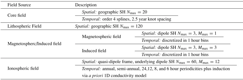
Table 1. The basic CI source parameterization (Sabaka and Olsen, 2006).
Field Source Description
Core field Spatial:geographic SHNmax=20
Temporal:order 4 splines, 2.5 year knot spacing Lithospheric Field Spatial:geographic SHNmax=120
Magnetospherc/Induced field
Magnetospheric field Spatial:dipole SHNmax=3,Mmax=1
Temporal:discretized in 1 hour bins Induced field Spatial:dipole SHNmax=3,Mmax=3
Temporal:discretized in 1 hour bins Ionospheric field
Spatial:quasi-dipole frame, underlying dipole SHNmax=60,Mmax=12
Temporal:annual, semi-annual, 24,12, 8, and 6 hour periodicities plus induction viaa priori1D conductivity model
C = LLT, and F
j is the square-root factor of the j-th a priori covariance matrixP−j1 = FjFTj that, along with
the Lagrange multiplier λj, specifies the deviation of the
solution from the preferreda priorimodel vectorxj. The
solution to LSLE-GN, denotedxk, may be found through
Lagrange multiplier theory (Toutenburg, 1982; Golub and van Loan, 1989; Bertsekas, 1999) to be
xk=xk−E−k1G¯
TGE¯ −1
k G¯
T−1G¯x
k+xk
, (7)
whereEk = ATkC−1Ak+
Nq
j=1λjPj, andxk is the
un-constrained solution given by
xk =E−k1
ATkC−1dk+ Nq
j=1
λjPj
xj−xk
. (8)
Note that only the linear LSLE-GN was discussed in Sabaka and Olsen (2006). In practice, the Nq quadratic norms in
Eq. (6) are smoothing terms whose preferred solutions are zero, that is, xj = 0. These smoothing norms affect the secular variation of the core field, conductivity structure of the ionospheric E-region, polar gaps, etc., and will be discussed briefly in Section 5.4.
What is not included in the basic CI is a mechanism to exploit the enhanced lithospheric SNR in the differences of the vector measurements made by theSwarmlow satellite pair. It is more complicated than simply using only the low pair vector differences to make models since the comple-mentary data set (the low pair vector sums) is needed in order to resolve other field constituents. In the next section such a mechanism is indeed developed. The application of this mechanism toSwarmwill be discussed in Section 5.
3.
Selective Infinite Variance Weighting
The near-Earth magnetic field is a highly dynamic sys-tem containing signals that vary over a large range of spatial and temporal scales. Even a constellation likeSwarm can-not completely decouple all of the space and time modes. A prominent example is the mis-modeling of time-varying external fields which can manifest itself as spurious static structure, for instance, in the lithospheric field. While this structure may be spatially broad-scale, it can vary rapidly in time and represents a systematic noise bias that can con-taminate the nominal estimate of the lithospheric field. Dif-ferent philosophies exist on how to enhance the recovery
of signals of interest, like the lithosphere, while mitigating the effects of unwanted or contaminating signals in the es-timation procedure. Several recent models have employed direct data selection techniques to derive good descriptions of core and crustal fields (Mauset al., 2007, 2008; Thom-son and Lesur, 2007; Lesuret al., 2008; Olsenet al., 2011). The “Comprehensive Modelling” (CM) approach (Sabaka
et al., 2002, 2004) has not generally relied upon this prac-tice, with the exception of gross outliers, etc., but rather has focused on using as much data as possible to ensure a stable co-estimation of parameters from all sources. Comparison of the CMs with these models, however, has revealed effects of contamination, particularly of ionospheric “leakage” into lithospheric fields.
TheSwarmconstellation offers the ability of taking dif-ferences between the vector magnetometer measurements of the satellite low pair, which effectively eliminates most of the broad-scale external contamination, thus leading to a high SNR of the crustal field signal. However, the comple-mentary data set, i.e., the summation of the vector magne-tometer measurements of the satellite low pair, is necessary for a full co-estimation of the other field constituents, but it has a much lower SNR for its lithospheric field because it suffers from the aforementioned systematic noise bias. With this in mind, a more sophisticated error treatment will be required of the CI models in order to exploit the high SNR in one data set while limiting damage done by retain-ing low SNR data. The SIVW mechanism is now developed by first showing its ability to eliminate bias from system-atic noise of a particularly common form that would oth-erwise contaminate estimates if treated in traditional ways, and secondly, how to combine this property with selection of data subsets that exhibit different SNRs for different pa-rameter sets in order to obtain optimal solutions.
3.1 Mitigating biases
subspaces due to the fact thatq =dim(z) > p=dim(y). Consider the following model
d=Ax+ννν, (9)
=A B x
y
+ηηη, (10)
in which a vector of parameters of interestxare related to a vector of measurementsdthrough a linear operatorAin the presence of an additive error termννν=z+ηηη, wherezis the systemic error defined previously andηηη∼N(0,C)is a random error independent ofzsuch thatννν ∼ N(Bμμμ,C+ BQBT). If a zero-mean assumption is made aboutννν, then the data noise weight matrix will be given by
W=C+BQBT−1, (11)
and the least-squares estimate ofxwill be
˜x=x+ATWA−1ATW(By+ηηη) , (12)
but this is a biased estimate since E[˜x−x] =
ATWA−1ATWBμμμ, where E[·] is the expectation oper-ator.
Now consider the case in whichyis treated as determin-istic rather than stochastic and is co-estimated withxgiving
The partitioned solution forxmay be written as
˜x=ATW∞A−1ATW∞d, (14)
=x+ATW∞A−1ATW∞(By+ηηη) , (15)
=x+ATW∞A−1ATW∞ηηη, (16)
where
W∞=C−1−C−1BBTC−1B−1BTC−1. (17)
Thus,W∞B = 0 and the estimate is now unbiased since
E[˜x−x]=0. In this case,yis treated as a vector of “nui-sance” parameters that are co-estimated with the nominal parametersxin order to absorb error biases. IfQis rewrit-ten as Q = σ2Q¯ and Win Eq. (11) is expanded by the Sherman-Morrison-Woodbury formula (Toutenburg, 1982), then
that is, it is the limit ofWas the variance of the systematic noise goes to infinity, and hence the name “infinite vari-ance weighting”. Thus, the least-squares estimate ofx in Eq. (9) given by Eq. (14) with explicit use ofW∞given in Eq. (17) is a form that will mitigate the effects of system-atic errors likez(e.g., time-varying external field leakage
into the lithospheric field). However, becauseW∞can be large and dense, the least-squares estimates ofxandy in Eq. (10) given by Eq. (13), whereyare treated as nuisance parameters, yields the same solution forxwhile using the simpler noise covariance matrixCand is the preferred form used in the CI approach.
There are two interesting properties about the estimate given in Eq. (14) that should be mentioned. First, there is no need to actually specifyQ, that is, the covariance of the systematic noise term. The weight matrixW∞gives zero weights to the directions defined by the column space ofB rendering a specification ofQcompletely unnecessary. It is also interesting to note thatW∞not only eliminatesBμμμin the mean, but also individual realizations of the systematic errorz.
The second property becomes apparent by first letting C=LLT be the Cholesky factorization ofC, which must exist assumingCis full-rank. Now, rewrite Eq. (20) such that
whereUN is a matrix whose orthogonal columns span the
null-space of the columns ofL−1B, andF=UTNL−1. This
means that Eq. (14) is now the least-squares solution to
Fd=FAx+Fηηη, (24)
but this system consists of onlyq − p equations; the p -dimensional subspace where the columns ofB, and hence z, reside has been eliminated. Therefore, the action ofW∞ can also be interpreted as a selection mechanism that only admits “data” that are not contaminated byz. Note that if
q = p, that is, ifBis a square full-rank matrix, then the entire data set is eliminated from consideration.
3.2 Subset selection
The idea of solving for sets of nominal and nuisance parameters from different subsets of data depending upon their SNRs in a hierarchal framework is the basis for the “selective” part of the method. Consider again Eq. (10), but now partition the data into two subsets and letx1andx2be vectors of parameters of interest wherex2is related to the data through the matrixBsuch that
infinite variance limit onQto mitigate the bias inyleads to the data weight matrix
which can be used in the usual weighted least-squares solu-tion. However, this is completely equivalent to solving the following system
with data weight matrix
W=
Solving Eq. (27) with Eq. (28) is preferable to solving Eq. (25) with Eq. (26) becauseW is typically much less dense thanW∞.
A useful property may now be derived by performing the following parameter transformation on the system in Eq. (27) such that
where I are appropriately dimensioned identity matrices. Because the parameter transformation is full-rank, the least-squares solution of Eq. (30) with Eq. (28) is equivalent to that of Eq. (27) with Eq. (28) in the nominal parameters ˜x1 and ˜x2, but is equal to the sum ˜x2 +˜yin the nuisance parameters. The advantage of solving Eq. (30) over (27) is that the Jacobian of the former is more sparse. Again, the use of either Eq. (27) or (30) with the weight matrix defined in Eq. (28) in the CI is preferable to the usual weighted least-squares solution using the weight matrix defined in Eq. (26).
Clearly a hierarchy of nominal/nuisance parameter com-binations could be distributed over the observation equa-tions in order to mitigate systematic errors. Obviously, in extreme cases where a data subset is contaminated by such errors in all parameters subsets, it would be wise to simply eliminate that data.
4.
Attitude Error
The observation equations relating spherical harmonic coefficients in a local spherical system (North, East, Center or NEC (Olsenet al., 2013)) to the VFM will rely upon co-ordinate transformations provided by star-imagers (STRs). As such, these transformations will be degraded by random errors due to physical limitations of the STRs and should therefore be accounted for in the error analysis of the esti-mators. In a series of papers (Holme and Bloxham, 1995, 1996; Holme, 2000) a mechanism was developed in or-der to account for these errors that will henceforth be re-ferred to as “HB theory”. This theory has been used suc-cessfully in such models as the Oersted Initial Field Model (OIFM) (Olsen et al., 2000) and Comprehensive Model-4 (CMModel-4) (Sabaka et al., 2004) for instance. However, it turns out that simplifying assumptions have been made in
the HB theory that render the forms used in these models (equations (13) and (18) of Holme and Bloxham (1996)) less suitable for describing the actual attitude error encoun-tered. While Holme and Bloxham (1996) provide a form that is technically always applicable (their equation (20)), the quantities involved are non-intuitive and require prior knowledge of the eigen-structure of the attitude covariance; something that is not obvious, even in isotropic error cases. In this section an attempt is made to remedy the situation by applying a slightly more generalized treatment to atti-tude errors in the CI algorithm.
4.1 Covariance under general, finite rotations
Consider the case of a compound rotation matrixR rep-resenting successive rotations about three normalized axes
ˆn,ˆu, andwˆ such that
R=Rˆn(χ)Rˆu(δ)Rwˆ(λ), (31)
where a general, elemental rotation matrix describing a pos-itive rotation of angleabout the axisˆeis given by (Wertz and Larson, 1999)
Rˆe()=cosI+(1−cos)ˆeˆeT−sinEˆe, (32)
and a general cross-product matrixEuofuis given by
Eu=u× =
The goal is then to derive the covariance matrix of a vec-torB2 due to random perturbations about finite, non-zero angles of the rotation matrixRin Eq. (31) such that
B2 =RB1. (34)
This is derived in Appendix A and is given by
CB2=EB2ACaA
with the vector of random angular perturbations da ∼
N(0,Ca). The vectors ˆn2, ˆu2, andwˆ2 are the vectors ˆn, ˆu, andwˆ rotated into reference frame “2”, respectively, as will be shown in Appendix A.
4.2 Covariance under HB theory assumptions
The HB theory essentially considers the case of zero-mean random perturbations about a set of orthogonal axes ˆn, ˆu, and wˆ, which is to sayχ = δ = λ = 0. This is equivalent to having
A=ˆn ˆu ˆw, (37)
such that
AAT= ˆn ˆnT+ˆu ˆuT+w ˆˆwT=I, (38)
It turns out that the covariance matrix corresponding to the “no equal variances” case in Eq. (A.24) of Appendix A is a general expression that is always true and is equivalent to setting the three rotation axes and corresponding angu-lar variances equal to the eigenvectors and corresponding eigenvalues, respectively, of the symmetric positive semi-definite matrix ACaAT in Eq. (35). The “three variances
equal” case in Eq. (A.22) and “two variances equal” case in Eq. (A.23) of Appendix A are true when either all three or just two out of three eigenvalues are equal, respectively. 4.3 Inertial to Common Reference Frame
transforma-tions
The STR reference system, or in the case of multiple-head STRs the CRF, is often constructed so that the Z-axis points along the bore-sight direction in the case of a single STR or some average direction in the case of the CRF while the X and Y axes lie in the plane perpendicular to this, e.g., in the plane of a charged-coupling device (CCD) in the case of a single STR. What is usually provided are rotations from the CRF to some inertial reference system like J2000. This coordinate system is right-handed with the X-axis directed towards the mean vernal equinox at noon on January 1, 2000, and whose Z-axis points along the Earth’s rotation axis in the northern hemisphere. This naturally appears to be a compound rotation of the form
BCRF=RBJ2000, (39)
such that
R=Rˆz(χ)Rˆy(δ)Rˆz(λ), (40)
whereδandλare the colatitude and longitude of the J2000 Z-axis in the CRF, andχ is the rotation around the bore-sight axis. With this definition, theRmatrix can be written as cos(·), respectively. From Eq. (42) it can be seen that
χ=tan−1
The correspondingAmatrix is then
A=
Although the rotation axes are normalized, they only form an orthonormal set whenδ=π/2.
Uncertainties in the STR or CRF are usually quoted in terms of errors in the angles comprising the rotation matri-ces, such as errors in bore-sight pointing anglesδandλand
errors in rotation anglesχabout bore-sights. If these angles are finite, then one begins to see the pitfalls in using the HB theory expressions because the columns of the matrixAin Eq. (44) are rarely orthonormal. This means that one has to compute the eigen-decompositon ofACaAT in order to
use the “no equal variance” or general formula of the HB theory (equation (20) of Holme and Bloxham (1996)). If two or all three of the eigenvalues are equal, then one can use the more specialized HB formulas (equations (18) and (13) of Holme and Bloxham (1996), respectively), but this is also likely a very rare event. Consequently, while the HB theory general formula is always available, it is very non-intuitive to use as one must compute eigen-decompositions to even use it. Alternatively, the general covariance formula in Eq. (35) follows directly from the statements of error that are presumed to be provided for the STR or CRF and is thus very intuitive.
4.4 Application to CHAMP transformations
To test the accuracy of the attitude covariances derived from the CI versus HB theory in realistic cases, they were computed and compared with covariances generated via Monte Carlo simulation for 3217 actual quaternions, and correspondingBJ2000, describing the rotation in Eq. (39) for a set of CHAMP satellite data used in the derivation of the CHAOS-3 model (Olsenet al., 2010). Each quaternion was first expressed as a rotation matrix in the form of Eq. (42) and then the anglesχ,δ, andλwere extracted via Eq. (43). These angles were then perturbed by zero-mean Gaussian noise and used in Eq. (39) to produceN = 1000 samples of(BCRF)j,j =1, . . . ,N. Because these quaternions were
selected only during times when both heads of the dual-head STR were in operation, the standard deviations of all angular perturbations were set toσ = 10 arcsecs. The Monte Carlo estimate of the covariance is then given by
CMC=
The covariances from CI, denotedCCI, were computed for each case by using Eq. (35) with A from Eq. (44) and Ca = σ2I. For HB theory, they were computed for each
case using their isotropic attitude error formula (Holme and Bloxham, 1996) it appears, for instance, that Holme (2000) would advocate its use in this case. In both the CI and HB cases,BCRFwas computed from Eq. (39) using the actual values ofRfrom Eq. (42) andBJ2000.
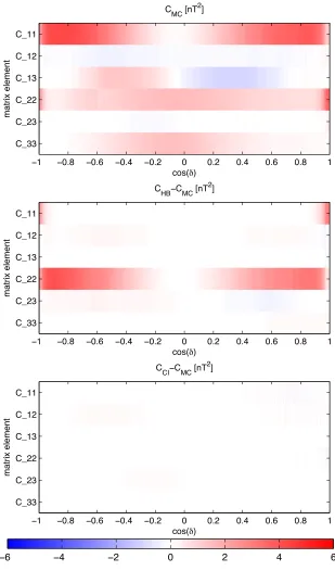
of the 3217 CHAMP rotation cases on the horizontal axis, but sorted by their cosδ value. Recall from Eq. (44) that the columns of Abecome orthonormal whenδ = π/2 or cosδ = 0. The six matrix elements are in the order of the first column, followed by the bottom two elements of the second column, followed by the lower-right corner ele-ment. The middle panel is the same except that the matrix is nowCHB−CMC, and the last panel is also the same except the matrix is now CCI −CMC. The scales are equivalent in all three panels. Clearly there is a high level of agree-ment betweenCCIandCMCfor all rotation cases, but much less agreement betweenCHBandCMC, except in the vicin-ity of cosδ =0. While agreement would be expected near cosδ = 0 in the isotropic case, it is not clear that agree-ment would occur in the anisotropic case (σ2
χ =σδ2 =σλ2),
even thoughAhas orthonormal columns. The maximum absolute deviation from CMC is 5.77 nT2 for CHB and it occurs in element (2,2)when cosδ = 0.99359. ForCCI this number is 0.35 nT2and it also occurs in element(2,2) when cosδ = −0.99953. Figure 1 shows that many of the CHB−CMCvalues are often larger than the corresponding values ofCMC, particularly in the(2,2)elements (matrix el-ement 4 on the vertical axis of Fig. 1). While the use ofCHB has proven beneficial in magnetic field modeling to date, the use ofCCIcould be a significant improvement, especially as models attempt to describe finer details of Earth’s magnetic field.
5.
Development of the Advanced CI Algorithm
An advanced CI algorithm will now be built upon the foundation outlined in Section 2 with improvements from SIVW in Section 3 and the revised treatment of vector mag-netometer attitude errors in Section 4. The modified param-eterization will be described as well as howSwarm gradi-ent information is to be exploited for improved lithospheric recovery which entails a more sophisticated error analysis then was used in the basic algorithm.5.1 Parameterization
The parameterization for the advanced algorithm is listed in Table 2 and is similar to the basic algorithm in the core field except for higher time resolving splines that are higher in order and knot density. The lithosphere is now split into two parameter types, “nominal” and “nuisance”, that will be discussed in the next section. The magnetosphere is the same as in the basic algorithm while the ionosphere is dif-ferent in that itsa prioriconductivity model now has 3D structure (Kuvshinov, 2011). If(ω)andιιι(ω)are the vec-tors of SH coefficients for the inducing and induced iono-spheric fields, respectively, at frequencyω, then thea priori
coupling via the conductivity model is manifested in the re-lationshipιιι(ω) = Q(ω)(ω), where Q(ω) is the coupling matrix at frequencyω. In a 1D treatment, as in Sabakaet al
(2002, 2004) and Sabaka and Olsen (2006),Q(ω)is diago-nal and square and its elements are only dependent upon SH degree. In the full 3D treatment,Q(ω)is a dense, generally rectangular matrix allowing for very complicated induced structure to result from relatively smooth inducing struc-ture. Therefore, the change from 1D to 3D comes from sim-ply using a different set ofQ(ω). In addition, toroidal mag-netic fields due to meridional currents that exist within the
satellite sampling shells are also modeled in the advanced CI algorithm. These follow the parameterization of CM4 (Sabakaet al., 2004). Finally, because OHM data are now processed in the advanced algorithm, static vector biases are now included in the parameter set for each observatory in order to absorb effects such as local crustal anomalies (Sabakaet al., 2002, 2004).
The truly new parameters are those that describe the netometer alignment, that is, the rotation of the vector mag-netometer measurementBVFMin the VFM frame to CRF
BCRF=RCRF←VFMBVFM. (48)
For Swarm, this rotation is parameterized by a set of 3 positive counter-clockwise Euler angles of type(X Y Z)for each satellite such that (Olsenet al., 2013)
RCRF←VFM=Rˆz(γ )Rˆy(β)Rˆx(α),
= ⎛
⎝cossinγγ −cossinγγ 00 0 0 1
⎞ ⎠
⎛
⎝ cos0β 0 sin1 0β
−sinβ 0 cosβ
⎞ ⎠
× ⎛
⎝10 cos0α−sin0 α 0 sinα cosα
⎞
⎠. (49)
In the advanced CI algorithm the observation equations in-volving vector magnetometer measurements are expressed in the CRF. If the model parameter vector at thek-th GN stepxk is split into two subsets, the “geophysical”
param-eters in vectorzk and the Euler parameters for a particular
satellite in vectorek, then for thei-th vector measurement BVFMi of that satellite, the observation equation is
0= −RCRF←VFM(ek)BVFMi +gi(zk)+ηηηi, (50)
=ai(xk)+ηηηi, (51)
whereηηηi is the error vector, andgi(zk)andai(xk)are the
geophysical and total model vectors in the CRF, respec-tively. The reason for solving in the CRF rather than the VFM frame is to decouple the productRTCRF←VFMgi(zk)that
exists in the latter system, thus decreasing the level of non-linearity in the estimation process. Recalling Eq. (6), it can be seen that Eq. (51) is in a form that is equivalent to having di =0.
Note that while the magnetospheric and associated in-duced field parameters described so far are estimated by iteratively solving LSLE-GN in Eq. (6) using Eqs. (7) and (8), they do not represent the final Level-2 product MMA SHA 2because they are only estimated during geo-magnetic quiet times. Rather, they provide a crucial step in the generation of these products, which is elaborated upon further in Section 7.5. This is the reason for using the term “precursor” in Table 2.
5.2 ExploitingSwarmgradient information
One of the great advantages of theSwarmconstellation is that the low satellite pair have orbits that differ only by 1.4◦in the values of their Right Ascension of the Ascend-ing Node (RAAN), thus allowAscend-ing for east-west gradiome-try to be carried out at low-mid latitudes. Let theSwarm
Fig. 1. Comparison of attitude error covariances (in nT2) computed with different methods over 3217 instances of CHAMP rotations from inertial frame
J2000 to the CHAMP CRF. Top panel shows covariance computed via Monte Carlo simulation of sizeN =1000, second panel shows difference between Monte Carlo covariance and that computed from the HB theory, and last panel shows difference between Monte Carlo covariance and that computed from the CI method. Vertical axes are the six independent elements of the covariance matrices, specifically the first column followed by the last two elements of the second column followed by the lower-right corner element. The horizontal axis shows the 3217 instances of rotation sorted by cosδ.
(r, θ, φ+φ), respectively, wherer,θ, andφare the ra-dius, colatitude and longitude, respectively, andφ is a longitude increment. Assume that they provide vector mea-surementsBECEF(r, θ, φ)andBECEF(r, θ, φ+φ)that have been rotated into the Earth Centered Earth Fixed (ECEF) frame, where thezaxis points to the north geographic pole, thex axis points along the prime meridian, and the yaxis completes the right-handed system. If these vectors are
fur-ther rotated into the local spherical NEC frame at the mid-point of the satellite positions, then for smallφ certain components of their difference behave as a negative gradi-ent of a potgradi-ential function whose SH coefficigradi-ents are multi-plied by a gain factor of approximately
G−(m)=
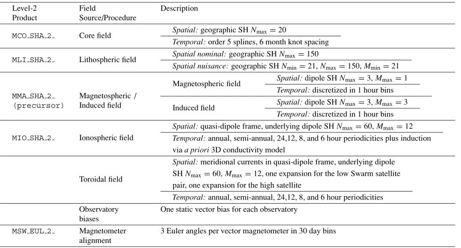
Table 2. The advanced CI source parameterization and corresponding Level-2 product label.
MCO SHA 2 Core field Spatial:geographic SHNmax=20
Temporal:order 5 splines, 6 month knot spacing
MLI SHA 2 Lithospheric field Spatial nominal:geographic SHNmax=150
Spatial nuisance:geographic SHNmin=21,Nmax=150,Mmin=21
MMA SHA 2 (precursor)
Magnetospheric / Induced field
Magnetospheric field Spatial:dipole SHNmax=3,Mmax=1
Temporal:discretized in 1 hour bins Induced field Spatial:dipole SHNmax=3,Mmax=3
Temporal:discretized in 1 hour bins
MIO SHA 2 Ionospheric field
Spatial:quasi-dipole frame, underlying dipole SHNmax=60,Mmax=12
Temporal:annual, semi-annual, 24,12, 8, and 6 hour periodicities plus induction viaa priori3D conductivity model
Toroidal field
Spatial:meridional currents in quasi-dipole frame, underlying dipole SHNmax=60,Mmax=12, one expansion for the low Swarm satellite pair, one expansion for the high satellite
Temporal:annual, semi-annual, 24,12, 8, and 6 hour periodicities Observatory
biases
One static vector bias for each observatory
MSW EUL 2 Magnetometer alignment
3 Euler angles per vector magnetometer in 30 day bins
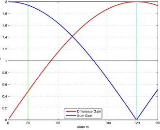
as compared to the potential coefficients leading to the indi-vidual field measurements. These components correspond to the direction of the ECEFzaxis in the NEC frame and the direction of the average of the two measurement vectors in the NEC frame. If these two directions are coincident, then all components will exhibit this gain enhancement. It can be seen that 0≤ G−(m)≤ 2 and that within the range 0 ≤ m ≤ 150, the maximum gain for vector difference measurements is found at approximatelym = 129. Con-versely, certain components of their sum behave as a nega-tive gradient of a potential function whose SH coefficients are multiplied by a gain factor of approximately
G+(m)=
2+2 cosmφ. (53)
These components correspond to the direction of the ECEF
zaxis in the NEC frame and the direction of the difference of the two measurement vectors in the NEC frame. Again, if these two directions are coincident, then all components will exhibit this gain. Note that these gain factors are out of
phase such that
G2
−(m)+G+2(m) = 2. The gain factors
are shown in Fig. 2 for the order range of the core and crustal fields and are derived in Appendix B.
If one were only interested in recovering high de-gree/order lithospheric signals, then based on the gain fac-tors one might naively exclude the vector summation data and focus only on the vector differences. However, the sum-mation data is critical for determining broad-scale, highly time varying fields such as the magnetospheric and the high-frequency induced fields, which if not properly modeled can cause spurious signals that mimic lithospheric signal. This strongly suggests using the SIVW mechanism in order to preserve the vector summation data, but account for sys-tematic bias in its high degree/order lithospheric signal that must certainly exist, especially given its low gain factors at high orders. Because the CRFs ofSwarmA and B (CRFA
and CRFB, respectively) cannot be considered the same, the CI algorithm first rotates the observation equations for each satellite to the local NEC coordinate system at the mid-point between the two satellites before adding and subtracting. If RMP←CRFA andRMP←CRFB be the rotations from CRFAand CRFB to the mid-point, respectively, then a given pair of vector measurements fromSwarmA and B are transformed to differences and sums via the following orthogonal trans-formation
The covariances are similarly transformed as
At this point, the observation equations and covariance of Eqs. (54) and (55) could be formally introduced into the LSLE-GN framework of Eq. (6), with the modification of an additional infinite variance term in the covariance to ac-count for high degree/order lithospheric systematic bias in the vector summations. In practice, however, it is much more feasible to perform this through co-estimation of nui-sance parameters as shown in Section 3. This means that while Eq. (6) is strictly followed, Eqs. (7) and (8) are modi-fied to include the crustal nuisance parameters. This essen-tially modifies theAkmatrix in the previous equations and
Fig. 2. Plot of the gain factors versus SH ordermfor potential field SH coefficients when simple differences (red) and summations (blue) of vector measurements of theSwarmlow pair are used. The horizontal black line indicates a gain of unity. The vertical green line atm=20 delineates the region above where summation data is considered too contaminated for inclusion in the nominal crustal field model. The vertical cyan line indicates the order of maximum gain for difference data, which is approximatelym=129.
be
⎛ ⎜ ⎜ ⎝
d−
d+
dC
dOHM
⎞ ⎟ ⎟
⎠=
⎛ ⎜ ⎜ ⎝
Ar
− Ah− 0
Ar
+ Ah+Ah+
ArC AhC AhC ArOHM 0 0
⎞ ⎟ ⎟ ⎠
⎛ ⎝xxrh
nh
⎞
⎠, (56)
where the subscript “k” has been suppressed, the subscripts “−”, “+”, “C”, and “OHM” indicate vector differences, summations,Swarmsatellite C (the high satellite), and the ground observatories, respectively, and the superscripts “h” and “r” indicate the high degree/order lithospheric field pa-rameters containing systematic bias in the summation data, and the remainder of the parameters, respectively. Like-wise,xh,nh, andxrare the vector adjustments to the nominal and nuisance high degree/order lithospheric fields, and the remaining nominal parameters, respectively. Note that because of its high altitude, the measurements from
SwarmC are assumed to have a low SNR in the high de-gree/order lithospheric field, and are therefore eliminated from the nominal model. In the case of the OHM mea-surements, the static vector biases that are solved for effec-tively decouple this data from the static lithosphere and so it is not affected by either the nominal or nuisance litho-spheric parameters, at least for n > 20. The C matrix in Eqs. (7) and (8) is now that in Eq. (55). However, in the current implementation of the CI algorithm,C−+is ig-nored. Again, it should be stated that when solving LSLE-GN, only the nominal parameters are used to calculatedk
and Ak and are the only parameters updated. The
nui-sance parameters are only included to expedite the use of the dense SIVW covariance matrix. In this study, the high
degree/order lithospheric nuisance field is defined to be in the rangen,m>20, as shown by the green vertical line in Fig. 2, and so does not include the time varying part of the internal field.
5.3 Weighting and robust estimation
The next task is to define C in Eqs. (7) and (8) for each measurement type. For the vector differences and summations, this is commensurate to defining CAA and CBB in Eq. (55). Beginning with the simplest case, the OHM measurement noise covariance is expressed in the form COHM = σOHM2 I, where σOHM2 is a function of ge-omagnetic latitude with polar stations having higher vari-ance than lower latitude stations. Thus the noise is treated as isotropic and uncorrelated between vector components and other data. Likewise, satellite scalar measurements are treated as uncorrelated with all other data and the variance is denoted by σ2
F. For satellite vector measurements, the
formalism of Section 4 is employed to account for the CRF attitude error while an additional isotropic term is added to account for instrument noise (Holme, 2000) and is cho-sen here to match the scalar variance, which is assumed the same for each spacecraft fluxgate magnetometer. Therefore, CAA=σF2I+CCRFA(xk)andCBB=σF2I+CCRFB(xk).
No-tice that because the attitude error (second term) is a func-tion of BCRF(xk), thenCAA andCBB change at each GN iteration. Specifically, bothCCRFA(xk)andCCRFB(xk)are in
the form of Eq. (35) under the assumptions of Section 4.3. These vector measurements are also assumed uncorrelated with all other data.
the2norm of a vector, as does LSLE-GN, would provide the maximum-likelihood estimate. Since this is rarely the case in real-world problems, the estimator can suffer delete-rious effects due to excessive influence of outliers. To com-bat this, a robust estimation procedure know as “Iteratively Reweighted Least-Squares” (IRLS) with Huber weighting will be employed here (Constable, 1988). This method has been used successfully in such models as CM4 (Sabakaet al., 2004) where details may be found. What is important here is that the IRLS formulation is defined for uncorre-lated, scalar measurements. IRLS assigns Huber weights to thei-th measurement at thek-th GN iteration as a function of its standard deviationσi and current residualei,k
accord-ing to
where the underlying Huber distribution is defined as hav-ing a Gaussian core for |ei,k| ≤ cσi, and Laplacian tails
(Constable, 1988). A value ofc=1.5 is used by the CI al-gorithm. All measurement types conform to the structure of Eq. (57) except the vector differences and summations. To rectify this, the Huber weighting is applied to the principle components of the covariance in Eq. (55), which follows readily from the eigendecompositions ofCAAandCBB.
In Appendix A it is shown thatEuu=0. It follows from
Eq. (35) thatCCRFABCRFA = 0, which means that CCRFA exists in a 2-dimensional subspace that is spanned by the columns of a 3×2 matrixU⊥Athat are orthogonal toBCRFA. The eigendecomposition ofCAAis then given by
CAA=
whereBˆCRFA is the unit vector in the direction of BCRFA, UCRFA =U⊥AUAis a 3×2 matrix whose columns span the range of CCRFA, and UAAUTAis the eigendecomposition ofUT⊥ACCRFAU⊥Awhere the 2×2 matrixUAis orthogonal and the 2×2 matrixA is diagonal with positive eigen-value entries. Of course a similar development leading to Eq. (58) applies toCBB. Thus, using Eq. (55) and Eq. (58) the residuals are rotated into the principle axes of the covari-ance matrix in Eq. (55) whereσ2
F,σF2I+AandσF2I+B supply theσi needed for determining the Huber weighting
in Eq. (57).
5.4 Regularization
What remains is to define the quadratic norms in Eq. (8) that are used to regularize the system. For the core SV and ionosphere the norms are similar to those used in the CM4 model (Sabakaet al., 2004) and earlierSwarm sim-ulation studies (Sabaka and Olsen, 2006). A combination of the mean-squared magnitude ofB¨rover the sphere at the core-mantle boundary (CMB) and at Earth’s surface were used to constrain the core SV, while the nightside iono-spheric E-region currents were minimized by including a norm that measures the mean-squared magnitude of the E-region equivalent current, Jeq, flowing at 110 km over the night-time sector defined as 1100–0500 hrs local time. In
addition, these currents are further smoothed by minimiz-ing the mean-squared magnitude of the surface divergence of the diurnally varying portion ofJeqat mid-latitudes at all local times.
For this study two additional norms were employed. The first is motivated by the presence of a gap in the coverage of the satellites resulting in a polar cap of a few degrees in half-angle. Because zonal SH terms are most affected by these gaps, a norm which minimizes the square of the magnetic potential of the lithospheric field for degreesn≥60 at both the north and south geographic poles was developed. The final norm minimizes the sum of square deviations of the Euler angles in each time bin with the average value over the entire mission domain as determined from the current nominal values. This is done separately for each of the three angles.
In summary, Nq = 6 quadratic norms are applied in
Eq. (8), four of which are similar to those used in previous studies, and two of which are experimental. It is expected that similar norms will be used for the actual mission anal-ysis, but development is continuing on the CI algorithm and could quite possibly lead to better regularization techniques. The advanced CI algorithm has now been developed and will next be applied to the V2 simulation in Section 6.
6.
The V2 Simulation
The V2 closed-loop simulation is one of several levels of synthetic mission data required by ESA to validate the algo-rithms of the Level-2 data facility. This simulation uses syn-thetic data (“Test Data Set-1” or TDS-1) described in Olsen
et al.(2013) for testing the various chains of SCARF. For testing the CI chain, a data subset was used representative of geomagnetic quiet times during a 4.5 year period from July 1998 through December 2002. These quiet periods are defined as times when the geomagnetic activity index
Kp≤ 2o and the Dst-index, measuring the strength of the magnetospheric ring-current, does not change by more than 2 nT/hr. The data sampling period was set to 30 secs. The test data set contains contributions from the core field and secular variation (SV), lithospheric field, and primary and secondary ionospheric and magnetospheric fields. Note that toroidal fields where omitted from the synthetic data. Not only wasSwarmsatellite constellation data synthesized, but also a complementary OHM data set. In addition, random noise has been added to the satellite data. The requirements for the accuracy of the estimated models with respect to the reference models are listed in Table 3. The “target” and “threshold” requirements refer to desired and manda-tory levels of accuracy, respectively, based upon modeling experience.
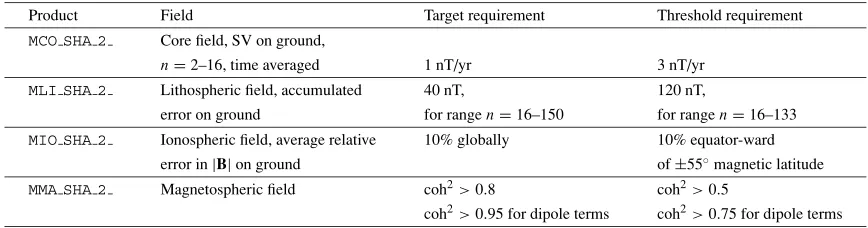
Table 3. Target and threshold requirements of estimated field accuracy for V2.
Product Field Target requirement Threshold requirement
MCO SHA 2 Core field, SV on ground,
n=2–16, time averaged 1 nT/yr 3 nT/yr
MLI SHA 2 Lithospheric field, accumulated 40 nT, 120 nT,
error on ground for rangen=16–150 for rangen=16–133
MIO SHA 2 Ionospheric field, average relative 10% globally 10% equator-ward
error in|B|on ground of±55◦magnetic latitude
MMA SHA 2 Magnetospheric field coh2>0.8 coh2>0.5
coh2>0.95 for dipole terms coh2>0.75 for dipole terms
Table 4. Angles defining rotations between VFM and CRF systems in TDS-1.
α β γ
[arcsecs] [arcsecs] [arcsecs]
Swarm A −1724 3488 −618
Swarm B 808 −434 −1234
Swarm C 2222 2991 3115
model MF7 (Maus, 2010a), and degreesn = 91–250 are taken from model NGDC-720 (version 3p1) (Maus, 2010b) scaled by factor 1.1. The primary ionospheric field is based on that of CM4 (Sabakaet al., 2004), and the secondary field SH coefficient vectorιιι(ω)is computed from the pri-mary vector(ω)at each frequencyωvia the relationship
ιιι(ω)=Q(ω)(ω)as discussed in Section 5.1. The coupling
matricesQ(ω)come from a 3D mantle conductivity model (Kuvshinov, 2011). The magnetospheric primary field is similar to that of the E2E+ simulation (Tøffner-Clausenet al., 2010) and is based on an hour-by-hour spherical har-monic analysis of worldwide distributed observatory data. The secondary magnetospheric field is computed from the same set of coupling matrices as the ionospheric field.
For synthetic satellite data, the VFM systems have been rotated with respect to their CRFs via RCRF←VFM from Eq. (49) by the amounts shown in Table 4. Note, how-ever, that TDS-1 does not include attitude error in the rotation RCRF←J2000. Their synthetic instrument noise is based upon CHAMP experience and Swarm specifica-tions and is correlated in time, but uncorrelated among vector components. More details are given in Olsen et al. (2013). The standard deviations of the noise are
(0.07,0.1,0.07) nT for (Br,Bθ,Bφ), in agreement with
Swarm performance requirements. For synthetic OHMs, isotropic noise has been applied such that the standard de-viations are(7,7,7)nT and(15,15,15)nT for locations equator-ward and pole-ward of±50◦geomagnetic latitude, respectively, for(Br,Bθ,Bφ). For the CI analysis, the
at-titude error was treated as isotropic and uncorrelated such thatCa = σa2Iin Eq. (35), whereσa = 10 arcsecs, even
though no attitude error technically exists in the TDS-1 data. The standard deviation of the isotropic instrument noise was set toσF = 3 nT, which is much larger than
present in the TDS-1 data. Although no noise has been added to the TDS-1 OHM synthetic data, the noise treat-ment in the CI follows what is actually expected from real
data, that is,C=σ2
OHMI, whereσOHM =7 and 15 nT for station locations equator-ward and pole-ward of±50◦ geo-magnetic latitude, respectively.
7.
Results and Discussion
The results of applying the advanced CI algorithm to the TDS-1 data set of the V2 simulation will now be briefly discussed. While these were found to be quite favorable, it should be stressed that this is a simulation based upon syn-thetic data containing contributions from forward models similar to those used in the CI, such as the ionospheric pri-mary and secondary fields. Therefore, it is possible that per-formance could be degraded when analyzing data from the actual mission. The three metrics employed by Sabaka and Olsen (2006) will be used here, which are defined in terms of the real and imaginary parts of complex SH coefficients of a field, denoted generically asgnmandh
m
n, respectively. 7.1 Metrics
The first metric is the Lowes-Mauersberger spectrum,
Rn(r), of Lowes (1966)
wherea andr are the reference and evaluation radii, re-spectively. TheRn(r)are the mean-square magnitude of an
internal field over a sphere of radiusr. The second metric is the degree correlation,ρn, of two fields given by
ρn=
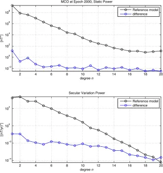
Fig. 3. TheRnspectrum of the MCO core field static part (top) and its first time derivative (bottom), or SV, at epoch 2000.0 at Earth’s surface. The black lines are the reference field and the blue lines are the difference between reference and recovered fields.
the percentage degree-normalized error in a recovered co-efficient of degreenand orderm.
There is one additional metric that will be used to eval-uate the V2 results. This is the “squared-magnitude coher-ence”, or coh2, whose range is 0 ≤ coh2 ≤ 1 and mea-sures the similarity between input and output signals of a system. For constant parameter linear systems, coh2 = 1, but this can decrease due to a number of issues, particularly the presence of noise in the system. This has been used by Olsen (1998) to analyze C-responses describing electrical conductivity of the mantle beneath Europe, and details may be found therein.
7.2 MCO core field
The Rn spectra of the MCO reference field (black) and
difference between reference and recovered fields (blue) at epoch 2000.0 at Earth’s surface are shown in the top panel of Fig. 3. The blue line falls several orders of magnitude below the black line and indicates excellent agreement be-tween the two models near the center of the model domain. The same lines are shown for SV in the bottom panel where the blue line is below the black until degreen >19. The accumulated error in SV is found to be less than 0.2 nT/yr for all times within model domain for degree n = 2–20, and thus, easily meets both the threshold and target values specified in Table 3.
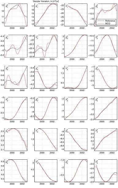
To aid in the comparison, the first time derivatives of the MCO Gauss coefficients for degreesn =1–4 are shown in Fig. 4 for the reference (black) and recovered (red) fields. The fields agree very well with most of the variations in the lines exhibited over small ranges. In fact, a comparison of the actual Gauss coefficients shows them to be almost indis-cernible over the range of coefficient values. The advanced CI algorithm is evidently recovering the MCO core field and SV to within specifications.
7.3 MLI lithospheric field
In addition to assessing the CI algorithm performance with respect to V2 accuracy requirements, it was of inter-est to see the direct benefits of taking explicit advantage of the magnetic gradient information for determination of the small-scale lithospheric field. Therefore, two types of models were derived from exactly the same magnetic field observations. The first model, denoted as “field only”, was constructed by considered theSwarmdata from three single satellites, whereas the second model, denoted as “field plus gradient”, was constructed by explicit use of the constella-tion aspect ofSwarmby using magnetic gradient informa-tion with SIVW.
The Rn spectra of the MLI reference field (black) and
Fig. 4. First time derivative, or SV, of MCO core field Gauss coefficients through time forn=1–4. The black lines are the reference field and the red lines are the recovered field.
(blue) at Earth’s surface are shown in the left panel of Fig. 5. The plots indicate a roughly two-fold reduction in power in the error per degree above aboutn = 45 when difference data are exploited. The right panel indicates a far superior
recovery of coefficients in the case of “field plus gradient” (blue) over the “field only” case (red) with regards to phase of the models, i.e., degree correlationρn. The former case
Fig. 5. Left panel isRnspectrum of reference MLI lithospheric field (black) and difference between it and a “field only” derived model (red) and between it and the final “field plus gradient” derived model (blue) at Earth’s surface. Right panel is degree correlationρnof “field only” (red) and “field plus gradient” (blue) coefficients with the reference model coefficients. The vertical dashed lines indicaten=133, which is the upper degree limit for threshold accuracy requirements.
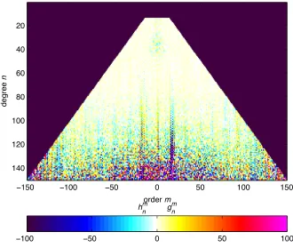
Fig. 7. MLI lithospheric field difference maps in theBr component (nT) at ground between the reference model and the “field plus gradient” derived model.
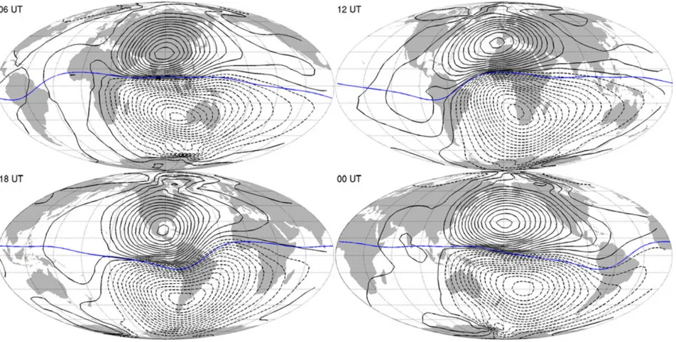
Fig. 8. Global maps of MIO ionospheric E-region equivalent current functions at vernal equinox at different universal times (UT) as recovered by the CI algorithm. Each map is centered on noon magnetic local time. The current functions exist in a sheet at 110 km altitude. Current flows in a counter-clockwise (clockwise) direction in the northern (southern) hemisphere with a 10 kA current flowing between each contour. The dip equator is shown in blue.
the true field at the 0.93 level forn=150, the degree limit of the synthetic signal. The accumulated error at ground for degreesn = 16–150 is only about 12 nT, which again is well below both the target and threshold target values for V2 accuracy.
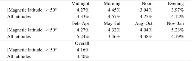
Table 5. Average relative error in|B|on ground in MIO primary ionospheric field recovery.
Midnight Morning Noon Evening
|Magnetic latitude|<50◦ 4.27% 4.45% 3.94% 3.97%
All latitudes 4.33% 4.57% 4.25% 4.12%
Feb–Apr May–Jul Aug–Oct Nov–Jan
|Magnetic latitude|<50◦ 4.27% 4.32% 4.04% 5.23%
All latitudes 5.24% 3.46% 4.38% 4.19%
Overall
|Magnetic latitude|<50◦ 4.16%
All latitudes 4.40%
approach (though not shown) for them≤20 regime, which recall, conforms to the structure of lithospheric bias treat-ment used in SIVW. There is also some improvetreat-ment in the purely sectorial terms (left and right edges).
Finally, a physical sense of the quality of the MLI litho-spheric field recovery can be seen in difference maps ofBr
at ground between the reference and “field plus gradient” models in Fig. 7. Most differences are just a few nT, ex-cept in regions around the geographic poles where they are several tens of nT. This is no doubt due to polar gaps in the
Swarmorbital coverage.
While these results suggest an optimistic outlook that the Swarmconstellation is capable of accurately recover-ing small-scale lithospheric structure, the application to real data will be more challenging, especially at high latitudes. However, if V2 performance is any indication of real perfor-mance, thenSwarmwill go far in closing the gap in inter-mediate lithospheric wavelength coverage that exists now between satellites and aeromagnetic surveys.
7.4 MIO ionospheric field
The accuracy target requirement for the MIO primary ionospheric field is 10% average relative error in |B| on ground. Table 5 actually subdivides these numbers across local time sectors (midnight, morning, noon, and evening) and across seasons (February to April, May to July, August to October, and November to January) for magnetic lati-tudes equator-ward of±50◦and all latitudes. It can be seen that every subdivision is performing almost twice as well as the 10% requirement, with overall errors of 4.16% and 4.40% for the low latitude and all latitudes regions, respec-tively.
The primary MIO ionospheric field source is modeled as an equivalent sheet current at 110 km altitude in the CI al-gorithm (Sabakaet al., 2002, 2004) and its corresponding current function has been generated from the ionospheric coefficients recovered from the V2 test and shown for dif-ferent universal times (UT) at vernal equinox in Fig. 8. This is also in very good agreement with the current function of the MIO reference field. The advanced CI algorithm ap-pears to be performing satisfactorily for this field source as well.
7.5 MMA magnetospheric/induced fields
Recall that the test data are selected for magnetically quiet times such that the CI products for core, lithosphere, and ionosphere (primary and secondary) all reflect this. However, the determination of continuous time series of the spherical harmonic expansion coefficients of magneto-spheric and corresponding induced sources requires data
taken during all geomagnetic conditions, as required for Level-2 productMMA SHA 2. Therefore, this is achieved by applying a second processing step, theMMA SHA 2 analy-sis step, after CI in the following way: Predictions are made from the output CI core, lithospheric, and primary and sec-ondary ionospheric models derived during quiet times and subtracted from each 1 minSwarmsatellite measurement and OHMs from all available ground observatories. The resulting residuals (observations minus model values) are expected to contain the magnetospheric (primary and sec-ondary) field plus errors due to improper removal of all other sources. From those residuals of each day estimates are made of the spherical harmonic expansion coefficients
qm n,s
m
n describing the external (magnetospheric) sources for Nmax =3 and Mmax =1, and coefficientsgnm,hmn
describ-ing the induced field for Nmax = Mmax = 5. This is done in bins of 1.5 hrs for the axial dipole coefficientsg0
1 andq10 (which means that 16 values for each of those coefficient pairs are determined per day) and in bins of 6 hrs for the remaining 42 coefficients (resulting in 4×42=168 values per day). In total, 200 coefficients are estimated for each day using IRLS with Huber weights.
Figure 9 shows squared-magnitude coherence (coh2) be-tween the input and the estimated time series for exter-nal (red) and induced (blue) coefficients corresponding to
Nmax =3 and Mmax =1. There is generally excellent co-herency for the external coefficients (coh2well above 0.95) and good coherence (coh2 > 0.8) for the induced coeffi-cients, in particular for periods shorter than one month or so. When using the coefficients for determination of mantle conductivity, periods up to one month correspond to resolv-ing conductivity down to 1200 km or so. P¨uthe and Ku-vshinov (2013a, b) describe the estimation of mantle con-ductivity from the Level-2 productMMA SHA 2determined in this way. Although this is a comparison between the ref-erence magnetospheric and induced fields and the output of theMMA SHA 2analysis step, it still indicates that good separation must exist between the magntospheric and in-duced fields and the others in the CI estimation. As for the accuracy requirements, the external field recovery exceeds the target values for all periods while the internal field re-covery generally exceeds the target for periods shorter than one month and are mostly above the threshold requirement for other periods.
8.
Conclusions
de-Fig. 9. Squared-magnitude coherence (coh2) between MMA reference and primary magnetospheric (red) and secondary induced (blue) Gauss coefficients determined in theMMA SHA 2analysis step following the CI algorithm.
scribed in Sabaka and Olsen (2006), and most important among these are the introduction of the SIVW mecha-nism for mitigating systematic, non-zero mean bias in the observations allowing for optimal combinations of data to achieve improved models. In addition, this paper has pointed out a way to improve on the handling of attitude er-ror in vector magnetometer data put forth in the HB theory. This will hopefully allow for even better error characteriza-tion, and thus, model quality.
The performance of the advanced CI algorithm was eval-uated using a synthetic test data set (TDS-1) from a full mission simulation. In general, it was found to perform well above both threshold and target accuracy requirements for core, lithospheric, ionospheric, and magnetospheric and in-duced. Only the recovery of induced fields at some periods longer than one month were of suspect quality. This may be due to the point-wise orthogonality condition with respect to the core field that has been imposed on this field, which of course would affect the longer periods since SV is on the order of these longer periods. Although there were no toroidal field contributions in the TDS-1 data, these fields were nonetheless co-estimated and found to be negligible, thus indicating a proper treatment in the model. All of this suggests, at least from the standpoint of V2, that the ad-vanced CI algorithm will be quite competent in delivering high quality Level-2 products.
Although the advanced algorithm is a great improve-ment over the basic algorithm, certain issues should still be dealt with to further enhance performance. Recall that when using the covariance matrix describing the error in the vector differences and summations in Eq. (55) the
cross-covariance matricesC−+have been ignored. This was done to simplify the algorithm during development, but should now be instated. The increase in deviations between ref-erence and recovered Br from the lithosphere around the
geographic poles in Fig. 7 indicates that the polar gap prob-lem should be further addressed. In addition, several issues surrounding SIVW should be explored, such as the optimal SH orderm that delineates between the nominal and nui-sance lithospheric fields, which could easily lead to better models. In addition, SIVW could be used to account for dayside bias when modeling the lithosphere, which would reflect the current best methods for crustal field modeling (Thomson and Lesur, 2007; Mauset al., 2007, 2008; Lesur
et al., 2008, 2013; Olsenet al., 2011). Finally, SIVW could be applied to high degree SV modeling by mitigating the bias due to the poor distribution of ground observatories. It is planned to implement and test several of these ideas.
Acknowledgments. We thank Richard Holme and Vincent Lesur for fruitful reviews. The NASA Center for Climate Simulation at Goddard Space Flight Center provided computer support. Some figures were produced with GMT (Wessel and Smith, 1991).