R E S E A R C H
Open Access
Retrieving the relative kernel dataset
from big sensory data for continuous queries
in IoT systems
Tongxin Zhu
1, Jinbao Wang
1*, Siyao Cheng
1, Yingshu Li
2and Jianzhong Li
1Abstract
Internet of Things (IoT) is rapidly developed and widely deployed in recent years, which makes the sensory data generated by IoT systems explode. The huge amount of sensory data generated by some IoT systems has already exceeded the storage, transmission, and computation capacities of IoT systems. However, the valuable sensory data which is highly related to a query in an IoT system is relatively small. The sensory data which is highly related to a queryQforms the relative kernel dataset ofQ. Therefore, retrieving sensory data in the relative kernel dataset of a query instead of the raw sensory data will reduce the heavy burdens of an IoT system in terms of transmission and computation and then reduce the energy consumption of the IoT system. In this paper, we investigate the problem of retrieving relative kernel dataset from big sensory data for continuous queries in IoT systems. Two algorithms, relative kernel dataset retrieving algorithm and piecewise linear fitting-based relative kernel dataset retrieving algorithm, are proposed to retrieve the relative kernel dataset for continuous queries. Beside, algorithms for estimating the answers of continuous queries based on their relative kernel datasets are also proposed. Extensive simulation results are provided to verify the effectiveness and energy efficiency of the proposed algorithms.
Keywords: Internet of things, Big sensory data, Relative kernel dataset
1 Introduction
The Internet of Things (IoT) system, which refers to the network with a variety of intelligent things or objects around us, provides an efficient way to observe the com-plicated physical world and brings convenience to our life. With the repaid development of wireless telecommunica-tions, embedded systems, and sensing techniques, the IoT systems are widely developed and generate mass sensory data. Gartner forecasts that there will be 20.8 billion con-nected things by 2020 and 100 billion by 2030 [1]. Such a large scale of IoT systems will generate mass sensory data. According to [2], the global climate data will reach to 100 petabytes in 2020. Other types of sensory data, such as monitoring data from a large-scale system (e.g., Large Hadron Collider) and GPS data, also increase rapidly and have exceeded terabytes or even petabytes currently.
*Correspondence:[email protected]
1School of Computer Science and Tech, Harbin Institute of Technology, Harbin, China
Full list of author information is available at the end of the article
The mass sensory data generated by IoT systems is called as big sensory data, which has four V characters.
• Volume. The volume of big sensory data is extremely huge that has already exceeded the storage,
transmission and computation capacities of IoT systems.
• Variety. An IoT system always contains a wide variety of sensors to satisfy the complex applications of the IoT system.
• Velocity. To improve the accuracy of applications in an IoT system, the sampling frequency of each sensor is high. Therefore, the generating velocity of big sensory data is quite fast.
• Value. The value of big sensory data always concentrates on a relative small subset of the big sensory data on account of the existence of noises and redundancies in big sensory data.
The Volume, Variety, and Velocity characters of big sensory data make the data processing in IoT systems
more challenging. The mass sensory data may exceed the storage, transmission and computation capacities of IoT systems. Besides, the energy consumption for trans-mitting and computing big sensory data is quite high. Therefore, the existing sensory data acquisition, rout-ing [3–6], data collection [7–9], and data computation [10, 11] techniques are no longer applicable for the big sensory data. The authors in [3] design cluster-based rout-ing protocol for wireless sensor networks with nonuni-form distribution of sensors. The works of [4–6] focus on constructing connected dominating sets for wire-less sensor networks. However, the transmission of mass sensory data will exceed the communication capacity of wireless sensor networks and affect the effectiveness of these methods accordingly. The authors in [7] study the approximated holistic aggregation algorithms based on uniform sampling. And the authors in [8] propose aggregation scheduling algorithms for energy harvest-ing sensor networks. However, the mass sensory data will increase the aggregation latency and affect the per-formances of these algorithms. The work of [9] pro-poses algorithm to track quantiles and range countings in wireless sensor networks. The authors in [10] pro-pose algorithm to support curve query processing in wireless sensor networks. The work in [11] studies the application-aware scheduling in wireless networks. When the amount of sensory data is huge, the computation com-plexity of these algorithms may exceed the computation capability of wireless sensor networks. Therefore, a series of new in-network processing algorithms with much lighter transmission and computation overloads should be considered.
TheValuecharacter of big sensory data reveals that the dataset of sensory data that is highly related to a given query is usually small. Therefore, for a query, only retriev-ing the dataset of sensory data that is highly related to the query will greatly reduce the transmission and computa-tion overhead of an IoT system and then reduce the energy consumption of the IoT system.
There already exists some data reduction algorithms which reduce the amount of sensory data transmitted and computed in an IoT system and then reduce the energy consumption of the IoT system. Firstly, the simplest data reduction technique is based on sampling [12–16]. How-ever, the sampling technique is only applicable to some simple statistic queries. Some valuable data in other types of queries may be missed by sampling technique on account of the limitation of sampling frequency. Besides, the sampled data may not be necessary for all queries. Secondly, another classical technique for in-network data reduction is compressed sensing [17–22]. However, com-pressed sensing only considers the temporal and spatial correlation between sensory data while neglecting the correlation between the queries conducted by users and
the sensory data generated by different sensors. As a consequence, the data reduction for a given query is not enough in compressed sensing. Thirdly, the work proposed by Cheng et. al. is the first one to investigate data processing problem in big sensory data [23, 24]. The work can reduce sensory data by drawing domi-nant dataset from Big Sensory Data. Nevertheless, the dominant dataset defined in [23,24] is irrelevant to any given query. As with the sampling technique and com-pressed sensing technique, the sensory data in the domi-nant dataset defined in [23,24] may not be necessary for all queries.
All existing algorithms above are not energy efficient enough since they ignore the correlation between a given query and the sensory data. As a consequence, we concen-trate on retrieving the relative kernel dataset for continu-ous queries from big sensory data in IoT systems in this paper. The relative kernel dataset of a query is the sensory data that is highly related to the query. The amount of sen-sory data in the relative kernel dataset of a query is usually small according to theValuecharacter of big sensory data. Therefore, only transmitting and computing these sen-sory data will highly reduce the energy consumption of an IoT system. Besides, many applications in the IoT systems provide users to have access to temporal variation infor-mation of the monitored environment. That is, users can conduct continuous queries in IoT systems to monitor the physical world in real time, where a continuous query is a query which is conducted by a user continuously and fre-quently. Since continuous queries are frequent in an IoT system, reducing the energy consumption of continuous queries will highly reduce the energy consumption of an IoT system.
On account of the above reasons, we study the problem of retrieving the relative kernel dataset from big sen-sory data for continuous queries in IoT systems in this paper. Two algorithms, the relative kernel dataset retriev-ing (RKDR) algorithm and the piecewise linear fittretriev-ing- fitting-based relative kernel dataset retrieving (PLF-RKDR) algo-rithm, are proposed firstly to retrieve the relative kernel dataset for continuous queries. Besides, two algorithms, the piecewise linear fitting-based answer estimating (PLF-AE) algorithm and temporal correlation-based answer estimating (TC-AE) algorithm, are proposed to estimate the answers of continuous queries based on their relative kernel datasets. The major contributions of this paper are as follows.
1 The definition of the relative kernel dataset of a continuous query is proposed firstly. Besides, the relative kernel dataset retrieving problem is formally defined in this paper.
relative kernel dataset from big sensory data for continuous queries in IoT systems.
3 Two algorithms, the PLF-AE algorithm and the TC-AE algorithm, are proposed to estimate the answers of continuous queries in an IoT system based on their relative kernel datasets.
4 Extensive simulations on both simulation dataset and real dataset are carried out to verify the accuracy of the proposed algorithms.
The rest of this paper is organized as follows. Section2 summarizes the methods of this paper. Section3presents the problem definition. Section 4 elaborates the algo-rithms for the relative kernel dataset retrieving prob-lem. Section5provides the algorithms for estimating the answers of continuous queries with their relative kernel datasets. Section6analyzes the performances of the pro-posed algorithms. Section7shows the simulation results and discussion. Section 8 discusses the related work. Finally, Section9concludes the whole paper.
2 Methods
In this paper, we study the problem of retrieving the rel-ative kernel dataset from big sensory data for continuous queries in IoT systems. The Pearson correlation coeffi-cient is applied to measure the linear correlation between sensory data and the continuous queries. Besides, the piecewise linear fitting method is applied to approximate the relationships between sensory data and the continu-ous queries. Two algorithms are proposed to retrieve the relative kernel dataset for continuous queries in IoT sys-tems. Another two algorithms are proposed to estimate the answers of continuous queries with their relative ker-nel datasets. The absolute error and relative error are defined and evaluated on both simulation dataset and real dataset. The simulation results show that the proposed algorithms are effective and efficient.
3 Problem definition 3.1 The IoT system model
An IoT system is equipped with n categories of sen-sors, which can generate n types of sensory data from the monitored environment. Each type of sensory data is described as an attribute of the monitored environ-ment. The attribute set of the monitored environment is denoted asA = {x1,x2,· · ·,xn}. For each continuous
queryQ from users at time slottin an IoT system, the IoT system returns an answer to users according to the sensory data collected at time slott. The answer of query
Qis described as the target value of queryQ, denoted as
yq. Apparently, the target valueyqis correlated with
par-tial or allnattributes. Taking the healthcare monitoring IoT system as an example, there are a variety of sensors collecting data of heart sounds, electrical heart signals,
blood oxygen saturation, respiratory sounds, blood pres-sure, body temperature, etc., which are attributes of this IoT system. When the user’s query is the possibility of car-diac arrest, the IoT system returns a probability. In this application, the queryQis the possibility of cardiac arrest and the target valueyqis the returned probability.
3.2 The correlation model
To explore the correlations between attributes inAand queryQ, a training set withmtraining examples is applied. Each training example is denoted as a column vectorSl=
[x1l,· · ·,xnl,yql]T, whereT denotes the matrix transpose
andxil(1≤i≤n) is the value of attributexiandyqlis the
target value of queryQin training exampleSl, 1≤l≤m.
The training set can be denoted as a(n+1)×mmatrix
S=[S1,S2,· · ·,Sm].
In most applications of IoT systems, the sensory data can reflect the statement of the monitored physical world intuitively. That means the simple linear correlation can reveal the relationship between the sensory data and the query of an IoT system in most cases. The Pearson cor-relation coefficient is a common metric to measure the linear correlation between two variables in correlation analysis. The value of the Pearson correlation coefficient is in [−1, 1], where−1 presents the total negative linear correlation, 0 presents no linear correlation, and 1 is the total positive linear correlation. Therefore, we apply the Pearson correlation coefficient to measure the correlation between attributes and the correlation between attributes and continuous queries.
Firstly, the Pearson correlation coefficient of any two attributesxi andxj(1 ≤ i ≤ n, 1 ≤ j ≤ nandi = j) is
presented by the following formula,
rij=
m
l=1(xil−xi)(xjl−xj)
m
l=1(xil−xi)2ml=1(xjl−xj)2
(1)
where xil is the value of attribute xi andxjl is the value
of attribute xj in training example Sl. Besides, xi = 1
m
m
l=1xil is the average value of attribute xi andxj = 1
m
m
l=1xjlis the average value of attributexjin the
train-ing setS.
Secondly, the Pearson correlation coefficient of attribute
xi (1 ≤ i ≤ n) and the target valueyq of a continuous
queryQis presented by the following formula,
Rqi =
m
l=1(xil−xi)(yql−yq)
m
l=1(xil−xi)2ml=1(yql−yq)2
(2)
wherexildenotes the value of attributexiandyqldenotes
the target value of queryQin training exampleSl. Besides,
yq = m1 ml=1yql is the average value of target values of
3.3 Problem statement
In this paper, we study the problem of retrieving the rela-tive kernel dataset for continuous queries in IoT systems to reduce the transmission and computation overhead and energy consumption of the IoT systems. The formal def-inition of the relative kernel datasetKqfor a continuous queryQis described as follows.
Definition 1(β-compatible) Given a parameter β, where 0 < β < 1, any two attributes xi and xj are β-compatible if their Pearson correlation coefficient rij satisfies that |rij| ≤ β, where rij is calculated by formula (1).
Definition 2(β-compatible set) Given a parameterβ, where0 < β <1, the subsetASof attribute setAis aβ -compatible set if any two attributes inASareβ-compatible with each other, i.e.,AS⊆Aand∀xi,xj∈AS,|rij| ≤β.
Definition 3(the weight of a β-compatible set) Given
a β-compatible set AS and a continuous query Q, the
weight ofASis denoted as w(AS). The definition of w(AS) is w(AS) = xi∈AS|R
q
i|, where R q
i is the correlation coefficient between attribute xiand query Q.
Definition 4((k,β)-relative kernel dataset Kq) Given the attribute setA, query Q, the compatible parameterβ, and the required size k of the relative kernel dataset, a training setS. The(k,β)-relative kernel dataset of query Q is a subset ofA, denoted asKq, satisfying the following three conditions.
(1)Kqis aβ-compatible subset, (2) the size ofKqis at most k, and
(3) w(Kq) >w(AS)for any attribute subsetASsatisfying conditions (1)(2).
Based on the definition of(k,β)-relative kernel dataset
Kq, we define the problem of retrieving the relative
kernel dataset for continuous queries in IoT systems as follows.
Problem statement The problem of retrieving the rela-tive kernel dataset for continuous queries in IoT systems is denoted as relative kernel dataset retrieving (RKDR) problem. The input and output of the RKDR problem are presented as follows.
Input:
1. The attribute set of an IoT system,
A= {x1,x2,· · ·,xn}; 2. The continuous query,Q ;
3. The training set,S =[S1,S2,· · ·,Sm];
4. The required size of the relative kernel dataset,k ; 5. The compatible parameter,β.
Output:
The(k,β)-relative kernel datasetKqof the continuous queryQ;
Theorem 1The RKDR problem is NP-hard.
Proof 1 The Maximum Weighted Budgeted Indepen-dent Set (MWBIS) problem is to find a maximum weighted independent set in a weighted graph G(V,E)of cardinal-ity at most k. The MWBIS problem has been proved to be NP-hard in [25]. The MWBIS problem can be converted to the RKDR problem in polynomial time. Each vertex i of the weighted graph G(V,E)can be regarded as an attribute xi of an IoT system, where the weight of vertex i can be regarded as the absolute value of the correlation coefficient between attribute xi and query Q. For each edge(i,j) ∈E in the weighted graph G(V,E), we regard that attributes xi and xjare notβ-compatible. To find a maximum weighted independent set of cardinality at most k is to find the
(k,β)-relative kernel dataset of query Q. Then the MWBIS problem is converted to the RKDR problem. Therefore, the RKDR problem is NP-hard.
4 Algorithms for the relative kernel dataset retrieving problem
In this section, we propose two algorithms to retrieve the relative kernel dataset for continuous queries in IoT systems, which are the relative kernel dataset retrieving (RKDR) algorithm and the piecewise linear fitting-based relative kernel dataset retrieving (PLF-RKDR) algorithm. The detailed description of the RKDR algorithm is pre-sented in Algorithm 1 and the detailed description of the PLF-RKDR algorithm is presented in Algorithm 3. The RKDR algorithm is suitable for the IoT systems where sim-ple linear correlation can reveal the relationship between the sensory data and the continuous queries. And the PLF-RKDR algorithm is more suitable for the IoT sys-tems where the correlation between an attribute and a continuous query is not merely linear correlation.
4.1 Relative kernel dataset retrieving algorithm
The relative kernel dataset retrieving (RKDR) algorithm firstly reduces redundancies in attributes by measuring the linear correlations between different attributes. Then, the Pearson correlation coefficient is applied to mea-sure the correlations between attributes and the given continuous query. The RKDR algorithm contains the fol-lowing two steps.
Step 1. Calculate the candidate relative kernel dataset through reducing the redundancies in attributes.
The candidate relative kernel dataset is denoted asX. At first, the candidate relative kernel dataset is initialized as the attribute set, i.e.,X =A= {x1,· · ·,xn}. Then,Xis
Step 1.1. For each attributexi(1≤i≤n)inX, the
Pear-son correlation coefficient Rqi betweenxi and the target
valueyqof queryQis calculated by formula (2).
Step 1.2 For any two attributexiandxjinX, the Pearson
correlation coefficientrijof them is calculated by formula
(1). Ifxiandxjare notβ-compatible (i.e.,|rij| > β), one
of them is redundant inX and should be removed. Ifxi
has stronger linear correlation with queryQthanxj, i.e.,
|Rqi| > |Rjq|, remove xj from X. Otherwise, remove xi
fromX.
After the above two sub-steps, the candidate relative kernel dataset X is calculated through reducing redun-dancies in attributes.
Step 2. Retrieve the(k,β)-relative kernel dataset from the candidate relative kernel dataset.
Any two attributes in the candidate relative kernel dataset X are β-compatible according to Step 1.2. The Pearson correlation coefficient of each attribute inX and query Q is calculated in Step 1.1. The absolute values of these Pearson correlation coefficients are calculated. Therefore, we select the top-k absolute values of these Pearson correlation coefficients and their correspondingk
attributes. The top-kabsolute values of these Pearson cor-relation coefficients are denoted as|Rqa1| ≥ |R
q
a2| ≥ · · · ≥
|Rqak|and the correspondingkattributes arexa1,· · ·,xak. Thesekattributes are added to the(k,β)-relative kernel dataset of queryQ, i.e.,Kq= {xa1,· · ·,xak}.
After the above two steps, the (k,β)-relative kernel dataset for query Q is derived. The detailed operations are formally described in Algorithm 1. Algorithm 1 is proposed to retrieve the(k,β)-relative kernel dataset for
Algorithm 1:Relative Kernel Dataset Retrieving Algo-rithm
Input: queryQ, the attribute setA, the training set
S =[S1,· · ·,Sm], the compatible parameterβ, the
10 Otherwise, removexifromX;
11 Obtain the top-kcorrelations, denoted by{|Rqa1|,· · ·,|R
q ak|};
12 Kq= {xa1,· · ·,xak};
13 ReturnKq.
continuous queryQin IoT systems by the linear correla-tion analysis.
4.2 Piecewise linear fitting-based relative kernel dataset retrieving algorithm
In some scenarios, linear correlation is not enough to describe the relationship between an attribute and a con-tinuous query. For example, the correlation between an attribute and a continuous query could be exponential, quadric, or logarithmic. In this situation, the RKDR algo-rithm proposed in the last subsection may be no longer applicable. As a consequence, the piecewise linear fitting-based relative kernel dataset retrieving (PLF-RKDR) algo-rithm is proposed to improve the RKDR algoalgo-rithm in this subsection.
Since it is almost impossible to know the actual cor-relation function between an attribute and a continuous query, it is difficult to measure the correlation coeffi-cient between them. The PLF-RKDR algorithm applies the piecewise linear fitting method to approximate the actual correlation function between an attribute and a contin-uous query. Since each segment of the piecewise linear function is a linear function, the PLF-RKDR algorithm combines the Pearson correlation coefficients of all seg-ments in the piecewise linear function to measure the correlation of each attribute and the continuous query. The PLF-RKDR algorithm contains the following three steps.
Step 1. Calculate the Pearson correlation coefficient of each attribute xi ∈ A and the continuous query Qby
piecewise linear fitting.
We apply the training setS to calculate the piecewise linear function between each attribute xi ∈ A and the
target value of the continuous queryQ.
Firstly, for each training example Sl (1 ≤ l ≤ m), we extract the tuple (xil,yql), where xil is the
value of attribute xi and yql is the target value in Sl. Then, we sort the extracted tuples by the
non-descending order of the values of attribute xi and
denote the ordered tuples as {(x1i,y1q),· · ·,(xmi ,ymq)}, wherex1i ≤ · · · ≤xmi .
Secondly, the optimal segment points of the sorted tuples {(x1i,y1
q),· · ·,(xmi ,ymq)} are calculated recursively
by the method proposed in [26]. For one segment, {(xsi,ysq),(xsi+1,yqs+1),· · ·,(xei,yeq)}, the linear fitting func-tion of it is derived by the least-squares method and is denoted as Fi(s,e)(x). The error sum of squares of lin-ear fitting function Fi(s,e)(x) is E(s,e). The optimal seg-ment point (xji,yjq) of {(xsi,ysq),(xis+1,ysq+1),· · ·,(xei,yeq)}
should satisfy that j = arg mins<l<e(E(s,l) + E(l,e)).
This process is conducted recursively until E(s,e) −
Algorithm 2: Least-Squares Based Piecewise Linear Fitting (LS-PLF) Algorithm
Input: Two endpointssande,E(s,e), the thresholdγ Output: The set of segment pointsP
1 ife−s>1then divided into li − 1 subsets according to the calculated
segment point set Pi. Each subset is denoted as Dj =
{(xsij,ysqj),· · ·,(xsij+1,y sj+1
q )}, wheresj,sj+1 ∈ Pi, and 1 ≤ j<li. The Pearson correlation coefficientRqijfor subsetDj
is calculated by the following formula,
Rqij=
As a consequence, the correlation coefficient of attribute
xiand the continuous queryQis the weighted average of
the absolute values of all calculated Pearson correlation coefficients {Rqij|1 ≤ j < li}, which is presented as the
Step 2. Calculate the candidate relative kernel datasetX through reducing the redundancies in attributes.
Initially, all attributes are added toX, i.e.,X = A = {x1,· · ·,xn}. Then, for each two attributexi,xj ∈ X, we
compute the Pearson correlation coefficientrijof them by
formula (1). When|rij| > β, meaning that xi andxj are
notβ-compatible,xi andxj are redundant inX and one
of them should be removed.|Rqi|and|Rqj|are compared, whereRqi andRqj are calculated by formula (4). If|Rqi| >
|Rqj|, removexjfromX. Otherwise,xiis removed fromX.
Step 3. Retrieve the relative kernel dataset from the can-didate relative kernel dataset for the continuous query
Q.
After Step 2, all attributes in candidate relative kernel datasetX areβ-compatible. Then, we can obtain the
top-kcorrelation coefficients of all attributes inX calculated in Step 1 and the corresponding kattributes. The top-k
correlation coefficients are denoted asRqa1 ≥R
q
a2 ≥ · · · ≥
Rqak, and the corresponding k attributes are denoted as
xa1,xa2,· · ·,xak. Finally, the(k,β)-relative kernel dataset of queryQisKq= {xa1,xa2,· · ·,xak}.
After the above three steps, the (k,β)-relative kernel dataset of queryQis calculated. The detailed operations are formally described in Algorithm 3. Algorithm 3 is proposed to retrieve the (k,β)-relative kernel dataset of continuous queryQin IoT systems by the piecewise linear fitting method. And Algorithm 2 is called by Algorithm 3 to return the set of segment points for piecewise linear fitting.
Algorithm 3:PLF-Relative Kernel Dataset Retrieving Algorithm
Input: queryQ, the attribute setA, the training set
S=[S1,· · ·,Sm], the compatible parameterβ, the required sizek, thresholdγ
Output:(k,β)-relative kernel datasetKq 1 X =A= {x1,x2,· · ·,xn};
2 foreach attribute xiinXdo
3 Extract the tuples(xil,yql)from training exampleSl (1≤l≤m);
4 Sort the extracted tuples by non-descending order of the values of attributexi, i.e.,{(x1i,y1q),· · ·,(xmi ,ymq)}, 8 Calculate the Pearson correlation coefficientRqijby
formula (3);
16 Otherwise, removexifromX;
17 Obtain the top-kcorrelations, denoted by{|Rqa1|,· · ·,|Rqak|}; 18 Kq= {xa1,· · ·,xak};
19 ReturnKq.
5 Algorithms for estimating the answer of a continuous query with its relative kernel dataset
IoT system should return an answer of Qto the users. In this section, we propose two algorithms to estimate the answers of continuous queries with their relative ker-nel datasets, which are the piecewise linear fitting-based answer estimating (PLF-AE) algorithm and the temporal correlation-based answer estimating (TC-AE) algorithm. The detailed descriptions of the PLF-AE algorithm and the TC-AE algorithm are presented in Algorithm 4 and Algorithm 5, respectively. The PLF-AE algorithm is pro-posed to estimate the answers for continuous queries with their (k,β)-relative kernel datasets by piecewise lin-ear fitting method. And the TC-AE algorithm is proposed to estimate the answers for continuous queries with less energy consumption by applying the temporal correla-tions of sensor data.
5.1 Piecewise linear fitting-based answer estimating algorithm
The piecewise linear fitting-based answer estimating (PLF-AE) algorithm applies the piecewise linear fitting method to estimate the answer of a continuous query with sensory data of attributes in its (k,β)-relative kernel dataset. Once a continuous queryQis issued by users in an IoT system at time slott, only sensory data of attributes in the (k,β)-relative kernel datasetKqofQare transmit-ted to the sink node. For each attribute, the sensory data generated at time slottis denoted asxi(t). That is, the sink
node collects sensory data in{xi(t)|xi ∈ Kq}to estimate
the answer ofQ. Firstly, the piecewise linear function of each attribute inKqand the target value of queryQis
cal-culated by the piecewise linear fitting method. Then, each piecewise linear function is assigned a weight. Finally, the target value ofQat time slottis estimated by the sensory data of attributes inKqaccording to the weighted piece-wise linear functions. The PLF-AE algorithm consists of the following three steps.
Step 1. Calculate the piecewise linear functions of query
Qand attributes inKq.
For each attributexi ∈ Kq, the piecewise linear
func-tion of xi and queryQ is denoted asfi. The process of
calculatingficonsists of the following three sub-steps.
Step 1.1. Preprocess the training setS = {S1,· · ·,Sm}.
For each training exampleSl (1 ≤ l ≤ m), the value
of attributexi and the target valueyql are extracted and
denoted as a tuple(xil,yql). All extracted tuples are sorted by the non-descending order of the values of attributexi.
The sorted tuples are denoted as{(x1i,y1
q),· · ·,(xmi ,ymq)},
wherex1i ≤ · · · ≤xmi .
Step 1.2. Calculate the optimal segment points of piece-wise linear functionfi.
The optimal segment points offiis calculated by
Algo-rithm 2. The returned segment point set is denoted as
Pi = {s1,s2,· · ·,sli}. As a consequence, the sorted tuples
{(x1i,y1
q),· · ·,(xmi ,ymq)} are divided into li − 1 subsets,
where each subsetDj (1 ≤ j < li ) is denoted as Dj =
{(xsij,ysqj),· · ·,(xsij+1,ysqj+1)}.
Step 1.3. Calculate the linear functions for all subsets. For each subset Dj = {(xisj,ysqj),· · ·,(xsij+1,ysqj+1)}, the
linear function is calculated by the least-squares method and is denoted asfi,j. The Pearson correlation coefficient Rqijfor subsetDjis calculated by formula (3). As a
conse-quence, the piecewise linear functionfiof attributexiand
the continuous queryQis as follows.
fi=
Step 2. Assign weights for the calculated piecewise lin-ear functions.
For each attributexi∈Kq, the generated sensory data at
time slottisxi(t). Ifxi(t)satisfies thatxisj <xi(t)≤ xsij+1
(sj,sj+1∈Piand 1≤j<li), the piecewise linear function fi is assigned a weight with wi = |Rqij|, where R
q ij is the
Pearson correlation coefficient calculated in Step 1. Step 3. Estimate the target value of queryQat time slot
t.
Based on the sensory data generated at time slott, i.e., {xi(t)|xi∈Kq}, the estimated target value ofQat time slot tis calculated by the following formula.
The detailed operations for the PLF-AE algorithm is described in Algorithm 4. Algorithm 4 is proposed to estimate the answers of continuous queries with their (k,β)-relative kernel datasets by piecewise linear fitting method.
5.2 Temporal correlation-based answer estimating algorithm
It has been revealed by many research works that the monitored physical environment always varies continu-ously [27, 28]. That means the difference between the sensory data of an attribute in two continuous time slots may be small. Consequently, the temporal correlation-based answer estimating (TC-AE) algorithm utilizes the temporal correlation between sensory data of an attribute to estimate the answer of a continuous query with less energy consumption.
In the PLF-AE algorithm, each time a continuous query
Algorithm 4: Piecewise Linear Fitting Based Answer Estimating Algorithm
Input: the training setS=[S1,· · ·,Sm],(k,β)-relative kernel datasetKqof queryQ, the sensory data collected at time slott,{xi(t)|xi∈Kq} 1 .Output: the estimated answeryq(t)
2 foreach attribute xiinKqdo
3 Extract the tuples(xil,yql)from training exampleSl (1≤l≤m);
4 Sort the extracted tuples by non-descending order of the values of attributexi, i.e.,{(x1i,y1q),· · ·,(xmi ,ymq)}, 8 Calculate the Pearson correlation coefficientRqijby
formula (3);
9 Calculate piecewise linear functionfi,jby the least-squares method;
10 The piecewise linear functionfiis calculated by formula (5);
The sink node of an IoT system stores the latest received sensory data of all attributes, denoted as{b1,b1,· · ·,bn}.
Besides, for each attributexi ∈A, the corresponding
sen-sor also stores its latest transmitted sensen-sory data bi. For
each attributexi∈A, there exists a value range [pi,qi] for
its sensory data,i.e.,∀t,pi ≤xi(t) ≤qi. When a
continu-ous queryQis conducted by users, only sensory data in a subset of{xi(t)|xi ∈Kq}are transmitted to the sink node.
For each attributexi∈Kq,xi(t)is transmitted to the sink
node only ifxi(t)satisfies that|xi(t)−bi| ≥α×(qi−pi),
where 0 ≤ α ≤ 1 is a user-defined adjustable constant. Applying this method, the energy consumption of the IoT system can be further reduced with a little sacrifice of the accuracy for estimating the answer of a continuous query. Through adjustingα, we can balance the tradeoff between the energy consumption and the estimation accuracy.
If the sensory data xi(t) satisfies that |xi(t) − bi| ≥
α×(qi−pi), the stored sensory data in the
correspond-ing sensor is updated tobi =xi(t). Besides, after the sink
node receivedxi(t), it also updates its stored sensory data
to bi = xi(t). After the sink node has received all
sen-sory data{xi(t)|xi ∈ Kq,|xi(t)−bi| ≥α×(qi−pi)}, the
sink node estimates the answer ofQby the similar method described in the PLF-AE algorithm.
The detailed operations for the TC-AE algorithm is described in Algorithm 5. Algorithm 5 is proposed to
Algorithm 5: Temporal Correlation Based Answer Estimating Algorithm
Input: the training setS=[S1,· · ·,Sm],(k,β)-relative kernel datasetKqof queryQ, the stored sensory data{bi|xi∈A}, the parameterα, the sensory data
6 Sort the extracted tuples by non-descending order of the values of attributexi, i.e.,{(x1i,y1q),· · ·,(xmi ,ymq)}, 10 Calculate the Pearson correlation coefficientRqijby
formula (3);
11 Calculate piecewise linear functionfi,jby the least-squares method;
12 The piecewise linear functionfiis calculated by formula (5);
estimate the answers of continuous queries with their (k,β)-relative kernel datasets by piecewise linear fitting method. Algorithm 5 can further reduce the sensory data transmitted and computed in an IoT system by applying the temporal correlations of sensory data.
6 The performance analysis
6.1 Computation complexity of the RKDR algorithm The computation complexity of computing the Pearson correlation coefficients between queryQandnattributes isO(mn). Then, the computation complexity of calculat-ing the Pearson correlation coefficients between any two attributes is O(mn2). Therefore, the computation
com-plexity of Step 1 isO(mn2). The computation complexity
of sorting nPearson correlation coefficients in Step 2 is
O(nlogn). In conclusion, the computation complexity for
the RKDR algorithm isO(mn2).
O(nmlogm). Then, the computation complexity of calcu-lating optimal segment points fornattributes isO(nm3). Finally, the computation complexity of calculating the cor-relation coefficients between query Q and attributes is
O(nm). Therefore, the computation complexity of Step 1 isO(nm3). The computation complexity of calculating candidate relative kernel dataset in Step 2 isO(mn2). In Step 3, the computation complexity of sorting all correla-tion coefficients isO(nlogn). In conclusion, the
computa-tion complexity for the PLF-RKDR algorithm isO(nm3).
6.3 Computation complexity of the PLF-AE algorithm and the TC-AE algorithm
The computation complexity of the PLF-AE algorithm and the computation complexity of the TC-AE algo-rithm are similar. For each attribute xi ∈ Kq, the
following computations are conducted. Firstly, the com-putation complexity of sorting the extracted tuples {(x1i,y1q),· · ·,(xmi ,ymq)} isO(mlogm). Then, the compu-tation complexity of calculating optimal segment points isO(m3). Finally, the computation complexity of calcu-lating the Pearson correlation coefficients and piecewise linear functions for all segments isO(m). Therefore, the computation complexity of the algorithm isO(km3).
7 Simulation results and discussion
In this section, the performances of the RKDR algo-rithm and the PLF-RKDR algoalgo-rithm are evaluated by extensive simulations on both simulation dataset and real dataset. The RKDR algorithm and the PLF-RKDR algo-rithm retrieve the(k,β)-relative kernel datasets for con-tinuous queries. The application of the RKDR algorithm and the PLF-RKDR algorithm is to estimate the answers of the continuous queries given by users in IoT systems with the retrieved(k,β)-relative kernel datasets. There-fore, to evaluate the performances of the RKDR algorithm and the PLF-RKDR algorithm, we evaluate the accuracy of the answers estimated by the retrieved(k,β)-relative kernel datasets of continuous queries. The PLF-AE algo-rithm and the TC-AE algoalgo-rithm are proposed in this paper to estimate the answers of continuous queries by the retrieved(k,β)-relative kernel datasets.
The simulation dataset consists of two sub-datasets, which are about two functionsyq = f1(x1,· · ·,x15) and
yq = f2(x1,· · ·,x15), respectively. There are 15 attributes of the IoT systems, which arex1,x2,· · ·,x15. There are two continuous queries of the IoT systems, which are query
Q1and queryQ2. Each training example in the simulation dataset includes the values of 15 attributes and the tar-get values of queryQ1and queryQ2following functionf1 andf2, respectively. We apply the RKDR algorithm and the PLF-RKDR algorithm to retrieve the(k,β)-relative kernel dataset for queryQ1 and query Q2. Then, we apply the PLF-AE algorithm and the TC-AE algorithm to estimate
the target values of query Q1 and query Q2 with the retrieved(k,β)-relative kernel dataset.
The real dataset is collected from a mobile device. The collected data from the mobile device contains 6 attributes, i.e. the X-, Y-, and Z-axes of a three-axis accelerometer and theX-,Y-, andZ-axes of a three-axis gyroscope of the mobile phone, and a motion type of a person holding the mobile phone. Each training exam-ple is generated by a person holding the mobile device and making 7 types of motions, which are numbered as motion 1 to 7. Each training example contains values of 6 attributes and a target valueyqindicating which type of
motion happens. We apply the RKDR algorithm and the PLF-RKDR algorithm to retrieve the (k,β)-relative ker-nel dataset for the motion query, where the(k,β)-relative kernel dataset is a subset of 6 attributes of the mobile phone. Then, we apply the PLF-AE algorithm and the TC-AE algorithm to estimate the motion type of the person holding the mobile phone with the retrieved(k,β)-relative kernel dataset.
In the following simulations, two types of error are applied to evaluate the performance of the proposed algorithms. The first one is the absolute error er1 = |yq(t)−yq(t)
yq(t) |, whereyq(t) is the target value estimated by sensory data of attributes in the (k,β)-relative kernel datasetKqretrieved by the proposed algorithms andyq(t)
is the true target value of queryQ at time slott. How-ever, the true target value of queryQis always unknown or inaccessible in the monitored physical world. As a con-sequence, another type of error replaces yq(t) by yq(t),
whereyq(t)is the target value estimated by sensory data of allnattributes. The second type of error is called as the
relative error, denoted aser= |yq(t)−y
q(t)
yq(t) |.
In the following subsections, the comparison experi-ments are firstly conducted to compare the performances of the RKDR algorithm and the PLF-RKDR algorithm. Then, both absolute error and relative error are evaluated on simulation dataset to verify the performance of the proposed algorithms. Finally, experiments on real dataset are carried out to verify the performance of the proposed algorithms.
7.1 Comparison experiments of the RKDR algorithm and the PLF-RKDR algorithm
We compare the RKDR algorithm and the PLF-RKDR algorithm by conducting a group of comparison exper-iments on simulation dataset. We compare the relative error er = |yq(t)−yq(t)
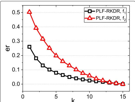
Fig. 1The relative error of RKDR algorithm and PLF-RKDR algorithm on the simulation dataset
In Fig.1, the relative error of both algorithms decreases whenkincreases. However, the relative error of the PLF-RKDR algorithm is much smaller than that of the PLF-RKDR algorithm no matter how muchkis. In particular, the rel-ative error of the PLF-RKDR algorithm is almost a half of the RKDR algorithm whenkis larger than 5. Therefore, the PLF-RKDR algorithm has better performance than the RKDR algorithm. Besides, Fig. 1 shows that the relative error of both algorithms on simulation dataset with func-tionf1is much less than that of functionf2, which reveals that linear correlation cannot describe the relationship between sensory data and queryQ2perfectly.
7.2 The performance of proposed algorithms on simulation dataset
7.2.1 The absolute error on simulation dataset
The first group of simulations is conducted on the simula-tion dataset to evaluate the performance of the PLF-RKDR algorithm through the absolute error. Firstly, the PLF-RKDR algorithm is applied to retrieve the(k,β)-relative kernel datasets of continuous queries. Then, the PLF-AE algorithm is applied to estimate answers of continu-ous queries. Finally, the absolute error of the estimated answers of the continuous queries are evaluated. The simulation results are presented in Figs.2and3.
Firstly, we investigate the impact of k, the size of the (k,β)-relative kernel dataset, on the absolute error of the estimated answers of the continuous queries. Figure 2 presents the absolute error under three test sets, whose size are T = 1000,T = 500, andT = 100. The data points presented in Fig. 2 are the average of simulation results on 1000, 500, and 100 times of query, respectively. Figure2 presents that the absolute error decreases with the increasing ofk. It is shown that the absolute error can
Fig. 2The impact ofkon the absolute error of PLF-RKDR algorithm on the simulation dataset
reach to 0.258 whenkis only 5, which is pretty small for users.
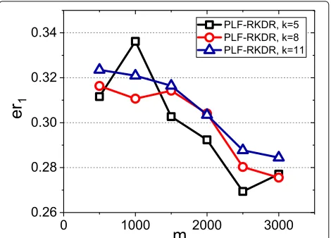
Then, we study the impact ofm, the size of training set, on the absolute error of estimated answers of the continu-ous queries. Figure3presents the absolute error when the size of the(k,β)-relative kernel dataset arek =5,k =8, andk=11. Each data point presented in Fig.3is the aver-age of simulation results on 500 times of query. Figure3 reveals that the absolute error of estimated answers of the continuous queries decreases sharply with the increasing ofm.
7.2.2 The relative error on simulation dataset
The second group of simulations is carried out on the sim-ulation dataset to evaluate performance of the PLF-RKDR algorithm. Firstly, the PLF-RKDR algorithm is applied on the simulation dataset to retrieve the (k,β)-relative
kernel datasets of queryQ1and queryQ2. Then, the PLF-AE algorithm is applied to estimate answers of query
Q1 and query Q2. Finally, the relative error of the esti-mated answers of query Q1 and queryQ2 is evaluated. The simulation results are presented in Figs.4and5. Each data point presented in Figs. 4 and 5 is the average of simulation results on 500 times of query.
Firstly, we investigate the impact ofk, the size of the (k,β)-relative kernel dataset, on the relative error of the estimated answers of query Q1 and queryQ2. The size of training set is set asm = 3000. When the size of the (k,β)-relative kernel dataset is fixed, the relative error of the estimated answers of queryQ1and queryQ2are dif-ferent since difdif-ferent queries have difdif-ferent relative kernel datasets. That explains why we need to retrieve the rel-ative kernel dataset for each given query. Figure4shows that the relative error of the estimated answers of both queries decreases with the increasing ofk. Specially, Fig.4 presents that the relative error is reduced to 0.05 whenk
is only a half ofn. That means the IoT system can save a half of energy consumption when sacrificing only a few accuracy.
Then, we study the impact of m, the size of training set, on the relative error of the estimated answers of the continuous queries. In the simulations, different scales of training set are evaluated and the size of the(k,β)-relative kernel dataset is set ask = 8. We evaluate the relative error with the size of training setmvarying from 500 to 3000 with increment of 500. Figure5presents that the rel-ative error decreases slowly withm increases. Similarly, the relative error of the estimated answers of queryQ1is less than that of queryQ2. It is worth noting that evenm is only 500, the relative error is less than 0.15 whenkis no less than a half ofn.
Fig. 4The impact ofkon the relative error of PLF-RKDR algorithm on the simulation dataset
Fig. 5The impact ofmon the relative error of PLF-RKDR algorithm on the simulation dataset
7.3 The performance of the proposed algorithm on real dataset
In this subsection, simulations are conducted on the real dataset to evaluate the performance of the PLF-RKDR algorithm. Each training example of the real dataset con-sists of the values of 6 attributes and a target value indicating which type of motion happens. For each type of motion i, the target value is set as 1 if motion i
happens; otherwise, the target value is set as 0. Firstly, the (k,β)-relative kernel datasets for motion 1 to 7 are retrieved by the RKDR algorithm. Then, the PLF-AE algorithm is applied to estimate the target value of each motion, respectively. Finally, if the target value of a motioni calculated by the PLF-AE algorithm with its (k,β)-relative kernel dataset retrieved by the PLF-RKDR algorithm is larger than 0.5, it is thought that motion i
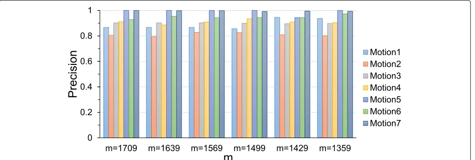
happens. To evaluate the performance of the PLF-RKDR algorithm, we evaluate the precision of the judgement of each motion. The simulation results are presented in Figs.6and7.
The first group of simulations are conducted to study the impact ofkon the motion judgement precision. The size of training set is fixed to m = 4796. The simula-tion results are presented in Fig.6, where each data point is the average of the simulation results on 1511 times of query. Figure6presents that the precision for each motion increases with k increases. The reason is similar to the analysis of simulations on the simulation dataset. For each type of motion, more than 80% of the queries are correctly answered by the PLF-RKDR algorithm and the PLF-AE algorithm.
Fig. 6The impact ofkon the precision of PLF-RKDR algorithm on the real dataset
data point presented in Fig.7is the average of simulation results on 585 times of query. Figure7presents that more than 80% of the motions are correctly judged.
8 Related works
Reducing the energy consumption of an IoT system through reducing sensory data transmitted and computed in the IoT system has been studied for a long time. The existing data reduction algorithms can be divided into two categories. The first category of algorithms are based on sampling. The second category of algorithms are based on compressed sensing.
The first category of data reduction algorithms is sampling-based data reduction algorithms. The authors in [12] investigate Bernoulli sampling-based aggrega-tion algorithms, which can satisfy arbitrary precision requirement. They firstly adapt the sampling probabil-ity to satisfy the arbitrary precision requirement given
by users. Then, the aggregation is approximately com-puted with the sampled sensory data. The work in [13] proposes a sampling-based algorithm to compute approx-imate quantiles in sensor networks. The authors apply random sampling in the algorithm and provide a guar-antee that the computed φ-quantile are within error with a constant probability which can arbitrarily close to 1. The algorithms proposed in [14] adapt the sampling frequencies for energy-hungry sensors in wireless sensor networks according to the real needs of the monitored physical environment. As a consequence, the proposed algorithms can reduce the sensory data by sampling and then reduce the energy consumption of a wireless sen-sor network. Another work in [15] adaptively adjusts the sampling frequency to retrieve the critical data points of each sensor, which can significantly reduce the energy consumption. The authors in [16] apply adaptive sam-pling in snow monitoring applications of wireless sensor networks. They proposed algorithms to dynamically esti-mate the sampling frequencies of sensors to minimize sensory data sensed and transmitted in sensor networks while maintaining acceptable accuracy of the monitoring application.
The second category of data reduction algorithms is compressed sensing-based data reduction algorithms. The authors in [17] propose an algorithm combining the compressed sensing with the principal component analysis. The algorithm can recover the whole dataset through a small subset of data, which can significantly reduce the sensory data transmitted in the network. Other two works [18, 19] are proposed to compress the sensory data in a wireless sensor network by the principal component analysis technique. The work in [20] applies the compressed sensing in both single-sink and multi-single-sink wireless sensor networks to effi-ciently gather sensory data. The authors in [21] propose
a compressed sensing-based approach to monitor with vehicular networks. The tradeoff between the communi-cation cost and the estimation accuracy is studied in this work. The authors in [22] proposed an algorithm to mini-mize the energy consumption of sensor networks through joint routing and compressed aggregation. Compressed sensing-based data reduction algorithms compress raw sensory data and transmit compressed sensory data in the network.
However, the sampling based data reduction algorithms in the first category are only effective for some simple statistic queries, such as maximum, quantile, and aver-age. These algorithms cannot reduce sensory data for arbitrary queries. Besides, the compressed sensing-based data reduction algorithms in the second category only consider the temporal and spatial correlations between sensory data but ignoring the correlation between the sensory data and the queries. The sensory data can be further reduced if the correlations between sensory data and queries of IoT system are taken into considera-tion. And the data reduction for a given query is not enough in these algorithms. Another work is proposed in [23,24] to retrieve the dominant dataset from big sensory data for a wireless sensor network. However, the domi-nant dataset defined in [23, 24] is a general one for all queries instead of a specific one for a given query. As a consequence, the existing algorithms cannot retrieve the relative kernel dataset for continuous queries in IoT systems.
9 Conclusion
This paper studies the problem of retrieving the rela-tive kernel dataset from big sensory data for continu-ous queries in IoT systems. The RKDR algorithm and PLF-RKDR algorithm are proposed to retrieve the(k,β) -relative kernel dataset for continuous queries. Besides, the PLF-AE algorithm and TC-AE algorithm are proposed to estimate the answers of continuous queries based on their (k,β)-relative kernel datasets. Extensive simulations are carried out to evaluate the performances of the proposed algorithms.
Abbreviations
IoT: Internet of Things; LS-PLF: Least-squares-based piecewise linear fitting; PLF-AE: Piecewise linear fitting-based answer estimating; PLF-RKDR: Piecewise linear fitting-based relative kernel dataset retrieving; RKDR: Relative kernel dataset retrieving; TC-AE: Temporal correlation-based answer estimating
Acknowledgements
This work is partly supported by the National Natural Science Foundation of China under Grant NO. 61632010, 61502116, U1509216, 61370217, and 61602129 and the National Science Foundation (NSF) under grant NO.1741277.
Funding
This work is partly supported by the National Natural Science Foundation of China under Grant NO. 61632010, 61502116, U1509216, 61370217 and 61602129 and the National Science Foundation (NSF) under grant NO.1741277.
Availability of data and materials
No applicable.
Authors’ contributions
TX designed the idea, performed the experiments, and wrote the manuscript. JB and SY gave valuable suggestions on the design of the study. YS assisted in processing the data and helped to finish the simulation results. JZ supervised the work and helped to check and revise the manuscript. All authors read and approved the final manuscript.
Competing interests
The authors declare that they have no competing interests.
Publisher’s Note
Springer Nature remains neutral with regard to jurisdictional claims in published maps and institutional affiliations.
Author details
1School of Computer Science and Tech, Harbin Institute of Technology, Harbin, China.2Department of Computer Science, Georgia State University, Atlanta, USA.
Received: 2 October 2018 Accepted: 3 May 2019
References
1. G. G. Says, 6.4 billion connected things will be in use in 2016, up 30 percent from 2015 (2015).http://www.gartner.com/newsroom/id/3165317
2. J. T. Overpeck, G. A. Meehl, S. Bony, D. R. Easterling, Climate data challenges in the 21st century. Science.331(6018), 700–702 (2011). American Association for the Advancement of Science
3. J. Yu, Y. Qi, G. Wang, X. Gu, A cluster-based routing protocol for wireless sensor networks with nonuniform node distribution. AEU-Int. J. Electr. Commun.66(1), 54–61 (2012). Elsevier
4. J. Yu, N. Wang, G. Wang, Constructing minimum extended
weakly-connected dominating sets for clustering in ad hoc networks. J. Parallel Distrib. Comput.72(1), 35–47 (2012). Elsevier
5. J. Yu, X. Ning, Y. Sun, S. Wang, Y. Wang, inINFOCOM 2017-IEEE Conference on Computer Communications, IEEE. Constructing a self-stabilizing cds with bounded diameter in wireless networks under sinr (IEEE, 2017), pp. 1–9 6. T. Shi, S. Cheng, Z. Cai, J. Li, inIEEE INFOCOM 2016-The 35th Annual IEEE
International Conference on Computer Communications. Adaptive connected dominating set discovering algorithm in energy-harvest sensor networks (IEEE, 2016), pp. 1–9
7. J. Li, S. Cheng, Z. Cai, J. Yu, C. Wang, Y. Li, Approximate holistic aggregation in wireless sensor networks. ACM Trans. Sens. Netw. (TOSN).
13(2), 11 (2017). ACM
8. Q. Chen, H. Gao, Z. Cai, L. Cheng, J. Li, inIEEE INFOCOM 2018-IEEE Conference on Computer Communications. Energy-collision aware data aggregation scheduling for energy harvesting sensor networks (IEEE, 2018), pp. 117–125
9. Z. He, Z. Cai, S. Cheng, X. Wang, Approximate aggregation for tracking quantiles and range countings in wireless sensor networks. Theor. Comput. Sci.607, 381–390 (2015). Elsevier
10. S. Cheng, Z. Cai, J. Li, Curve query processing in wireless sensor networks. IEEE Trans. Veh. Technol.64(11), 5198–5209 (2015)
11. X. Zheng, Z. Cai, J. Li, H. Gao, A study on application-aware scheduling in wireless networks. IEEE Trans. Mob. Comput.16(7), 1787–1801 (2017). IEEE 12. S. Cheng, J. Li, Q. Ren, L. Yu, inProceedings of the 29th Conference on
Information Communications. Bernoulli sampling based (ε,
δ)-approximate aggregation in large-scale sensor networks (IEEE Press, 2010), pp. 1181–1189
13. Z. Huang, L. Wang, K. Yi, Y. Liu, inProceedings of the 2011 ACM SIGMOD International Conference on Management of Data. Sampling based algorithms for quantile computation in sensor networks (ACM, 2011), pp. 745–756
15. T. Zhu, S. Cheng, Z. Cai, J. Li, Critical data points retrieving method for big sensory data in wireless sensor networks. EURASIP J. Wirel. Commun. Netw.2016(1), 18 (2016)
16. C. Alippi, G. Anastasi, C. Galperti, F. Mancini, M. Roveri, inMobile Adhoc and Sensor Systems, 2007. MASS 2007. IEEE International Conference On. Adaptive sampling for energy conservation in wireless sensor networks for snow monitoring applications (IEEE, 2007), pp. 1–6
17. R. Masiero, G. Quer, D. Munaretto, M. Rossi, J. Widmer, M. Zorzi, inGlobal Telecommunications Conference, 2009. GLOBECOM 2009. IEEE. Data acquisition through joint compressive sensing and principal component analysis (IEEE, 2009), pp. 1–6
18. S. V. Macua, P. Belanovic, S. Zazo, inSignal Processing Advances in Wireless Communications (SPAWC), 2010 IEEE Eleventh International Workshop On. Consensus-based distributed principal component analysis in wireless sensor networks (IEEE, 2010), pp. 1–5
19. A. Rooshenas, H. R. Rabiee, A. Movaghar, M. Y. Naderi, inIntelligent Sensors, Sensor Networks and Information Processing (ISSNIP), 2010 Sixth
International Conference On. Reducing the data transmission in wireless sensor networks using the principal component analysis (IEEE, 2010), pp. 133–138
20. H. Wang, Y. Zhu, Q. Zhang, inINFOCOM, 2013 Proceedings IEEE. Compressive sensing based monitoring with vehicular networks (IEEE, 2013), pp. 2823–2831
21. H. Zheng, S. Xiao, X. Wang, X. Tian, M. Guizani, Capacity and delay analysis for data gathering with compressive sensing in wireless sensor networks. IEEE Trans. Wirel. Commun.12(2), 917–927 (2013). IEEE
22. L. Xiang, J. Luo, A. Vasilakos, inSensor, Mesh and Ad Hoc Communications and Networks (SECON), 2011 8th Annual IEEE Communications Society Conference On. Compressed data aggregation for energy efficient wireless sensor networks (IEEE, 2011), pp. 46–54
23. S. Cheng, Z. Cai, J. Li, X. Fang, in2015 IEEE Conference on Computer Communications (INFOCOM). Drawing dominant dataset from big sensory data in wireless sensor networks (IEEE, 2015), pp. 531–539
24. S. Cheng, Z. Cai, J. Li, H. Gao, Extracting kernel dataset from big sensory data in wireless sensor networks. IEEE Trans. Knowl. Data Eng.29(4), 813–827 (2017)
25. T. Kalra, R. Mathew, S. P. Pal, V. Pandey, inConference on Algorithms and Discrete Applied Mathematics. Maximum weighted independent sets with a budget (Springer, 2017), pp. 254–266
26. T. L. L. Zong-tian, Leasts-quares method piecewise linear fitting. Comput. Sci.39(6A), 482–484 (2012)
27. S. Cheng, J. Li, Z. Cai, inINFOCOM, 2013 Proceedings IEEE. O (ε)-approximation to physical world by sensor networks (IEEE, 2013), pp. 3084–3092