Position estimation with a millimeter wave massive MIMO system based on distributed steerable phased antenna arrays

R E S E A R C H

Open Access

Position estimation with a

millimeter-wave massive MIMO system based on

distributed steerable phased antenna arrays

Nenad Vukmirovi´c

, Miloš Janji´c

, Petar M. Djuri´c

and Miljko Eri´c

Abstract

In this paper, we propose a massive MIMO (multiple-input-multiple-output) architecture with distributed steerable phased antenna subarrays for position estimation in the mmWave range. We also propose localization algorithms and a multistage/multiresolution search strategy that resolve the problem of high side lobes, which is inherent in spatially coherent localization. The proposed system is intended for use in line-of-sight indoor environments. Time

synchronization between the transmitter and the receiving system is not required, and the algorithms can also be applied to a multiuser scenario. The simulation results for the line-of-sight-only and specular multipath scenarios show that the localization error is only a small fraction of the carrier wavelength and that it can be achieved under reasonable system parameters including signal-to-noise ratios, antenna number/placement, and subarray apertures. The proposed concept has the potential of significantly improving the capacity and spectral/energy efficiency of future mmWave massive MIMO systems.

Keywords: Direct position estimation, mmWave, Massive MIMO, Steerable phased antenna arrays, Wireless indoor localization

1 Introduction

Millimeter-wave (mmWave) communication and mas-sive MIMO (multiple-input-multiple-output) are disrup-tive technologies for cellular 5G (5th generation) systems. Not surprisingly, they have been in the focus of inten-sive research efforts in both academia and industry in the last decade. The application of massive MIMO sys-tems in the mmWave band represents a big research and technological challenge. Since the work of Marzetta in 2010 [1], there have been many technical papers on this technology. Some address system issues [2–6], and others signal processing [7], analog and hybrid beamforming [8–17], propagation and channel modeling/measurement [18–20], technological aspects [21], and practical imple-mentations [22,23].

Multi-user MIMO systems referred to as massive MIMO systems were introduced in [1]. Unlike in conventional M IMO systems for point-to-point communications where the

*Correspondence:[email protected]

1_{School of Electrical Engineering, University of Belgrade, Belgrade, Serbia} Full list of author information is available at the end of the article

channels between pairs of antennas are assumed uncorre-lated, in massive MIMO systems there is a large number of antennas at a base station (BS). The antennas of the system form beams toward low-cost user devices with spatially separated single antennas [1]. Many antennas are required in the mmWave band because of the high pathloss and the need for large antenna gains to obtain sufficiently high signal-to-noise ratios (SNRs).

Traditionally, beamforming by the antennas is realized completely in the digital domain. This entails that every antenna has its own radio-frequency (RF) chain (a low-noise amplifier, a down-converter, an A/D converter at the receiving side, a D/A converter, up-converter, and a power amplifier at the transmitting side), which renders the application of massive MIMO in mmWave impracti-cal due to high cost and energy consumption. A promising solution to these problems lies in the concept of hybrid transceivers, which use a combination of analog beam-forming in the RF domain and digital beambeam-forming in the baseband to allow for RF circuits with a smaller number of up/down conversion chains. In practice, a beamformer is usually implemented as an array of phase shifters with

only a discrete set of possible shifts (phase quantization) [7]. Interest in hybrid transceivers has accelerated over the past 3 years (especially following [7]), and as a result, various structures have already been proposed.

In the wide literature, there are only a few papers dealing with localization with mmWave massive MIMO systems. The authors of [24] surveyed applications of localiza-tion in massive MIMO systems and state that the 5G technology is expected to allow localization accuracy of 1 cm, which is twice the carrier wavelength at 60 GHz (around 5 mm). In [25], high-accuracy localization with mmWave systems in applications related to assisted living and location awareness was considered. It was concluded that “future 5G mmWave communication systems could be an ideal platform for achieving high-accuracy indoor localization.” The performance of localization based on the RSSI (received signal strength indicator) principle applied to the mmWave range was investigated in [26], and it was found that it was possible to achieve accu-racy of around 1 m. A fingerprint-based localization was presented in [27], and a method for direct localization was introduced in [28]. In [29], the authors presented an mTrack system for high precision passive object tracking at 60 GHz and claimed that submillimeter accuracy could be achieved. This accuracy can provide location aware-ness in massive MIMO systems that can be exploited to improve communication and enable location-based ser-vices. Performance limits of localization by beamforming with mmWave systems was studied in [15]. The problem of positioning and orientation of subarrays of user nodes was investigated in [30,31]. Papers [32] and [33] propose a method for localization/tracking of moving terminals in dense urban environments in 5G based on intermediate ToA/DoA (time of arrival/direction of arrival) estimates at base stations. The method consists of two steps and is implemented using extended Kalman filters and achieves sub-meter accuracy in cmWave. This error is about five times larger than the carrier wavelength but is suffi-cient for location aware communications [24]. In [34], a solution to non-cooperative transmitter localization is presented. The solution is based on sectorized antennas and intermediate DoA and RSS (received signal strength) estimates at base stations. That paper also provides the CRBs (Cramér-Rao bounds) for DoA/RSS and localization errors, and it shows that the methods achieve sub-meter accuracy.

One may argue that localization, especially in coher-ent LoS (line-of-sight) scenarios (typical of the mmWave band), can have profound implications on system capac-ity. Namely, if it is possible to localize a UT (user terminal) with an accuracy much better (by two orders of magni-tude) than the carrier wavelength, then it is conceivable to focus energy from distributed transmitters to the loca-tion of the UT (and to possibly other localoca-tions, if there

are more users) with greatly reduced interference levels to other users. This clearly suggests that accurate location awareness enables location-aided communication.

Our previous research has confirmed that in a spatially coherent scenario (where the LoS component is dominant and where the carrier phase changes predictably over dis-tance), a distributed antenna array and direct localization algorithms can achieve localization accuracy much bet-ter than the carrier wavelength (by two to three orders of magnitude). In [35], it was reported that accuracy of 30% of carrier wavelength in RFID (radio frequency identifica-tion) localization was achieved. Localization in a spatially coherent scenario was also addressed in [36, 37]. The spatially coherent approach suffers from high side lobes in the criterion function (localization ambiguity). This problem of side lobes is similar in nature to the one of side/grating lobes in direction of arrival estimation with classical antenna arrays.

In this paper, we aim at achieving a high localization accuracy with distributed antenna subarrays in mmWave, where the accuracy would be much better than the carrier wavelength. At the same time, we also resolve the problem of localization ambiguity. New research problems arise with this including designing an architecture of such sys-tem and formulating algorithms which achieve these two goals. Even though the focus of this paper is localiza-tion with mmWave massive MIMO systems, the proposed localization algorithms are applicable to cmWave bands as well. This is an important feature of the algorithms because the 3GPP (3rd Generation Partnership Project) group has started to define bands for 5G and the cmWave bands are expected to be used in the first phase of 5G networks [38]. The contributions of our paper are as follows:

1. We propose an innovative mmWave massive MIMO architecture for accurate localization. In the proposed concept, the BS uses distributed “subarray units,” which are connected to the fusion center of the BS by calibrated wired or fiber-optic links. Each subarray unit has one “omni antenna” and one phased antenna subarray (thus, there are two RF chains in total). The distributed array composed of omni antennas is used for the detection of signal presence (interception), estimation of time axes misalignment between the UT and BS, and accurate coherent localization. The antenna subarrays are used to estimate the location of the UT once its presence has been detected. 2. We propose coherent and non-coherent localization

3. We formulate a multistage/multiresolution searching and scanning strategy to achieve high localization accuracy, which is much better than the carrier wavelength. The strategy also circumvents the ambiguity problem. The idea is to split the

localization process into stages in which increasingly accurate estimates are made over smaller and smaller domains.

In the paper, we also demonstrate the performance of the proposed algorithms with extensive simulations. The numerical experiments were carried out to study the performance in LoS-only and multipath (LoS + NLoS) scenarios.

The rest of this paper is organized as follows. Section2.1 introduces the system architecture of the mmWave mas-sive MIMO system with distributed subarrays, the mul-tistage/multiresolution searching and scanning strategy for localization, and the mathematical models of the sig-nals. In Section2.2, we propose three different classes of algorithms for multistage/multiresolution searching and scanning. In Section3, we demonstrate the performance of the system and the methods with Monte Carlo simu-lations, and we discuss the obtained results. Concluding remarks are given in Section4.

2 Methods

The aim of the research is to develop algorithms for coher-ent passive localization in massive MIMO systems with distributed phased antenna arrays, so that the localization

error is a small fraction of the carrier wavelength, and also to solve the ambiguity problem, inherent to coher-ent position estimation. We have proposed an innovative model of a massive MIMO system with distributed phased antenna arrays, formulated a signal model for this system model, proposed a multistage/multiresolution localiza-tion strategy, and proposed new localizalocaliza-tion algorithms. The performance of the proposed strategy and its algo-rithms is evaluated by running Monte Carlo simulations in which the signals were generated according to the proposed system and signal models, and then the loca-tion of the simulated transmitter was estimated using the proposed strategy.

2.1 System model of mmWave massive MIMO with

distributed subarrays

2.1.1 System architecture

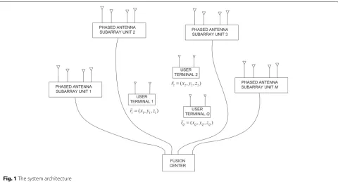
Our system uses a distributed antenna array to selectively estimate the position of an independent RF transmitter, Tx, based on its code sequence (known to the system). All the antennas, including the transmitting one, are dis-tributed indoors and are either stationary or slow-moving (see Fig.1). The slow-moving requirement is needed to allow for neglecting Doppler effects. The receiving anten-nas are grouped inM“subarrays.” The distances between the antennas within the same subarray are of the order of the carrier wavelength,λc.

Themth subarray hasLmantennas with positionsrm,l=

xm,l,ym,l,zm,l

,m∈ {1, 2,. . .,M}, andl∈ {1, 2,. . .,Lm}.

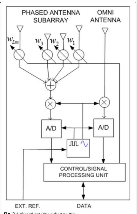
The signals from those antennas are inputs to a beam-former, which multiplies them by complex coefficients

wm,l that are electronically set in advance (see Fig. 2).

The output of the mth beamformer is IQ (in-phase quadrature-phase) demodulated and A/D (analog-to-digital) converted to obtain the (complex) samples of the

mth channel. Further, each subarray has an omnidirec-tional receiving antenna atrm,0 =

xm,0,ym,0,zm,0

with its own A/D converter. Thus, the digital signal processor (DSP) in the fusion center has access to 2Mchannels.

Another option is to have A/D converters and pro-cessing circuitry at the units. Then, they are digitally connected to the fusion center.

The Tx antenna is at an unknown positionr=(x,y,z), whereas the three-dimensional positions of all the other antennas in the system are known. All the receiving chan-nels are time, phase, and frequency synchronized to each other. Time synchronization between the Tx and our sys-tem is not required. However, it is assumed that they both use the same (known) carrier frequency. To perform the most accurate position estimation, each of the channels,

Fig. 2A phased antenna subarray unit

including the one of the Tx, must match the phase of its local carrier to its clock. With the matching, the car-rier phase would be 0 at each beginning of observation interval.

In summary, every antenna unit in the proposed sys-tem includes one omni antenna and one phased antenna array (two receiving channels are needed at each antenna unit). Thus, we have two functionally independent, mutu-ally synchronized distributed antenna systems in time and frequency.

2.1.2 Multistage/multiresolution searching and scanning strategy

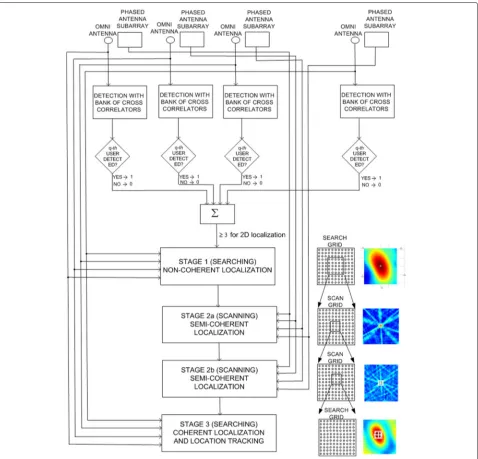
The system performs detection and location estimation of user transmitters in three stages, Fig.3. In stage 1, the sys-tem runs a numerically low-intensive algorithm to detect the presence of RF transmissions and to obtain approx-imate estapprox-imates of the transmitters’ locations. Only the omni antennas are employed in stage 1, and they can be used all the time. To start the estimation, the algorithm has to wait only for a single period of the Tx sequence. Each omni antenna channel has a bank of as many cross-correlators as there are user sequences of interest. When at least three cross-correlators detect the presence of a sequence sfor two-dimensional localization (or four for three-dimensional localization), the algorithm performs coarse localization of this user (with sequences) over a grid that spans the entire area of interest. The resulting inaccuracy of the estimated locations is expected to be of the order of 10λcor more.

In stage 2, another algorithm refines the search of the previous stage by scanning the area around the previous estimates using the subarrays. Since each subarray can only operate with a single set of coefficients wm,l at a

time, more than one observation period is needed for a single estimate. The length of the period corresponds to the period of the user sequence. Also, there must be time intervals between the periods so that the beamformers can change their coefficients.

Stage 2 can be split into steps 2a, 2b, etc., each cor-responding to beamformers with different beam widths, resolutions, and scan areas. The number of steps depends on the ratio of the resulting root-mean-squared error (RMSE) of stage 1 and the required RMSE of stage 2. The larger the ratio, the more steps should be used to keep the number of observation intervals down. The coefficients in stage 2a are chosen to create relatively wide (sector) beams for the subarrays in order to decrease the num-ber of points on the scan grid, while still providing an SNR (signal-to-noise-ratio) gain compared to that of the omnidirectional antennas. This translates into a smaller number of sequence periods required for estimation.

Fig. 3The block scheme of the multistage/multiresolution search strategy

area. Each scan point requires a new sequence period. The scan grid needs to be sufficiently fine so that the result-ing location error is belowλc. The overall purpose of this

stage is to shrink enough the search area so that in the third stage one can solve the so called ambiguity problem, discussed later in the text, which is inherent to the applied algorithm.

In stage 3, only one sequence period is needed and only the signals from the omni antennas are used. The algo-rithm in this stage relies on the phase relations among the different channels to make the most accurate esti-mates. The search grid is small but very fine because the resulting error is expected to be of the order ofλc/100 or

better. When the Tx is localized with this accuracy and it moves, it can be tracked by continuously running the same algorithm.

2.1.3 Signal model

The Tx prepares a periodic training signal in the following way. A complex sequences=[s0,s1,. . .,sN−1], assigned to a user, is repeated multiple times and D/A (digital-to-analog) converted with sampling frequencyνs. The

result-ing periodic continuous-time signal is s(t), where the time variabletin the mathematical model is normalized with 1/νs. For compatibility between the discrete-time

time values with 1/νsand frequencies withνsthroughout

the paper. The real and imaginary components ofs(t)are upconverted to the carrier frequencyνcwith quadrature

carriers. The resulting RF signal is periodic with period

N/νsand its bandwidth isB. The signals in all the channels

are sampled at the Nyquist rate, which impliesB=νs.

The RF signal of the Tx propagates atc=3×108m/s. The lth antenna in the mth subarray receives the signal whose baseband equivalent is

0 denotes the omni antenna associated with the appropri-ate subarray;am,l is an unknown real-valued attenuation

coefficient; ωc = 2πfc and fc = νc/νs are normalized

carrier frequencies in radians per sample and cycles per sample, respectively;t0is an unknown delay of the start of the transmission of a period of the Tx signal rela-tive to the receiving system’s time axis; τ_m,l = d_m,lνs/c

is the propagation delay from the Tx to the appropriate receiving antenna wheredm,l= r− rm,l;ηm,l(t)is

inde-pendent complex Gaussian noise in the frequency range

(−1/2, 1/2). The baseband equivalent of the signal at the output of themth beamformer is

um(t)=sm(t)+ηm(t), (3)

The discrete-time matrix baseband model derived from (1)–(5) is given by operator that also models the appropriate carrier phase

shift, and F is a modified DFT (discrete Fourier trans-form) matrix such thatF−1 = FH and whose rows are sorted by their corresponding natural RF frequencies. More formally,

, exp() is the element-by-element exponential function, and Diag{}is a diagonal matrix with the given elements on its main diagonal.

2.2 Direct position estimation algorithms

In this subsection, we describe algorithms for estimating the position of a user with a code sequences, where the algorithms have different levels of accuracy and numerical complexity. The algorithms are derived for a single-user scenario; however, if the code sequences of the other users are orthogonal tos, the algorithms can also be applied in multi-user settings. If the sequences are not orthogonal and the users are sufficiently separated from each other in space, the algorithms should still work well.

2.2.1 Coherent algorithms

First, we discuss coherent algorithms, which rely on dif-ferences of carrier phases among signals from different channels and on differences of complex envelopes. We point out that information about the Tx location is also present in the signal amplitudes; however, we will not use it here.

The coherent algorithms only use the signals from the omni antennas; therefore, the available data for process-ing include the time samplesum,0(n) for 1 ≤ m ≤ M, 0≤n≤N−1. We assume that the noises in the channels have the same power, which is known, so thatηm,0(n)has a circularly symmetric Gaussian probability density func-tion (PDF) with mean 0 and variance σ2, or ηm,0(n) ∼

CN0,σ2,∀m. In practice, if the noisy data have differ-ent powers, they can be scaled by differdiffer-ent factors to make this condition hold. The PDF of the observed data is

fC(u0)∝

M

m=1

exp−um,0−sm,02/σ2, (16)

where·denotes the Frobenius norm. We want to esti-mate the unknown parameters ofsm,0,∀m, from which we can estimate the location of Tx.

According to the ML method, we maximize the likelihood function (also given by (16)) with respect to the unknown parameters, a1,0,. . .,aM,0,t0,x,y,z

. This maximization is equivalent to the minimization of

M

g1=

Note that the propagation timesτm,0implicitly depend on the coordinates of the Tx,x,y,z.

The minimization can be first carried out over

am,0 (∀m) and then over(t0,x,y,z). For givent0,x, y,z,

Note that negative values are not allowed for the ampli-tude am,0 and that the function being minimized is a second-degree polynomial ofam,0. After substituting (18) in (17), we obtain the estimates oft0,x,y, andzfrom

The above steps represent the coherent ML algorithm. The search for the best values of(t0,x,y,z)must be very fine, but this would result in high numerical complexity. As an alternative, we propose a statistically suboptimal approach but numerically much more efficient. Without loss of generality, we select the first channel to be the ref-erence channel. In a preprocessing step, we estimate the total delay in that channel,t1=t0+τ1,0from

This maximization can further be simplified by breaking it down into three steps. First, we estimate an integer-valued delayt1,int, dismissing the carrier phase, from

t1,int=arg max

In the second step, we find a fractional, but still a rela-tively rough estimatet1,rby searching in a smaller interval, say, t1 ∈

t1,int−0.5,t1,int+0.5

, also dismissing the carrier phase and using (21), or

t1,r=arg max

In the third step, we estimate with the highest accuracy ˆ

t1, by searching in the smallest interval aroundt1,r, now relying also on the carrier phase and employing (20).

Finally, once we obtaint1, we estimate the location of Tx from

This is the algorithm we will use in stage 3 of the esti-mation process. Note that this final search grid does not include thet0 dimension and that the calculation of the first term in the sum (m = 1) can be omitted because it is constant. Also, in practice, channel 1 may sometimes have low SNR, and therefore, another channel should be selected as a reference.

One inherent disadvantage of the coherent algorithms is that there are many high and narrow lobes in the cri-terion function near the true location of the Tx. This is often referred to as the “ambiguity problem.” Stage 3 relies on stage 2 of the localization to correctly identify the main lobe from the side lobes.

Besides the ambiguity problem in the spatial domain, there is also an ambiguity problem in the estimation oft1 in the time domain. The resulting effect is an additional error which is an integer multiple of 1/fc. This error is

equal across the channels and (x,y,z). For narrowband signals, its impact on the localization accuracy is negligi-ble. For wideband signals, on average, this error is smaller than for narrowband signals.

2.2.2 Non-coherent algorithms

Now, we discuss algorithms that discard carrier phase dif-ferences between signals from different channels, unlike the coherent algorithms that exploit these phase differ-ences. The algorithms use the same data as the ones in Section 2.2.1; however, their criterion functions do not fluctuate nearly as much over(x,y,z)and as a result their estimates are much less accurate. Convenient conse-quences of this are that the search grid can be made much coarser and that the ambiguity problem does not exist.

We assume completely unknown phase terms in each channel,ψm,0, and write

sm,0=am,0ejψm,0FHDt0+τm,0Fs. (25)

_ψ1,0,. . .,ψM,0,t0,x,y,z

= arg max ψ_1,0,...,ψM,0 t0,x,y,z

M

m=1

Reejψm,0_uH

m,0FHDt0+τm,0Fs

2

.

(26)

We can find the solutions forψm,0 separately. Namely, for givent0,x,y,z, the solutions forψm,0are given by

ψm,0= −arg

uH_m,0FHDt0+τm,0Fs

, m=1, 2,. . .,M. (27)

When these solutions are substituted in (26), we opti-mize over(t0,x,y,z), or

t0,x,y,z

=arg max

t0,x,y,z M

m=1

uH_m,0FHDt0+τm,0Fs

2 . (28)

We refer to the algorithm based on the solutions in (27) and the optimization in (28) as the noncoherent ML algorithm.

We also propose a noncoherent ML algorithm with reduced computational complexity. As in the coherent algorithm, we first estimate the total delay in channel 1 and use the obtained estimate to search for the coordi-nates of Tx, or

(x,y,z)=arg max

x,y,z M

m=1

uH_m,0FHD_{τm,0−τ1,0+}t1Fs 2. (29)

This is the algorithm we will use in stage 1 of the esti-mation process. The first term in the sum is constant, so it can be omitted (the index mcan take just the values

2, 3,. . .,M). Also note that there is no need for the esti-matet1to be as accurate as in the implementation of the coherent algorithm. Therefore, one can skip step 3 of the method for estimatingt1accurately. Instead oft1, one can uset1,r.

2.2.3 Semi-coherent algorithms

The difference between the coherent and non-coherent algorithms is in the way how the summation in the cri-terion function is used; in the coherent algorithm, it is the real component of the sum that is applied whereas in the non-coherent algorithm, it is the absolute values of its terms that are exploited (cf. (24) and (29)). By tak-ing absolute values, the constant phase differences among channels are lost. We can use this idea to formulate a semi-coherent algorithm by taking the appropriate abso-lute values before summing over the channels (over m), but after summing over the antennas in each subarray (over l). In this way, the phase differences between the antennas of the same subarray are preserved, whereas the phase differences between subarrays are lost.

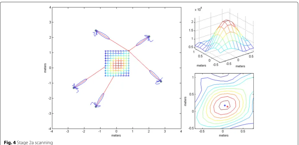
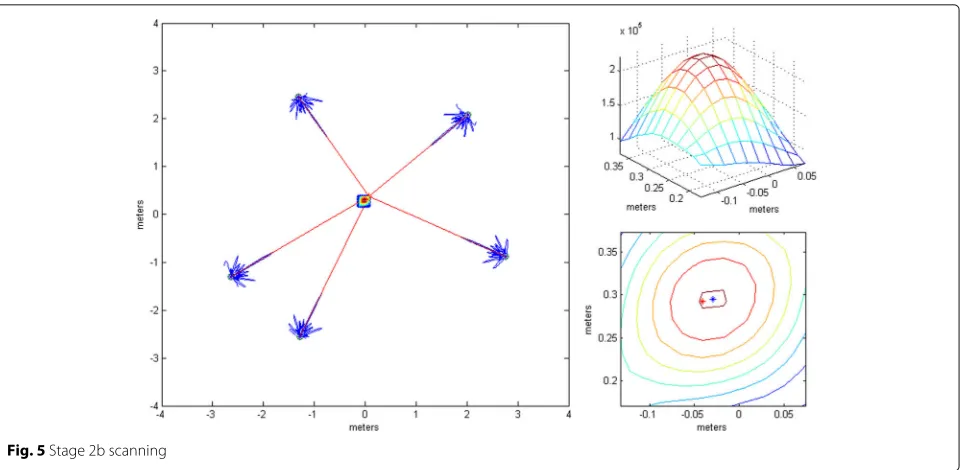
Let us choose a scan grid inside a given area of inter-est, see Figs. 4 and 5. Let rSGp be the position of the

pth point on the scan grid. Unlike the coherent and non-coherent algorithms, for each point on the scan grid, a newN-sample-long signal segment,u(mp),(∀m), is received

by the beamformers whose beams have been directed to this point. The beams are formed by setting their coeffi-cientswm,l. The 3 dB widths of the beams are chosen to

be greater than the distance between adjacent scan-grid points to avoid degradation due to the grid. The objective is to estimatepandt0by

Fig. 5Stage 2b scanning signal time delay matrix without a carrier phase shift, unlikeDτ. The position estimate of Tx is thenˆr= rSGpˆ.

As before, we can avoid estimatingt0by estimatingtm

for each omni antenna in preprocessing and then maxi-mizing overp, i.e.,

This is the algorithm we will use in stage 2 of the estima-tion process.

If the signals are narrowband, the expressions (30) and (31) reduce to (32) and (33), respectively:

3 Numerical results and discussion

This section provides numerical results obtained by the presented algorithms with Monte Carlo simulations for two scenarios—a LoS-only scenario and a multipath sce-nario. We experimented with two distributed receiver antenna array geometries for each of the two scenarios.

GeometryG1consists of five antenna subarrays, each sub-array having the geometry of an 18-element acoustic cam-era scaled down by a factor of 3 [39]. One omni antenna is added to the center of each subarray. The centers are in the plane,z=0. The omni antennas have the following coor-dinatesxandyin meters:(−2.20,−1.24),(0.18,−2.64),

(2.96,−1.06),(2.53, 2.21), and(−2.18, 2.24). They are rep-resented by white triangles in the figures in this section.

The positions of the subarrays were chosen by hand in order to be irregular. The distances between subarrays were selected to correspond to subarrays placed on the walls of a room. The subarrays have planar geometry in vertical plains, rotated around their vertical axes so that their broadside directions (approximately) point to the center of the area between subarrays (the room). Geom-etry G2is formed from G1 by scaling up by a factor of five the antenna positions in the subarrays with respect to their centers (omni antennas). The simulations were carried out using a known deterministic sequence, the first of the modulatable orthogonal sequences proposed in [40] for a given N. The parameters were as follows:

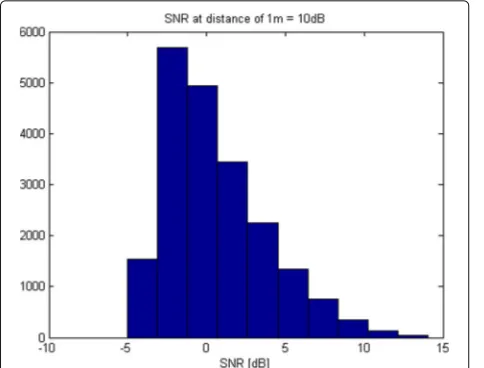
νc = 60 GHz B = 10 MHz, and SNR0 = 10 dB (if not stated otherwise), where SNR0 denotes the SNR in a virtual channel whose antenna is at a distance of 1 m from the transmitting antenna. Throughout this section, we assume that the signal power decreases with squared distance from the transmitter.

In the multipath scenario, we simulated a specular mul-tipath. We simulated only first-order reflected paths off four vertical planes (x = −2.4 m, y = −2.85 m,

LoS component power and the sum of reflected compo-nent powers (the Rice factor) of at least 10 dB. According to the ray-tracing method, the reflected components were modeled as if they were sent by virtual images of the Tx (w.r.t. the walls) according to the LoS model (7) (which includes a time shift, a carrier phase shift, and an attenu-ation). The reflected components were then phase shifted byπ, and their sum at each receiving antenna was scaled to get the specified Rice factor.

3.1 Qualitative characterization of the criterion functions

This subsection shows the qualitative behavior of the cri-terion functions of the respective algorithms for each of the three localization stages. The Tx was at(0, 0, 0), near the “center” of eitherG1orG2. Since stages 1 and 3 employ only omni antennas, the choice of subarray geometry does not matter. The criterion functions are shown over areas lying in the planez= 0. In Figs.6,7,8,9,10, and11, the true Tx location is marked by a circle with a cross and the estimated location by a square.

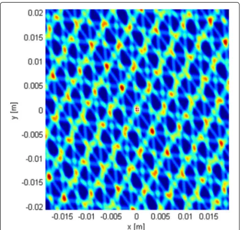
In order to localize the Tx with accuracy much better thanλc, we use the coherent algorithm. Its criterion

func-tion has high side lobes and requires a very fine search grid (see Fig. 6). Therefore, we cannot work with it immedi-ately, but instead we resort to a multistage/multiresolution search.

Figure7shows the LoS-only criterion function of stage 1 (given by (29)) over an area inside the antenna array for

N = 1024. The function does not have side lobes, it is not influenced by carrier phases, it is immune to phase synchronization errors, and it varies slowly across space, which suggests that a coarse grid can be used.

Fig. 6The criterion function of stage 3, given by (24) withN=1024

Fig. 7Criterion function of stage 1, given by (29) withN=1024

Figure8shows the LoS-only criterion function of stage 2 over an area inside the antenna array forG1forN=1024. We have also generated the corresponding criterion func-tion for N = 16, but it is not shown because it has the same shape. It also has no side lobes but shows more vari-ations across space compared to the criterion function of stage 1. This function offers better estimation accu-racy. Figure9shows the same results over a smaller area for geometryG2. The figures suggest that the plane wave

Fig. 9Criterion function of stage 2 forG2withN=1024

assumption would not be justified because of the size of subarray apertures.

Figure10shows the LoS-only criterion function of stage 3 for N = 1024 over an area around the transmitter spanning a little more than the main lobe. As the used algorithm is coherent (utilizes information in the phase of the carrier for localization), the criterion function has side lobes, separated by approximately 2λc/3. Since we use an

adaptive search grid in this stage, the algorithm finds the

Fig. 10Criterion function of stage 3, given by (24) withN=1024

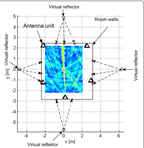
Fig. 11Criterion function for stage 2,G1, Rice factor 10 dB, and N=1024 with ray-tracing

peak of the lobe it has been initialized on (the initializa-tion point is the estimate obtained in stage 2). Clearly, to prevent the algorithm from converging to a side lobe, the localization in stage 2 must produce an estimate inside the main lobe of the criterion function of stage 3. In other words, if the localization error of stage 2 is smaller than approximately λc/3, the ambiguity problem is resolved,

because the displacement of the center of the main lobe in stage 3 due to noise is small compared to its width without noise.

Figure 11 shows the criterion function of stage 2 in the multipath scenario forN = 1024 over an area inside the antenna array forG1, along with wall positions and the “rays” from the ray-tracing method. The Rice factor was 10 dB. The figure shows that the localization algorithm is robust w.r.t. the multipath propagation since the lobes corresponding to the reflected rays cannot be seen. The criterion functions for stage 1 and 3 with multipath prop-agation are not given because they are almost identical to the LoS-only ones.

3.2 Quantitative characterization of the algorithms

In this subsection, we evaluate the accuracy of the algo-rithms of each stage. As performance metrics, we used both the MSE (mean squared error) and RMSE of the estimates.

Fig. 12Distribution of SNRs at the antennas for simulated Tx locations forSNR0=10 dB

The contour plots in the rest of the section were gen-erated over a Tx grid of 16×16 points that covers most of the area inside the array to show the error distribution across space. The grid has uniformly spaced points in the planez=0.

In Fig.13, we plotted the LoS-only RMSEs relative to the carrier wavelength,λc, for stage 1 forN = 1024. For

every Tx grid point, we performed 100 Monte Carlo runs and averaged out the results. Note that the accuracy is generally better near the first antenna because it is used as the reference antenna for estimatingt1. If the position

Fig. 13RMSE/λcfor stage 1 andN=1024

Fig. 14RMSE/_λcof stage 2 forG1andN=1024

estimate of this stage is far away from the reference antenna, another antenna can be adopted as the refer-ence and the process is repeated. Stage 3 could benefit from choosing a better reference antenna even more. The RMSE of stage 1 varies between 6 and 12λcin the given

area. These values determine how narrow the search grid in the next stage can be for a given Tx position, because

Fig. 16RMSE/λcof stage 2 forG2andN=1024

the grid should include the real Tx position. If the esti-mation errors have Gaussian distributions, the search grid for the next stage should span an area that is±2 standard deviations of the current stage along each dimension in order to include the real location with probability of 0.95.

The LoS-only RMSEs relative toλc for stage 2 for G1 andN = 1024 is shown in Fig. 14. Again, we ran 100

Fig. 17Probability of missing the main lobe in stage 3 due to the error in stage 2, forG2used in stage 2 andN=1024

Fig. 18RMSE/λcof stage 3 andN=1024 when the main lobe is not

missed

Monte Carlo simulations for every Tx grid point and computed from them the RMSEs. The same results but forG2, and N = 16 and N = 1024, are presented in Figs.15 and16. These results are better because of the increased space between the antennas in the subarrays.

10−7 10−6 10−5 10−4 10−3 10−2 10−1 0

0.1 0.2 0.3 0.4 0.5 0.6 0.7 0.8 0.9 1

miss−distance [m]

Probability

Main lobe G₂ init.

G₁ init.

10−4 10−3 10−2 10−1 100 101

0 0.1 0.2 0.3 0.4 0.5 0.6 0.7 0.8 0.9 1

miss−distance [λc]

Fig. 20Stage 3 error CDF curves for different initializations

The increased space produces “narrower beams,” i.e., bet-ter spatial selectivity. ForN = 1024 andG2, the RMSE is below λc/6 over a significant part of the area inside

the array. This allows the search in stage 3 to start some-where within the main lobe of its criterion function with a probability of 0.95. Thus, we can argue that the ambiguity problem is avoided with high probability. The simulations in which the analog beamformers had phase quantization with a resolution of 3◦were also carried out. The results are not shown here because they were almost identical to the ones without phase quantization.

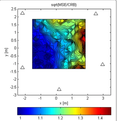
The LoS-only results for stage 3 forN =1024 are plot-ted in Figs.17,18, and19. In this experiment, for every Tx grid point, we had 1000 Monte Carlo runs. In Fig.17, we see how the probability of obtaining an estimate from a side lobe (or that the main lobe was missed) varies across the Tx grid. This probability depends on the estimate of stage 2 because the algorithm of stage 3 uses an adaptive grid that converges to the maximum of the lobe on which it has been initialized. Figure18shows the RMSE across the Tx grid provided that the main lobe has not been missed. As for stage 1, the effect of choosing the reference antenna can be seen (because the accuracy is better near the reference antenna). In this case, the obtained accuracy is of the order ofλc/100. For comparison reasons, we have

also run simulations for SNR0 = 20 dB, and the RMSE for the Tx at(0, 0, 0)isλc/963. In Fig.19, we observe the

statistical efficiency measured as the ratio of MSE and Cramér-Rao bound for the stage 3 algorithm when the

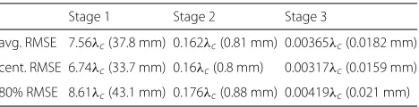
main lobe has not been missed. Figure20shows LoS-only CDF (cumulative density function) curves of the stage 3 localization error for N = 1024 for three cases: (1) the main lobe is not missed, (2) the stage 3 algorithm is ini-tialized by the results of the stage 2 algorithm forG2(see Fig.16), and (3) the stage 3 algorithm is initialized by the results of the stage 2 algorithm forG1(see Fig.14). The CDF curves were obtained for the same Tx grid as for the contour plots (e.g., Fig.13) with five runs for each grid point. As predicted, the algorithm in case (2) misses the main lobe only 2% of the time. On the other hand, the algorithm in case (3) misses the main lobe 78% of the time. For easier comparison of the numerical results for the LoS-only scenario, we provide them in Table1. The first row shows the RMSE averaged over the Tx grid, the sec-ond row the RMSE at a point near the center of the array (roughly (0, 0, 0)), and the third row the value not exceeded by the RMSE of 80% of the points on the Tx grid. The results are for the case when the main lobe in stage 3 is not missed.

Figure21shows CDF curves for different Rice factors for all three localization stages for N = 1024. For each

Table 1RMSEs for search/scan stages (G2andN=1024)

Stage 1 Stage 2 Stage 3

avg. RMSE 7.56λc(37.8 mm) 0.162λc(0.81 mm) 0.00365λc(0.0182 mm)

cent. RMSE 6.74λc(33.7 mm) 0.16λc(0.8 mm) 0.00317λc(0.0159 mm)

10−7 10−6 10−5 10−4 10−3 10−2 10−1 100 0

0.1 0.2 0.3 0.4 0.5 0.6 0.7 0.8 0.9 1

miss−distance [m]

Probability

LoS−only

LoS+NLoS (Rice f. 15 dB) LoS+NLoS (Rice f. 10 dB)

10−4 10−3 10−2 10−1 100 101 102

0 0.1 0.2 0.3 0.4 0.5 0.6 0.7 0.8 0.9 1

miss−distance [λ_c]

Fig. 21CDF curves of localization errors for different stages and Rice factors for SNR0=10 dB

stage, we show a CDF curve for LoS-only and Rice factor values of 15 and 10 dB. GeometryG2was used (in stage 2). Again, these results hold for outcomes when the main lobe in stage 3 is not missed. In stage 1, compared to the LoS-only curve, the error is increased roughly 2.5 and 4.3

times for Rice factors 15 and 10 dB, respectively. In stage 2, the error is increased 1.2 and 1.3 times. In stage 3, the error increase is 6 and 10 times. Stage 2 is the least affected by multipath propagation thanks to the beam directivity of the subarrays. The vertical line atλc/3 shows whether the

10−8 10−7 10−6 10−5 10−4 10−3 10−2 10−1 100

0 0.1 0.2 0.3 0.4 0.5 0.6 0.7 0.8 0.9 1

miss−distance [m]

Probability

LoS−only

LoS+NLoS (Rice f. 15 dB) LoS+NLoS (Rice f. 10 dB)

10−5 10−4 10−3 10−2 10−1 100 101 102

0 0.1 0.2 0.3 0.4 0.5 0.6 0.7 0.8 0.9 1

miss−distance [λ_c]

stage 2 estimate is within the main lobe of stage 3 or not. This is a critical value for solving the ambiguity problem. Even for a Rice factor of 10 dB, the ambiguity problem is solved 90% of the time.

Figure22shows the appropriate CDF curves for SNR0= 20 dB (instead of 10 dB as in Fig.21). As expected, the results for the LoS-only scenario are better. However, the results for the multipath environment are practically the same. Therefore, the adverse effect of multipath propaga-tion is greater for higher SNR values.

To summarize, as opposed to the existing methods men-tioned in Section1, which achieve a submeter localization accuracy, the proposed methods improve that accuracy to a small fraction of the carrier wavelength, which enables the shift from location-based services to location-based communication for dramatic improvement of a 5G system performance.

4 Conclusions

In this paper, we addressed indoor position estimation with a millimeter-wave massive MIMO system. We pro-posed an architecture with distributed antenna units, a multistage/multiresolution strategy, and three classes of localization algorithms that together achieve RMSE of up to three orders better than the carrier wavelength, and solve the ambiguity problem, inherent to coherent algorithms. In the LoS-only scenario, the localization error is by two to three orders better than the carrier wavelength, whereas in the specular multipath scenario, it is up to 10 times worse for realistic Rice factors, but still well below the carrier wavelength. The strat-egy does not require channel-state information and is applicable in multi-user scenarios, but requires domi-nant LoS propagation. The studied signal model is inher-ently wideband, and it assumes spherical wavefronts. The execution of the algorithms can be partially dis-tributed among the subarray units. The obtained accuracy allows the base station array to focus energy to the posi-tion of the localized user terminal on downlink and to receive its uplink signal emitted with decreased power. This can dramatically improve the overall capacity of the millimeter-wave massive MIMO system. An open issue is positioning of the BS antennas with accuracy greater than that of the localization, including the orientation of the subarrays.

Abbreviations

3GPP: 3rd Generation Partnership Project; 5G: 5th generation; A/D: Analog-to-digital; BS: Base station; CDF: Cumulative density function; DoA: Direction of arrival; CRB: Cramér-rao bound; D/A: Digital-to-analog; DFT: Discrete Fourier transform; DSP: Digital signal processor; IQ: In-phase quadrature-phase; LoS: Line-of-sight; MIMO: Multiple-input-multiple-output; ML: Maximum likelihood; MSE: Mean squared error; NLoS: Non-line-of-sight; PDF: Probability density function; RF: Radio frequency; RFID: Radio frequency identification; RMSE: Root mean squared error; RSS: Received signal strength; RSSI: Received signal strength indicator; SNR: Signal-to-noise-ratio; ToA: Time of arrival; Tx: Transmitter; UT: User terminal

Acknowledgements

This work was supported by national project TR32028 “Advanced Techniques for Efficient Use of Spectrum in Wireless Systems.”

Authors’ contributions

All authors read and approved the final manuscript.

Competing interests

The authors declare that they have no competing interests.

Publisher’s Note

Springer Nature remains neutral with regard to jurisdictional claims in published maps and institutional affiliations.

Author details

1_{School of Electrical Engineering, University of Belgrade, Belgrade, Serbia.} 2_{Innovation Center of School of Electrical Engineering, University of Belgrade,}

Belgrade, Serbia.3_{Department of Electrical and Computer Engineering, Stony} Brook University, New York City, NY, USA.

Received: 5 January 2018 Accepted: 22 May 2018

References

1. T Marzetta, Noncooperative cellular wireless with unlimited numbers of base station antennas. IEEE Trans. Wireless Commun.9(11), 3590–3600 (2010)

2. E Torkildson, U Madhow, M Rodwell, Indoor millimeter wave MIMO: feasibility and performance. IEEE Trans. Wireless Comunn.10(12), 4150–4160 (2011)

3. Z Pi, F Khan, An introduction to millimeter-wave mobile broadband systems. IEEE Commun. Mag.49(6), 101–107 (2011)

4. TS Rappaport, S Sun, R Mayzus, H Zhao, Y Azar, K Wang, GN Wong, JK Schulz, M Samimi, F Gutierrez, Millimeter wave mobile communications for 5G cellular: It will work! IEEE Access.1, 335–349 (2013)

5. EG Larsson, O Edfors, F Tufvesson, TL Marzetta, Massive MIMO for next generation wireless systems. IEEE Commun. Mag.52(2), 186–195 (2014) 6. AL Swindlehurst, E Ayanoglu, P Heydari, F Capolino, Millimeter-wave

massive MIMO: the next wireless revolution. IEEE Commun. Mag.52(9), 56–62 (2014)

7. RW Heath, N González-Prelcic Rangan, W Roh, A Sayeed, An overview of signal processing techniques for millimeter wave MIMO systems. IEEE J. Sel. Topics Signal Process.10(3), 436–453 (2016)

8. V Venkateswaran, AJ van der Veen, Analog beamforming in mimo communications with phase shift networks and online channel estimation. IEEE Trans. Signal Process.58(8), 4131–4143 (2010) 9. J Brady, N Behdad, AM Sayeed, Beamspace MIMO for millimeter-wave

communications: system architecture, modeling, analysis, and measurements. IEEE Trans. Antennas Propag.61(7), 3814–3827 (2013) 10. S Hur, T Kim, DJ Love, JV Krogmeier, TA Thomas, A Ghosh, Millimeter wave

beamforming for wireless backhaul and access in small cell networks. IEEE Trans. Commun.61(10), 4391–4403 (2013)

11. A Alkhateeb, J Mo, N Gonzalez-Prelcic, RW Heath, MIMO precoding and combining solutions for millimeter-wave systems. IEEE Commun. Mag. 52(12), 122–131 (2014)

12. S Han, I Chih-Lin, Z Xu, C Rowell, Large-scale antenna systems with hybrid analog and digital beamforming for millimeter wave 5G. IEEE Commun. Mag.53(1), 186–194 (2015)

13. J Li, L Xiao, X Xu, S Zhou, Robust and low complexity hybrid beamforming for uplink multiuser mmwave MIMO systems. IEEE Commun. Lett.20(6), 1140–1143 (2016)

14. JC Chen, Hybrid beamforming with discrete phase shifters for millimeter-wave massive MIMO systems. IEEE Trans. Veh. Technol.66(8), 7604–7608 (2017)

15. A Guerra, F Guidi, D Dardari, On the impact of beamforming strategy on mm-wave localization performance limits. Presented at 2017 IEEE Int. Conf. Commun. Workshops, Paris, 21-25 May 2017

17. AF Molisch, VV Ratnam, S Han, Z Li, SLH Nguyen, L Li, K Haneda, Hybrid beamforming for massive MIMO: A survey. IEEE Commun. Mag.55(9), 134–141 (2017)

18. TS Rappaport, F Gutierrez, E Ben-Dor, JN Murdock, Y Qiao, JI Tamir, Broadband millimeter-wave propagation measurements and models using adaptive-beam antennas for outdoor urban cellular

communications. IEEE Trans. Antennas Propag.61(4), 1850–1859 (2013) 19. N Iqbal, C Schneider, J Luo, D Dupleich, RS Thöma, Modeling of

directional fading channels for millimeter wave systems. Presented at 2017 IEEE 86th Veh. Technol. Conf. (VTC Fall), Toronto, 24-27 Sept 2017 20. N Iqbal, J Luo, Y Xin, R Müller, S Haefner, RS Thöma, Measurements based

interference analysis at millimeter wave frequencies in an indoor scenario. Presented at 2017 IEEE Globecom, Singapore, 4-8 Dec 2017 21. TS Rappaport, JN Murdock, F Gutierrez, State of the art in 60-Ghz

integrated circuits and systems for wireless communications. Proc. IEEE. 99(8), 1390–1436 (2011)

22. W Roh, JY Seol, J Park, B Lee, J Lee, Y Kim, Y Cho, K Cheun, F Aryanfar, Millimeter-wave beamforming as an enabling technology for 5G cellular communications: theoretical feasibility and prototype results. IEEE Commun. Mag.52(2), 106–113 (2014)

23. S Malkowsky, J Vieira, L Liu, P Harris, K Nieman, N Kundargi, IC Wong, F Tufvesson, V Öwall, O Edfors, The worlds first real-time testbed for massive MIMO: Design, implementation, and validation. IEEE Access.5, 9073–9088 (2017)

24. R Di Taranto, S Muppirisetty, R Raulefs, D Slock, T Svensson, H Wymeersch, Location-aware communications for 5G networks: how location information can improve scalability, latency, and robustness of 5G. IEEE Signal Process. Mag.31(6), 102–112 (2014)

25. K Witrisal, P Meissner, E Leitinger, Y Shen, C Gustafson, F Tufvesson, K Haneda, D Dardari, A Molisch, A Conti, MZ Win, High-accuracy localization for assisted living: 5G systems will turn multipath channels from foe to friend. IEEE Signal Process. Mag.33(2), 59–70 (2016) 26. M Vari, D Cassioli, mmWaves RSSI indoor network localization. Presented

at 2014 IEEE Int. Conf. Commun. Workshops (ICC), Sydney, 10-14 June 2014

27. V Savic, EG Larsson, Fingerprinting-based positioning in distributed massive MIMO systems. Presented at IEEE 82nd Veh. Technol. Conf. (VTC Fall), Boston, 6-19 Sept 2015

28. N Garcia, H Wymeersch, EG Larsson, AM Haimovich, M Coulon, Direct localization for massive MIMO. IEEE Trans. Signal Process.65(10), 2475–2487 (2017)

29. T Wei, X Zhang, mTrack: high-precision passive tracking using millimeter wave radios. Presented at (2015) 21st Annual Int. Conf. Mobile Comput. Netw. Mobicom ’15, Paris, 7-11 Sept 2015

30. A Guerra, F Guidi, D Dardari, Position and orientation error bound for wideband massive antenna arrays. Presented at 2015 IEEE Int. Conf. Commun. Workshops (ICC), London, 8-12 June 2015

31. A Shahmansoori, G Garcia, G Destino, G Seco-Granados, H Wymeersch, 5G position and orientation estimation through millimeter wave MIMO. Presented at (2015) IEEE Globecom Workshops, San Diego, 6-10 Dec 2015 32. M Koivisto, M Costa, J Werner, K Heiska, J Talvitie, K Leppänen, V Koivunen,

M Valkama, Joint device positioning and clock synchronization in 5G ultra-dense networks. IEEE Trans. Wireless Commun.16(5), 2866–2881 (2017)

33. M Koivisto, A Hakkarainen, M Costa, P Kela, K Leppänen, M Valkama, High-efficiency device positioning and location-aware communications in dense 5G networks. IEEE Commun. Mag.55(8), 188–195 (2017) 34. J Werner, J Wang, A Hakkarainen, D Cabric, M Valkama, Performance and

Cramer-Rao bounds for DoA/RSS estimation and transmitter localization using sectorized antennas. IEEE Trans. Veh. Technol.65(5), 3255–3270 (2016)

35. M Scherhäufl, M Pichler, A Stelzer, UHF RFID localization based on phase evaluation of passive tag arrays. IEEE Trans. Instrum. Meas.64(14), 913–922 (2015)

36. M Oispuu, U Nickel, 3D passive source localization by a multi-array network: Noncoherent vs.coherent processing. Presented at Int. ITG Workshop Smart Antennas, Bremen, 23-24 Feb 2010

37. N Hadaschik, B Sackenreuter, M Schäfer, M Faßbinder, Direct positioning with multiple antenna arrays. Presented at (2015). Int. Cong. Indoor Posit. Indoor Navig. (IPIN), Bremen, 13-16 Oct 2015

38. J Lee, E Tejedor, K Ranta-aho, H Wang, K Lee, E Semaan, E Mohyeldin, J Song, C Bergljung, S Jung, Spectrum for 5G: Global status, challenges, and enabling technologies. IEEE Commun. Mag.56(3), 12–18 (2018) 39. PULSE Beamforming System with 18-channel sector wheel array based

on beamforming type 8608 Bruel Kjoer Product information.https:// www.bksv.com/~/media/literature/Product%20Data/bn1467.ashx. Accessed 30 May 2018

40. N Suehiro, M Hatory, Modulatable orthogonal sequences and their application to SSMA systems. IEEE Trans. Inf. Theory.34(1), 93–100 (1988) 41. H Xu, V Kukshya, TS Rappaport, Spatial and temporal characterization of