FULL PAPER
Time-lapse inversion of one-dimensional
magnetotelluric data
Dennis Conway
*, Graham Heinson, Nigel Rees and Joseph Rugari
Abstract
We present a new tool for modelling time-lapse magnetotelluric (MT) data, an emerging technique for monitoring changes in subsurface electrical resistivity. Time-lapse MT data have been acquired in various settings, including sites of hydraulic fracturing, dewatering and sequestration. It has been shown in other geophysical techniques that the most effective way to model lapse data is with simultaneous inversion, which uses information from all time-steps to produce models with higher accuracy and fewer artefacts. We introduce this method to model time-lapse 1D MT data. As with a standard MT inversion, our routine penalises spatial roughness at each time-step, however we also introduce temporal regularisation. The inversion is simple to apply, requiring only the ratio between regularisation parameters and the desired level of misfit from the user. The algorithm is tested on both synthetic data, and a case study. We find that in the synthetic example our inversion successfully retrieves the main characteristics of the test model and introduces minimal artefacts, even in the presence of significant noise. We also test the effect of chang-ing the ratio of regularisation parameters. In the case study, we produce an easily interpretable model that compares favourably with previous inversions of the synthetic data. We conclude that time-lapse modelling of 1D MT data can be a valuable tool for imaging subsurface change.
Keywords: Magnetotellurics, Time-lapse, Inversion
© The Author(s) 2018. This article is distributed under the terms of the Creative Commons Attribution 4.0 International License (http://creativecommons.org/licenses/by/4.0/), which permits unrestricted use, distribution, and reproduction in any medium, provided you give appropriate credit to the original author(s) and the source, provide a link to the Creative Commons license, and indicate if changes were made.
Open Access
*Correspondence: dennis.conway@adelaide.edu.au
School of Physical Sciences, University of Adelaide, North Terrace, Adelaide, Australia
Introduction
In recent years, the magnetotelluric method (MT) has been increasingly used as a cost-effective technique for subsurface resistivity monitoring (see Rees et al. 2016, for a general introduction). As this is a relatively new application for MT, there are few modelling tools avail-able. Peacock et al. (2012) have used differences in MT phase tensors to qualitatively interpret resistivity changes due to fluid injection in an enhanced geothermal system (EGS) at Paralana, South Australia. This technique has also be used by Didana et al. (2017) interpreting change at the Habernero EGS. Recent work includes parameteris-ing resistivity changes as a three-dimensional (3D) plume structure and inverting using Markov Chain Monte Carlo (Rosas-Carbajal et al. 2015). Another approach has been to use 1D layer-stripping, where the effect of over-lying structures is removed to model the time-varying
magnetotelluric responses at depth (Ogaya et al. 2016). Standard MT modelling tools such as inversion can also be adapted, for example Rees et al. (2016) use cascading two-dimensional (2D) inversions to model a coal-seam gas depressurisation, where the results from the pre-injection inversion are used as a prior-model for the post-injection. An improvement on cascaded inversion has been implemented by Rosas-Carbajal et al. (2012), where differenced 2D MT inversions have achieved high accu-racy by subtracting the prior-model response from all data and reducing the data error. High-accuracy simul-taneous time-lapse 1D MT inversions have also been approximated using 2D MT codes (e.g. Rees et al. 2016; Didana et al. 2017); however, this approximation leads to small errors in the calculation of the forward-model and hence inversion result.
Page 2 of 9 Conway et al. Earth, Planets and Space (2018) 70:27
time-lapse ERT data gives a superior result compared to independent inversions, cascading inversions or differ-enced inversions. Their preferred technique was a special case of the 4D algorithm of Kim et al. (2009), which has also successfully been applied to gravity (Karaoulis et al.
2013a), induced polarisation (Karaoulis et al. 2013b), and seismic tomography (Karaoulis et al. 2015). This tech-nique has not yet been presented for magnetotelluric inversion.
We present an implementation of a simple time-lapse algorithm to simultaneously invert 1D MT monitoring data. Firstly, we present the results from synthetic inver-sions of 1D magnetotelluric data to test the validity of the algorithm. We then present inversions from a case study of data from a coal-seam gas production survey (Rees et al. 2016).
Inversion method
The algorithm is an Occam style inversion (Constable et al. 1987), seeking to find the model which fits the data to a desired level whilst introducing the least amount of structure—in this case in both temporal and spatial domains. We seek to find the model (m) which minimises
the model roughness (R(m)) subject to the constraint
It is more convenient to express the misfit in terms of root-mean-square error (RMS), given by
The model roughness is the sum of regularisation in both spatial (S) and temporal (T) directions, weighted by a fac-tor β:
The temporal regularisation is given by the squared sum of the model changes in time:
minimize
and the spatial regularisation by the sum of second deriv-atives at each time slice:
The optimisation is performed using the Sequential Least SQuares Programming (SLSQP) algorithm available in scipy (Jones et al. 2001), which is based on the algorithm by Kraft and Schnepper (1989). The algorithm does not require any tradeoff parameter between data misfit and smoothing, as this is encapsulated in the target RMS. Data are read into the program using the mtpy module (Krieger and Peacock 2014).
Due to the efficiency of the 1D MT algorithm, which is calculated analytically, the model readily reaches an acceptable misfit within a few iterations. Subsequent iter-ations reduce the roughness of the model.
Synthetic study
Numerical data are first used to study the results of the time-lapse MT algorithm. The data are produced from a model of an idealised resistivity change at a single site for a coal-seam gas pump into a shallow aquifer. The initial resistivity is a 10 m halfspace. At survey day 4 a sharp
change occurs at a depth of 665–958 m, with the resistiv-ity dropping to 2 m. The input model for the synthetic
study is shown in Fig. 1.
Magnetotelluric impedance data are produced at 17 frequencies ranging from 0.14 to 6.26 Hz. The data were computed using the standard analytic 1D forward algorithm. The 1D assumption is valid if the resistiv-ity changes are sufficiently laterally continuous, which we would expect for changes in a lateral coal-bed. The assumption is not perfect however, as 3D effects would be present during the development of the resistivity front. The data were then contaminated with 5% Gauss-ian random noise on the impedance tensor, which is a reasonably high estimate of the errors expected in field operations. The data errors were fixed at 5%.
The inversion was conducted with a RMStarget of 1.0.
Smaller target RMS values result in overfitted models which mapped noise in the data as temporal change, whilst larger target RMS values underfit the change in the data. The β value, which weights the relative
For each inversion the target RMS was achieved within 5 iterations, however additional smoothing iterations were run, with a total of 100 iterations for each inversion.
Results and discussion
Figure 2 shows the resistivity for three synthetic inver-sions with varying ratios of temporal smoothing to spa-tial smoothing. On the left panels the absolute resistivity is shown, and on the right panels the change in resistivity relative to the initial resistivity is displayed.
The main feature in common to all three figures is the strong decrease in conductivity from day 2–3 onwards. In each inversion, the change is diffusively spread out across multiple layers, with the amount of spread dependent on the value for β. The diffusive spreading is most evident
with the smallest β value in Fig. 2a, and the largest value
of β in Fig. 2c has the changes confined to almost a single
layer.
Compared to the input model, each inversion model underestimates the change in the data. The relative change in the input model is an 80% drop over two lay-ers, whereas the three inversion models have drops in the order of 50–60%. The extent of the conductive change is overestimated by the β =100 model and underestimated
by the β=10, 000 model, with the middle β=1000
model providing a fairly accurate image. With increas-ing β the models also become rougher spatially. In the β=10, 000 scenario, for example, the model changes
from 1 to 100 m between three layers.
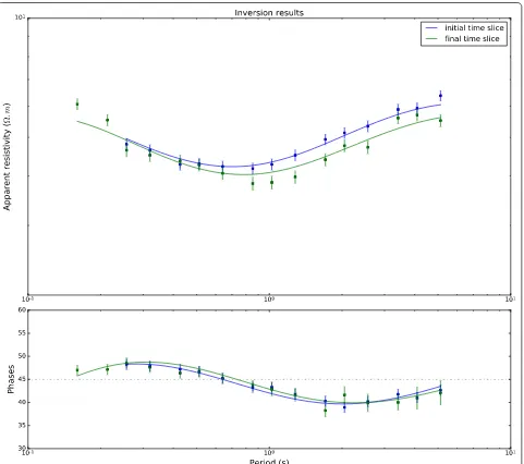
Example model fit curves from the first and final days are overlain in Fig. 3 for the β=1000 inversion, plotted
alongside the synthetic data used in the tests. The curves show that a good fit to the data is achieved at conver-gence. They also highlight the substantial change in the synthetic data due to the resistivity changes.
The inversions were reasonably accurate in terms of the absolute resistivities and the relative changes in resis-tivity. The smaller β value, however, spread the changes
out over a large spatial area. The algorithm will prefer-ence changes over as many layers as possible for two rea-sons. Firstly, the temporal roughness is calculated on the square of the change in any one layer, which means that it is preferable to spread changes over multiple layers if pos-sible. Secondly, and more importantly, the entire model is smoothed in the spatial dimension. The lowest β
param-eter resulted in a less concentrated area of change, with smaller changes spread over a greater area. The highest
β weighting gave a stronger concentration of change and
a smaller overall change in resistivity. The model, how-ever, became rougher in the spatial dimension leading to improbable absolute resistivities.
It is worth noting that the inverted models accurately pick the time when the resistivity change occurs. There is a slight change in resistivity before the inversion; however this change is unavoidable as the small data misfit which it introduces is offset by the improved tem-poral smoothing. If a priori information exists regarding
Page 4 of 9 Conway et al. Earth, Planets and Space (2018) 70:27
b a
c
Fig. 2 Inversion of synthetic model results. Inversion results for synthetic inversions using the parameters a β=100, b β=1000 and c β=10, 000.
the time tc when a resistivity change occurs, it can be
included by restricting all temporal change for t<tc. Case study
An example from a coal-seam gas field is used to fur-ther examine the algorithm. A coal-seam gas monitoring experiment is ideal to test the 1D time-lapse MT algo-rithm, as changes occur at shallow depths where the MT
response is better approximated by a 1D algorithm, and we expect any changes to be laterally continuous through the coal seam.
We use time-lapse MT data from a 2013/2014 sur-vey of a coal-seam gas field in the Surat Basin, Queens-land, Australia (Rees et al. 2016). Data for this survey were collected along two lines near several produc-tion wells. The wells extracted both water and gas from
Page 6 of 9 Conway et al. Earth, Planets and Space (2018) 70:27
depths of 400–700 m, and a resulting resistivity change was observed by Rees et al. (2016) in differenced MT inversions.
A schematic of the survey design is shown in Fig. 4, which also features production well locations. Site 105
was used for our inversion, which is the same site used for the 1D inversions in Rees et al. (2016). Data were used from 10 days between January 23, 2014 and February 19, 2014. The site is nearby the most active production well and had reasonable data quality during these days. MT data are taken from the YX mode as these are of higher quality than the XY mode data.
Identical to the synthetic study, the data have 17 fre-quencies ranging from 0.14 to 6.26 Hz. We invert these data using the presented time-lapse algorithm. We use parameters RMStarget=1.0, β =1000 and an error floor
of 2%. The inversion is run for 100 iterations and com-pleted within 20 min on a 4 core machine.
Results and discussion
The inversion resistivity model is shown in Fig. 5, with the resistivity differences shown in the same figure. A slight reduction in resistivity between 500 and 700 m begins on day 9 and slowly increases with time, culminating with a drop of roughly 15% in resistivity by the final day. There is also a slight (≈ 5%) increase in resistivity in the area between
100 and 500 m. Finally, there is also a reduction in resistiv-ity at depth; however, this is smaller than the resistivresistiv-ity drop in the higher zone. Notably this would be near the penetra-tion depth of the data, and would be less constrained than the other areas of the model. The entire model resistivity is between 1.25 and 16 m. When considering the
commence-ment date of pumping, shown as a dashed line in Fig. 5, we see that the resistivity changes occur slightly before the com-mencement of dewatering. In the synthetic model, temporal
Fig. 4 Schematic of survey extents. A schematic of the site used for inversion in the case study. Site 105 (highlighted) was one of the clos-est sites to the active pump well W4, and the most likely candidate for resistivity change. Electric field data were collected at each e-logger site, and MT responses calculated using the magnetic field data at the single b-logger site
a b
changes were smoothed by the algorithm to include dates before the change in the target model, and we would suggest that the same phenomenon is occurring here.
Looking at the fit of the response curves in Fig. 6, we see that the model slightly underfits some of the changes in the MT data. This is expected as the algorithm introduces the minimum change required to fit the data. This would place the estimations of 15% change in resistivity as conservative and shows the importance of obtaining high-quality data, as tighter error bars would lead to stronger changes in resistiv-ity. Notably there is a significant dip in the model fit curves between the first (in blue) and final (in green) time slices.
The most important area to consider in interpretation is the area of the resistivity decrease between 500 and 700 m, as the other resistivity changes in the model are much smaller and should not be overinterpreted. There seems to be a strong link between the start of the resis-tivity change and the dewatering event at W4. There is no gas extraction during this time. Hence, our new model would agree with the interpretation in Rees et al. (2016) that the changes are due to the increased perme-ability of dewatered coal-seams, potentially due to the reduction in the coal matrix as gas is released from the matrix.
Page 8 of 9 Conway et al. Earth, Planets and Space (2018) 70:27
Unlike the synthetic example, the changes in the model were slow, with a build up to the maximum change in the final day included in the inversion. This would lead us to believe that resistivity changes resulting from coal-seam gas pumping are related not just to the rate of pumping, but also the amount of material that has been removed from the pores.
Conclusion
We presented a simple time-lapse inversion of 1D MT data, which we tested on synthetic data and case-study data. Both inversions resulted in defined areas of resistiv-ity change with few artefacts in the models. The synthetic inversion obtained resistivity changes which slightly underestimated the changes in the input model; however, it accurately retrieved spatial and temporal locations, as well as absolute resistivities. We investigated the effect of the weighting parameter β between spatial and temporal
smoothing and showed that there is a tradeoff between models which are overly sharp spatially and models which overestimate the extent of the resistivity change. We also showed results from applying the algorithm to a case study with coal-seam gas MT data. The inversion resulted in small changes in the area of the coal-seams.
Compared to other modelling techniques, our algo-rithm has several advantages. Full 3D modelling is highly computationally intensive. A 1D approximation is simple to compute, which leads to a rapidly converging model. This allows the modeller to trial several parameters and select the best model. It also allows a large amount of data to be inverted at once—it is feasible to invert data from each day for several months, which would result in an extremely large model space in 3D. Compared to inde-pendent inversions, or time-lapse inversions using 2D MT codes as approximations, it has previously been shown that simultaneous inversion results in a model with fewer artefacts and stronger constraints on areas of change.
One of the disadvantages of the technique is that it is unable to fit any 2D or 3D aspects of the data. Further work could expand the technique into higher spatial dimensions, or to deal with anisotropy. It would be useful to extend the inversion into 3D space and incorporate all data into the inversion; however, the long processing times of higher-dimensional MT forward codes would make the resulting code extremely computationally intensive.
Abbreviations
MT: magnetotellurics; 1D: one-dimensional; RMS: root-mean-squared error.
Authors’ contributions
DC performed algorithm development and testing with help from GH and JR. NR helped in the case-study test by assisting with the data selection and mod-elling. All authors read and approved the final manuscript.
Acknowledgements
We would like to thank QGC Pty Limited for their funding of the data collec-tion, as well The Australian Geophysics Observing System and AuScope for providing the instrumentation. We thank S. Rana, G. Hicks, P. McKelvey and A. Smart for their help with field logistics, and S. Schnaidt, G. Boren, A. Tullis, B. Warren, S. MacMillan and C. Matthews for their assistance in field work. Finally, S. Carter and O. Putland and thanked for their help with data processing.
Competing interests
The authors declare that they have no competing interests.
Availability of data and materials
Included in supplementary material.
Consent for publication
Not applicable.
Ethics approval and consent to participate
Not applicable.
Funding
Not applicable.
Publisher’s Note
Springer Nature remains neutral with regard to jurisdictional claims in pub-lished maps and institutional affiliations.
Received: 28 August 2017 Accepted: 29 January 2018
References
Constable S, Parker R, Constable C (1987) Occam’s inversion: a practical algo-rithm for generating smooth models from electromagnetic sounding data. Geophysics 52(3):289–300. https://doi.org/10.1190/1.1442303
Didana YL, Heinson G, Thiel S, Krieger L (2017) Magnetotelluric monitoring of permeability enhancement at enhanced geothermal system project. Geothermics 66:23–38. https://doi.org/10.1016/j.geothermics.2016.11.005
Hayley K, Pidlisecky A, Bentley LR (2011) Simultaneous time-lapse electri-cal resistivity inversion. J Appl Geophys 75(2):401–411. https://doi. org/10.1016/j.jappgeo.2011.06.035
Jones E, Oliphant T, Peterson P et al (2001) SciPy: open source scientific tools for python. http://www.scipy.org/. Accessed 10 Mar 2017
Karaoulis M, Revil A, Minsley B, Todesco M, Zhang J, Werkema DD (2013a) Time-lapse gravity inversion with an active time constraint. Geophys J Int 196(2):748–759
Karaoulis M, Revil A, Tsourlos P, Werkema DD, Minsley BJ (2013b) IP4DI: a software for time-lapse 2D/3D DC-resistivity and induced polarization tomography. Comput Geosci 54:164–170. https://doi.org/10.1016/j. cageo.2013.01.008
Karaoulis M, Werkema DD, Revil A (2015) 2D time-lapse seismic tomography using an active time-constraint (ATC) approach. Lead Edge 34(2):206– 212. https://doi.org/10.1190/tle34020206.1
Kim JH, Yi MJ, Park SG, Kim JG (2009) 4-D inversion of DC resistivity monitoring data acquired over a dynamically changing earth model. J Appl Geophys 68(4):522–532. https://doi.org/10.1016/j.jappgeo.2009.03.002
Kraft D, Schnepper K (1989) SLSQP—a nonlinear programming method with quadratic programming subproblems. DLR, Oberpfaffenhofen Krieger L, Peacock JR (2014) MTpy: a python toolbox for magnetotellurics.
Comput Geosci 72:167–175
Ogaya X, Ledo J, Queralt P, Jones AG, Marcuello l (2016) A layer stripping approach for monitoring resistivity variations using surface magnetotel-luric responses. J Appl Geophys 132:100–115. https://doi.org/10.1016/j. jappgeo.2016.06.014
Rees N, Carter S, Heinson G, Krieger L, Conway D, Boren G, Matthews C (2016) Magnetotelluric monitoring of coal-seam gas and shale-gas resource development in Australia. Lead Edge 35(1):64–70. https://doi. org/10.1190/tle35010064.1
Rosas-Carbajal M, Linde N, Kalscheuer T (2012) Focused time-lapse inversion of radio and audio magnetotelluric data. J Appl Geophys 84:29–38. https:// doi.org/10.1016/j.jappgeo.2012.05.012