R E S E A R C H
Open Access
Unsupervised joint deconvolution and
segmentation method for textured images:
a Bayesian approach and an advanced
sampling algorithm
Cornelia Vacar and Jean-François Giovannelli
*Abstract
The paper tackles the problem of joint deconvolution and segmentation of textured images. The images are composed of regions containing a patch of texture that belongs to a set ofKpossible classes. Each class is described by a Gaussian random field with parametric power spectral density whose parameters are unknown. The class labels are modelled by a Potts field driven by a granularity coefficient that is also unknown. The method relies on a hierarchical model and a Bayesian strategy to jointly estimate the labels, theKtextured images in addition to
hyperparameters: the signal and the noise levels as well as the texture parameters and the granularity coefficient. The capability to estimate the latter is an important feature of the paper. The estimates are designed in an optimal manner as a risk minimizer that yields the marginal posterior maximizer for the labels and the posterior mean for the rest of the unknowns. They are computed based on a convergent procedure from samples of the posterior obtained through an advanced MCMC algorithm: Perturbation-Optimization step and Fisher Metropolis-Hastings step within a Gibbs loop. Various numerical evaluations provide encouraging results despite the strong difficulty of the problem.
Keywords: Segmentation, Deconvolution, Texture, Bayes, Unsupervised learning, Potts, Sampling, Optimization
1 Introduction: motivation and state of the art This paper addresses the complex problem of textured image segmentation that is a subject of importance in various applications [1, 2] (see also [3, 4]). In practice, observations are often affected by blur (due to finite reso-lution of observation systems) and by noise (due to various sources of error). However, existing approaches do not account for these issues and focus only on segmenta-tion. On the contrary, this paper addresses the problem of textured image segmentation from indirect (blurred and noisy) observations. It tackles the problem of joint deconvolution-segmentation of textured images, and to the best of our knowledge, no other paper has done any work in this area.
Image segmentation is a computer vision/image pro-cessing problem [5] consisting in partitioning an image
*Correspondence:[email protected]
IMS (Univ. Bordeaux, CNRS, BINP), Cours de la Libération, 33400 Talence, France
into groups of adjacent pixels that have a certain homo-geneity property (grey level, colour or texture) or that compose an object of interest. Since the problem has been of great interest for decades, the literature is extensive.
The most straightforward segmentation method is
thresholding; however, it is seldom applicable, since it is only adapted for piecewise constant images, not affected by blur or noise. In the class of region growing meth-ods, Zhang et al. [6] present a seeded image segmentation based on a heat diffusion process, Ugarriza et al. [7] describe an unsupervised region growing and multires-olution merging algorithm and Alpert et al. [8] present a bottom-up aggregation approach. Partial differential equation-based techniques have also been employed. For instance, Chan and Mulet [9] introduce an active contour without edges method for object segmentation, based on level sets, curve evolution, and the Mumford-Shah model. As for the watershed approach, Malik et al. [10] present a normalized cut approach relying on a local measure of similarity of the textural features in a neighbourhood
of the pixel, while Grady [11] uses a small number of predefined labels and computes a probability for each unlabelled pixel. The final label is the one maximizing this probability. Sinop and Grady [12] unify the graph cuts and the random walker methods in a common
frame-work, based onLqnorms minimization for seeded image
segmentation.
One of the first approaches for textured image
seg-mentation[13] is based on using as texture features the moments of the image, computed on small windows. The more recent method in [14] consists in computing features based on the Discrete Wavelet Transform of blocks of the image, evaluating the difference between these features on adjacent blocks and processing to obtain a one-pixel thick contours. This method does not provide a label field; thus, it gives no information about which texture belongs to which region. Another method providing texture edges [15] uses active contours and the patch-based approach for texture analysis. Textured image segmentation is also achieved in [16], based on features extracted from the Fourier transform of the learning textures. A significant method for image segmentation based on both grey level (intervening contour framework) and texture (textons) is presented in [10]. The segmented image is obtained
using a normalized cut approach. Mobahi et al. [17]
model a homogeneous textured region of an image by a Gaussian density and the region boundaries by adap-tive chain codes. The segmentation is obtained using a clustering process. Another approach devoted to strongly resembling textures is given in [18]. The goal is to accu-rately characterize the textures, and this is achieved by combining a collection of statistics and filter responses. This local information is then used in an aggregation process to determine the segmentation. A three-stage seg-mentation method is presented in [19] and relies on char-acterizing both textured and non-textured regions using local spectral histograms. Texel-based image segmenta-tion is achieved in [20] by identifying the modes in the probability density function of region properties.
A very significant class of segmentation methods relies on aprobabilisticmodel-based formulation. Geman et al. [21] present an approach for image partitioning into homogeneous regions and for locating edges based on dis-parity measures. In [22], an image segmentation method is developed based on Monte Carlo Markov Chain (MCMC) and theK adventurers algorithm by integrating cluster-ing and edge detection in the proposal probabilities. Deng
and Clausi [23] introduced a weighted Markov random
field model that estimates the model parameters and thus performs unsupervised image segmentation. Among the probabilistic methods, the graph partitioning approach is very popular. Felzenszwalb and Huttenlocher [24] uses a graph-based image model and measures the evidence for a boundary between two regions, while Boykov and
Funka-Lea [25] describe the basic framework for efficient object extraction from multi-dimensional image data using graph cuts. One of the most commonly used models for the labels in the probabilistic approaches is the Potts model to favour homogeneous regions. The pixels that belong to different regions are considered independent of each other (given the labels). Within a region, the pix-els are either independent or in a Markovian dependency, most often Gaussian or conditionally Gaussian. This type of image model is mostly used for piecewise constant or piecewise smooth images. It is explored by [26] (see also [27]) for image segmentation by introducing a site-dependent external field. Barbu and Zhu [28] present a method based on a generalized Swendsen-Wang form. It is based on an adjacency graph and computes probabilities for each edge and performs graph clustering and graph flipping (instead of single pixel flipping as in the case of the Gibbs sampler). Pereyra et al. [29] propose a method for jointly estimating the Potts parameter using a likelihood free Metropolis-Hastings algorithm.
However, none of the aforementioned segmentation approaches is formulated in the context of indirect observa-tions. Interesting works [29–37] are the Bayesian methods for image segmentation from indirect data (inversion-segmentation) also based on Potts model for the labels. These developments have been an important source of inspiration but they are devoted to piecewise constant or piecewise smooth images and not adapted for textures. On the contrary, the present work tackles the question of textured image segmentation, from indirect (blurred and noisy) data. It proposes a solution for joint deconvolution-segmentation of textured images, and to the best of our knowledge, it is a first attempt to solve the problem. In addition, the approach also includes the estimation of the hyperparameters: the signal and the noise levels as well as the texture parameters and the Potts coefficient. The capability to estimate the latter is an important fea-ture of the paper. The solution is designed by means of a Bayesian strategy, in an optimal scheme. It yields the decision/estimation as the posterior maximizer or mean depending on the type of variable. They are computed based on a convergent procedure from samples of the pos-terior obtained through an MCMC algorithm. These two properties, optimality and convergence, are also crucial features of the proposed method.
2 Method: probabilistic modelling
In this work,yrepresents the blurred and noisy observa-tion of the original image zandrepresents the hidden label field.y,zandare column vectors of sizeP(the total
number of pixels). The unobserved imagezis composed
Remark 1There is no constraint specifying that all the texture classes must be represented in the image. Conse-quently, K only represents an upper bound of the number of classes that will be present in the estimation.
2.1 Label model
The label set= p,p=1,. . .Pnaturally takes its val-ues in{1,. . .K}Pand is considered to follow a Potts model [38,39] in order to favour compact regions. It is driven by the granularity coefficientβ ∈ R+that tunes the mean size of these regions. For a configuration, the probability reads:
where Z is the normalization constant (partition func-tion), ∼ stands for the neighbour relationship in a
4-connectivity system and δ is the Kronecker function,
δk,kis 1 ifk=kand 0 otherwise.
Remark 2Let us noteσ() = p∼qδ(p;q). It is the number of pairs of neighbour pixels with identical label. The total number of pairs of neighbour pixels minusσ()is hence the number of “active contours” and then the length of the contours of the label image. It is also the zero-norm of a “gradient” of the label image.
An important feature of the proposed method is the capability to estimate the parameterβ. To this end, the partition function Z is a crucial function since it is involved in the likelihood ofβattached to any configura-tion. Its analytical expression is unknown1and it is a huge summation over theKPpossible configurations. However, based on stochastic simulations, we have precomputed it for several numbers of pixelPand numbers of classK(see AppendixAand our previous papers [40,41]). The reader is invited to consult papers such as [29,42] for alternatives. See also [43–46] for complementary results.
2.2 Texture model
The textured imagesxk ∈ CP, fork = 1,. . .K are
mod-elled as zero-mean stationary Gaussian random fields with covarianceRk:
Remark 3We address the case of textured images hav-ing grey level with the same mean and similar variance since it is particularly challenging. However, the method is also suited for textured images having different mean and variance grey levels.
For notational convenience, Rk is defined through a
scale parameter γk and a structure matrix k, that is
to say R−k1 = γkk. Since xk is a stationary field, Rk
is a Toeplitz-block-Toeplitz (TbT) matrix and by Whit-tle approximation, it becomes Circulant-block-Circulant (CbC), meaning that the previous expression becomes separable in the Fourier domain:
f(xk|Rk)=
eigenvalues ofk. Thus, as a physical interpretation,λ−k1
describes the Power Spectral Density (PSD) ofxk in
dis-crete form. More specifically,γkλk,pis the inverse variance
ofx◦k,p.
We have chosen a parametric model for the PSD, of Lorentzian form:
where νx/νy are the horizontal/vertical frequency and
θ = ν0
x,νy0,ux,uy
is the shape parameter. The
param-etersνx0,νy0are the central frequencies andux,uyare the
PSD widths. Nevertheless, any other parametric form can be used for the PSD, e.g., Gaussian and Laplacian.
Remark 4The variablesνx,νy ∈ [−0.5, 0.5]2 are the continuous reduced frequencies, while(νm,νn)are the dis-cretized reduced frequencies. We associate the frequency pair(νm,νn)to index p. Then,λp(θ)=λ(νm,νn,θ).
2.3 Image model
The process of obtaining the image z containing the
textured patches, starting from the full textured images
xk,k = 1,. . .K and the labels , can be visualized by
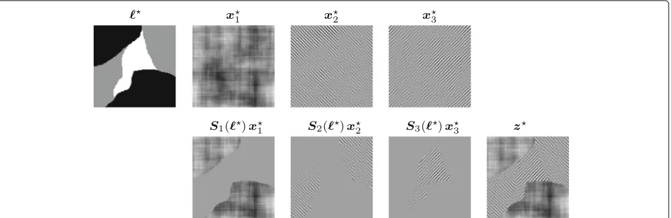
the schematic in Fig. 1. This image forming process is mathematically formalized as:
whereSk()areP×Pdiagonal binary matrices obtained
based on the labels. These matrices extract from the tex-tured imagexkthe pixels with labelkand replace the other
pixels with 0. They are zero-forcing matrices defined by:
Sk()=diag
δ(p,k),p=1,. . .P
Fig. 1Image forming process (see Eq. (4)) in a case withK=3 texture classes. Left: true label. Central panel: three imagesx1,x2andx3(top) and extracted partsS1()x1,S2()x2andS3()x3(bottom). Right: true imagez
Remark 5Let us considerIk = p|p=kthe set of sites having label k. Then, these sets for k=1,. . .K encode a repartition of the set of pixel indices, thus having the properties:
• Are disjoint, i.e.,Ik∩Il=∅, forl=k
• Cover the entire lattice, i.e.,∪kIk = {1,. . .P}
• May be empty
In terms of the extraction matrices, these properties are summarized by Kk=1Sk = IP, the identity matrix of size P.
2.4 Observation system model
Now we turn to the observation system that is modelled as a linear and invariant transform. It is accounted for through aP×Pconvolution matrix with a TbT structure
denoted by H. It becomes CbC by circulant
approxi-mation, and its eigenvalues are defined by the Fourier transfer function h◦p. Any function could be introduced
(Gaussian, Lorentzian, Airy,. . . ), and the considered one is a Laplacian:
◦
hnm=exp
−w−1(|νn| + |νm|) /2
centred in the(0, 0)frequency with widthw. This is only one of the countless models that can be used.
2.5 Noise model
The noise is considered to be additive, zero-mean, white, and Gaussian of inverse varianceγn. Based on this model,
the density of the data given the imagez and the noise parameterγn, reads:
f(y|z,γn)=(2π)−PγnP exp
−γny−Hz2
(5)
that is to say the likelihood.
2.6 Hierarchical model
Based on the variables above, the hierarchy for the model in preparation for the segmentation problem from blurred and noisy data can be established and it is graphically represented in Fig. 2. Based on the variable dependen-cies encoded in this figure, the joint distribution can be expressed:
f(y,,x1...K,γn,γ1...K,θ1...K)=f(y|γn,,x1...K)
Pr [|β]
K
k=1
f(xk|θk,γk)
f(β)f(γn) K
k=1 f(θk)
K
k=1 f(γk).
(6)
Fig. 2Hierarchical model: the round/square nodes show the estimated/given variable. Thexkare the textured images (Gaussian
density) and theθk,γkare the texture parameters.is the label set
In order to complete the probabilistic description, the next section introduces the hyperparameter densities.
2.7 Hyperparameter models
Regarding the precision parameters γk,k = 1,. . .K
and γn, it can be noticed that in the model for the
textured images xk (Eq. (2)) and for the observation y (Eq. (5)), they intervene as precision parameters in Gaussian conditional densities; hence, the Gamma den-sities Gγ;α0,β0 are conjugate forms. Furthermore, little prior information is available on these parame-ters, so uninformative Jeffreys prior are used, by setting
α0,β0→(0, 0).
Otherwise, the dependency of the likelihood w.r.t. the parameterθk is very complicated, meaning that there is no conjugate form. Moreover, the lack of prior informa-tion suggests the use of the uniform density between a minimum and a maximum value:f(θk)=Uθm
k,θMk
(θk).
When it comes toβ, a conjugate prior is not available, given the expression of the partition function Z(β). A uniform prior on an interval [ 0,B] is considered as a rea-sonable choice:f(β)=U[0,B](β)whereBis defined as the
maximum possible value ofβ.
3 Method: Bayesian formulation
3.1 Estimation
The Bayesian strategy designs an estimator based on a loss function that quantifies the discrepancy between the true value of a parameter and an estimated one. It then relies on a risk that is the mean value of the loss function, the mean being considered under the joint distribution (6) that is to say the distribution of the unknown parameters and the data. The optimal estimator is defined as the function of the data that minimizes the risk. It is naturally different for the various types of parameters and choices of loss function.
• Regarding the labels(discrete parameters), we resort to a binary loss function and the estimates are themarginal posterior maximizers.
• Regarding the continuous parametersβ,γn, theγk,
theθkand thexk, we resort to the quadratic loss
function and the estimates are theposterior means.
Remark 6A specificity of the chosen loss functions is separability, resulting in marginal estimates. It allows for relatively fast computations but with possible limi-tations regarding image quality. Alternatives could rely on non-separable loss function and non-marginal esti-mates, for instance (joint) posterior maximizer. Numerical implementation could then rely on non-guaranteed opti-mization algorithm (e.g. block iterative conditional mode) or on computationally intensive algorithm (e.g. simulated annealing).
An estimatez of the image z can be obtained based
on the estimated labelsand textured imagesxk based
on Eq. (4) as follows:
z= k
Sk()xk (7)
each extraction matrix being based on the label estimate.
3.2 Posterior
The posterior is proportional to the joint distribution (6) and is fully specified based on the formation model (4) for the imagez, the model (2) for the textured imagesxk,
This distribution summarizes all the information about the unknowns contained by the data and the prior models.
3.3 Computing—posterior conditionals
Due to the sophisticated form of the posterior, the esti-mates (marginal posterior maximizers or means) can-not be calculated; consequently, they will be numerically extracted. Stochastic samplers seem adequate and the lit-erature on the subject is abundant and varied [47–50]. More specifically, a (block) Gibbs loop is particularly appealing since it enables to split the global sophisticated problem in several far simpler sub-problems. It requires to sequentially sample each variable, under its conditional posterior. These distributions are described in the next section.
4 Algorithm: sampling aspects
Each conditional posterior can be deduced from the joint posterior (8) by picking the factors that are function of the considered parameter.
4.1 Precision parameters
Regarding the noise parameterγn and the texture scale
parametersγk, from (8), we have:
They must be sampled under Gamma densitiesG(γ;α,β) with respective parameters:
α=α0
n+P and β=βn0+ y−Hz2
for the noise parameterγnand
α=α0
k +P and β=βk0+ xk2k(θk)
for the texture parametersγk. As Gamma variables, they can be straightforwardly sampled. In addition, given the hierarchical structure (see Fig. 2), they are mutually (a posteriori) independent.
4.2 Shape texture parameters
Regarding the shape parametersθk of the textured image
PSD, the problem is made far more complicated by the intricate relation between the density, the PSD and the parameterθk; see Eqs. (2) and (3). As a consequence, the
conditional posterior has a non-standard form:
θk∼U[θm
k,θMk](θk)
p
λp(θk)exp−γkλp(θk)|x◦k,p|2
nevertheless, it can be sampled using a Metropolis-Hastings (MH) step2. Basically, it consists in drawing a proposal based on a proposition law, evaluating an accep-tance probability, and then, at random according to this probability, setting the new value as the proposal (accep-tation) or as the current value (duplication). There are numerous options in order to formulate a proposition law, and both the convergence rate and the mixing proper-ties are influenced by its adequacy to the (conditional) posterior. Thus, designing a proposition law that embeds information about the posterior will significantly enhance the performances. In this context, the directional Random Walk MH (RWMH) algorithm taking advantage of first-or second-first-order derivatives of the posterifirst-or seems rele-vant. A standard case is the Metropolis-adjusted Langevin algorithm (MALA) [51], which takes advantage of the pos-terior derivative. The preconditioned MALA [52] and the quasi-Newton proposals [53] exploit the posterior curva-ture. More advanced versions rely on the Fisher matrix (instead of the Hessian) and leads to an efficient sampler
called the Fisher-RWMH: [54] proposes a general state-ment and our previous paper [55] (see also [56]) focuses on texture parameters.
Explicitly, from the current valueθc, the algorithm
for-mulates the proposalθp:
θp=θc+
1 2ε
2I−1(θc)L(θc)+εI(θc)−1/2u
where I(θ) is the Fisher matrix, L(θ) is the log of the conditional posterior andL(θ)its gradient,εis a tuning parameter andu∼N(0,I)a standard Gaussian sample.
4.3 Potts parameter
The granularity coefficient β conditionally follows an intricate density also deduced from (8):
β∼Z(β)−1 exp
The sampling is a very difficult task first of all because the density does not have a standard form. Moreover, the major problem is thatZ(β)is intractable, so the density cannot even be evaluated for a given value ofβ.
To overcome the obstacle, the partition functionZ(β) has been precomputed on a fine grid of values forβ,
rang-ing fromβ = 0 toβ = B = 3, with a step of 0.01, for
several numbers of pixelPand numbers of classK. Details are given in Annex6. It is therefore easy to compute the cumulative density functionF(β)by standard numerical integration / interpolation. Then, it suffices to sample a uniform variableuon [0, 1] and to computeβ=F−1(u)to
obtain a desired sample. So, this step is inexpensive (since the table of values ofZ(β)is precomputed).
Remark 7Although it allows for very efficient com-putations, this approach has a limitation: Z must be precomputed for the considered number of pixel P and class K.
The procedure is identical to the one presented in our previous papers [40, 41, 57]. The reader is invited to consult [29, 42–46] for alternatives and complementary results.
4.4 Textured image
Remark 8 To improve the readability, in the following, we will use the simplified notationk=k(θk).
The textured imagexkhas a Gaussian density, deduced
from (8):
and it is easy to show that the meanμkand the covariance
−1
the extraction of the contribution of the imagexkfrom the
data. More specifically,y¯k relies on the subtraction from the observationsyof the convolution of all the parts of the imagezthat are not labelledk.
However, the practical sampling of this Gaussian den-sity is a thorny issue due to the high dimension of the variable. Usually, sampling a Gaussian density requires handling the covariance or the precision, for instance fac-torization (e.g., Cholesky), diagonalisation, or inversion, which are impossible here. This could be possible for special structures, e.g., sparse or circulant. Here,k, H
and by extensionH†H are CbC; however, the presence
of theSk breaks the circularity:k is not diagonalizable
by FFT and, consequently, the sampling ofxk cannot be
performed efficiently in the Fourier domain.
Nevertheless, the literature accounts for alternatives based on the strong links between matrix factorization, diagonalization, inversion, linear system and optimiza-tion of quadratic criteria [58–62]. We resort here to our previous work [61] (see also [63]) based on a perturbation-optimization (PO) principle: adequate stochastic pertur-bation of a quadratic criterion and optimization of the perturbed criterion. It is shown that the criterion opti-mizer is a sample of the target density. It is applicable if the precision matrix and the mean can be written as a sum of the form:
By identification, withN=2: ⎧
The perturbation phase of this algorithm consists in draw-ing the followdraw-ing Gaussian samples:
ξ1∼N(m1,C1) and ξ2∼N(m2,C2)
The cost of these sampling is not prohibitive:ξ1is a real-ization of a white noise andξ2is a realization of the prior model forxkand it is computed by FFT.
4.4.2 Optimization
In order to obtain a sample of the imagexk, the following criterion must be optimized w.r.t.x:
Jk(x)=γnξ1−HSkx2+γkξ2−x 2
k .
For notational convenience, let us rewrite:
Jk(x) = x†Qkx−2x†qk+Jk(0)
where the matrixQk = γnS†kH†HSk +γkk is half the
Hessian (and the precision matrix) and the vectorqk = γnS†kH†ξ1+γk−k1ξ2is the opposite of the gradient at the
origin. The gradient atxitself is:gk =2(Qkx−qk).
Theoretically, there is no constraint on the optimization technique to be used and the literature on the subject is abundant [64–66]. We have only considered algorithms that are guaranteed to converge (to the unique minimizer) and among them the basic directions:
• Gradient descent,
• Conjugate gradient descent.
We have first used the conjugate gradient direction, since it is more efficient especially for a high-dimension problem and a quadratic criterion. However, we have experienced convergence difficulties, making the overall algorithm very slow. In practice, the step length at each iteration was extremely small, probably due to condi-tioning issues. Consequently, the differences between the iterates were almost insignificant. The solution relies on a preconditioner. It has been defined as a CbC approxima-tion of the inverse Hessian ofJk:
k =
γnH†H+γkk
−1
/2 (10)
obtained by eliminating theSk matrix fromQk and
cho-sen for computational efficiency. It is used for both of the aforementioned directions:
• Preconditioned gradient descent,
• Preconditioned conjugate gradient descent.
In this context, the two methods have yielded similar results, and finally, we have focused on thepreconditioned gradient.
The second ingredient that is necessary is the step lengthsin the considered direction, at each iteration. Here again, a variety of strategies is available. We have used an
optimal stepthat is explicitly given:
s= gk
• The vectorqkwrites:
and thus efficiently computed through a FFT and zero-forcing (ZF).
and thus also efficiently computed through a series of FFT and ZF.
• Regardingkgk, since the matrixkis CbC, the product can also be efficiently computed by FFT.
The zero-forcing process is achieved in the spatial domain (it amounts to setting to zero some pixels of images), while the costly products by matrices are performed in the Fourier domain (all of them by FFT).
4.5 Labels
The label set has a multidimensional categorical distribu-tion:
and it is a non-separable and non-standard form, so its sampling is not an easy task. A solution is to sample thep one by one conditionally on the others and on the rest of the variables, in a Gibbs scheme.
To this end, let us introduce the notation zpk for the image with all its pixels identical to z except for pixel
p. The pixel pin zpk is the pixelpfrom xk. Let us note Ep,k = y−Hzpk2. This error quantifies the discrepancy
between the data and the classkregarding pixelp. Sampling a labelp0 requires its conditional probability. A precise analysis of the conditional distribution forp0 yields: multiplicative constant, which can be determined know-ing that the probabilities sum to 1.
To compute these probabilities, we must evaluate the two terms of the argument of the exponential function, at pixelp0. The first term is the contribution of the prior
and it can be easily computed for eachkby counting the neighbours of pixelp0having the labelk. Let us now focus
on the second term, Ep,k. To write this term in a more
convenient form, we introduce:
• A vector1p∈RP: itsp-th entry is 1 and the other is 0. • A quantityp,k ∈Rthat records the difference
between thep-th pixel of the imagezand the one of imagexk:p,k=1†p(z−xk). Consequently, its value is not required in the sampling process and it can be included in a multiplicative factor.
2. The term1†pH†H1p= H1p2does not depend on
p due to the CbC form of theHmatrix. Moreover, this norm only needs to be computed once for all, since theHmatrix does not change throughout the iterations. In fact, this norm amounts to the sum
q| ◦ hq|2.
3. Finally, in the third term1†pH†y¯, the productH†y¯is a
convolution efficiently computable by FFT and the product with1†pselects the pixelp. Under this form,
the computation would not be efficient sinceH†y¯
should be recomputed at each iteration. A far better alternative is to updateH†y¯after updating each label. 5 Results and discussion
The problem of texture segmentation has a considerable degree of difficulty, especially in the present case, where (i) the data are affected by blur and noise, (ii) the texture parameters are unknown and (iii) the granularity coeffi-cient, the signal and the noise levels are also unknown. The previous sections provide a detailed description of our method, and this section presents numerical results, as follows.
1. First, implementation and practical considerations are described.
2. A study is then given for different image topologies in various combinations of blur and noise to assess the method versatility and identify the limitations. 3. Moreover, a posterior statistics analysis is given in
5.1 Implementation and practical considerations
The method has been implemented3 as shown in
Algorithm 1. Under different scenarios, the algorithm has been run several times from identical and different
Algorithm 1:Deconvolution-Segmentation of Textures
Input : Datay, texture numberK,impulse response
Output: Samples for labels(t), texturesx(kt),
% Count label occurrences and update segmentation
LabelOcc(p,p)=LabelOcc(p,p)+1,p=1,. . .P; =MaxOccurrenceLabel(LabelOcc);
% Update parameters;
xk =UpdateAverage
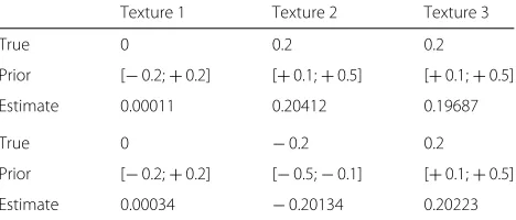
Table 1The horizontal and vertical frequenciesν0xandνy0are respectively given in the top and the bottom part of the table. For each parameter, it gives the true value, the prior interval and the estimated values. They are clearly very closed to the true ones
Texture 1 Texture 2 Texture 3
True 0 0.2 0.2
Prior [−0.2;+0.2] [+0.1;+0.5] [+0.1;+0.5]
Estimate 0.00011 0.20412 0.19687
True 0 −0.2 0.2
Prior [−0.2;+0.2] [−0.5;−0.1] [+0.1;+0.5]
Estimate 0.00034 −0.20134 0.20223
initializations, and it has shown consistent qualitative and quantitative behaviours. It has lead us to a series of practical considerations.
• The label set is initialized by a realization of a white noise with uniform probability in{1,. . .K}. Our tests have shown a faster convergence as compared to other initialization (e.g. constant label field). • An important practical point is the initialization of
the texture parametersθk. Each frequency is set to
the maximizer of the periodogram of the observed imageyover its prior interval.
• The preconditioned gradient and the preconditioned conjugate gradient directions have similar
performances. Contrary, the non preconditioned versions are very slow.
• Stopping rule: the algorithm stops when the
difference between successive updates of the imagez
(see Eq. (7) and last line of Algorithm 1) becomes smaller than a given thresholds. Practically, we set
s=10−3, the algorithm iterates usually about two hundred times and it takes about 4 min for a 256×256image.
5.2 Evaluation of the method
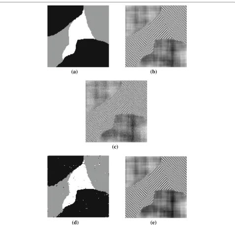
The first example is given in Fig.4. It consists in a sim-ple image topology containingK = 3 classes of texture. The true values of the frequency parameters of the tex-tured images are given in Table1. The value of the spectral
width is ux = uy = 0.005 for all the textures (and
it is assumed to be known). These values produce two oriented textures and a low-frequency noise shown in Fig.4(and already given in Fig.1). The observation
sce-nario is with w = 1/2 (full width at half maximum
is about 0.5) and γn = 10 (signal to noise ratio is
about 5 dB).
For an illustrative plot, the algorithm has been iter-ated arbitrarily 100 times and Fig.3shows the simulated chains for the granularity coefficientβ and for the noise parameter γn. It shows that the distributions are stable
after aboutT =50 iterations (burn-in period). The firstT
samples are then discarded. From the remaining samples, the decisions for the labels are computed as the empiri-cal marginal posterior maximizers and the estimations for the other parameters are computed as empirical posterior averages.
The algorithm produces a label configuration (Fig.4d) very similar to the true one (Fig. 4a), with only 0.90%
of mislabelled pixels, despite the degradation of the image.
Remark 9The method is region-based, meaning that it provides closed contours, unlike a part of the existing works in texture segmentation.
Moreover, the texture parameters estimation error is small, less than 10−2, as mentioned in Table1. The full textured imagesxk are also accurately estimated, having
the same characteristics as the original textured images. The blur and the noise are reduced in the resulting image (Fig.4e) with respect to the data (Fig.4c), and it strongly resembles the original image (Fig.4b).
5.2.1 Label analysis: error and probability of error
One of the main advantages of probabilistic approaches is that they not only provide estimates for the unknowns, but also coherent uncertainties associated to these estimates. Figure5illustrates our analysis on the label estimates and their probability.
Figure5a gives the empirical marginal probabilities for
the three values of the labelp = 1,p = 2 andp = 3
for each pixels p = 1,. . .P. Figure5b gives the proba-bilities of the selected labels (the one with the maximum probability). This maximum probability can have various values: a small value indicates a less reliable decision for the label. These probabilities are small (black or grey) at
certain locations in the image Fig. 5b, and it is safe to assume that at these locations, there is a smaller chance of selecting a correct label.
This analysis can naturally be done even without the knowledge of the true labels. In order to verify if indeed we are more prone to error in the area with small posterior probability, we have compared the selected label configu-rationto the true one. We can immediately notice in Fig.5c that all of the mislabelled pixels are in fact posi-tioned in the areas of weaker probability, shown in Fig.5b. This reinforces our statement concerning the utility of the probabilistic approach, due to its ability to anticipate errors.
5.2.2 Other image topologies, blur and noise
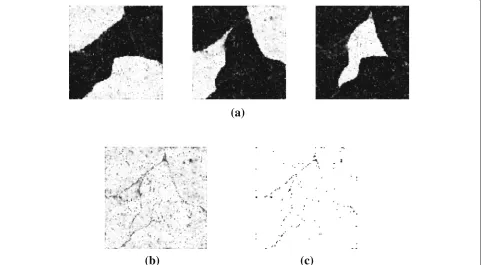
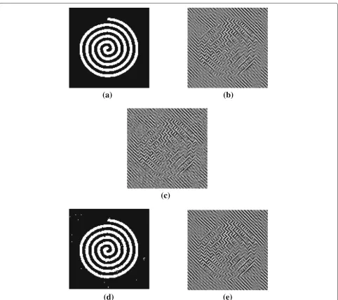
In the case of the second image topology, given in Fig.6, although the number of textures is reduced (K = 2), the task is more difficult due to the shape of the regions: the presence of a relatively thin, continuous structure makes the label decision hard. In addition, only a small patch of the texture associated with the “white” class is present and that complicates the texture parameter estimation. How-ever, the results shown in Fig.6are remarkably correct, for both label and image. We only have 0.64% of mislabelled pixels.
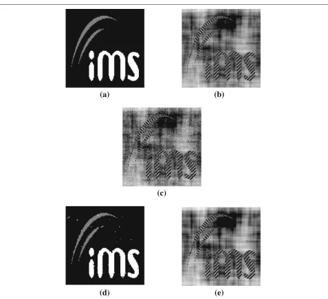
Our third example is given in Fig. 7. Here again, the shape of some of the regions are relatively thin making the label decision hard and only a small patches of the
Fig. 6Segmentation and reconstructed images (Example 2).aTrue labels∗.bTrue imagez∗.cDatay.dEstimated labelsˆ.eEstimated imagezˆ
second texture class is observed making texture parameter estimation difficult. Figure7illustrates the method per-formances in a weaker convolution casew=2 and higher noise levelγn=5. The method performs very well in this
case, the estimated label field being very close to the true labels (only 0.70% of miss-labelled pixels).
6 Conclusion and perspectives
The paper presents our method for joint deconvolution and segmentation, dedicated to textured images, with an emphasis on oriented structures. This is a very dif-ficult task due to the large amount of unknowns and their complicated dependencies. The formulation of the
problem itself has demanded a careful consideration in order to design the best manner to accurately account for the hierarchical dependencies. In this context, the most adapted choice was to modelK full imagesxk
cor-responding to each class, rather than directly model the compound image zitself. This has allowed us to obtain an expression for the joint probability distribution in a relatively convenient form.
Fig. 7Segmentation and reconstructed images (Example 3).aTrue labels∗.bTrue imagez∗.cDatay.dEstimated labelsˆ.eEstimated imagezˆ
intricate nature of the posterior distribution does not allow for an analytical expression for either the deci-sions or the estimates. A numerical approach is then used to explore the posterior, and the samples are subsequently used in computing them. The numerical scheme is guaranteed to converge: samples are asymptot-ically drawn under the posterior and empirical approx-imation converges towards the optimal decisions and estimates.
Nevertheless, the sampling process for the full set of variables has also proved to be challenging and has required advanced sampling approaches to overcome the impasses. We resort to a Gibbs sampler in order to split
the original problem for the full set of variables in several smaller problems for subsets of variables.
(i) One of the steps requires the sampling of a Gaussian density in large dimension and we resort to recent developments on Perturbation-Optimization. (ii) The method includes the sampling of the granularity
coefficient: it is itself a thorny question, hardly ever tackled. The proposed approach relies on the inverse cumulative density function and takes advantage of our precomputations of the partition function. (iii) Regarding the texture parameters, the algorithm
Metropolis-Hastings step within the Gibbs loop.
The proposed methodological aspects are original and have contributed to developing an approach that is both theoretically sound and practically efficient for the problem.
The previous section has presented the results of a series of numerical assessments performed on various convolu-tion and noise condiconvolu-tions, for different image topologies. These results have shown that the method is able to accurately segment the image, provide a good estimation for the texture parameters as well as the hyperparameters and thus accurately restore the original image.
From a theoretical and modelling standpoint, the study leads us to several future developments.
• A future contribution is the use of a non-Gaussian model for the constituent textures, possibly based on latent variables and conditional Gaussian models [67]. This would add an extra layer of complexity to the model and to the sampling stage.
• The second future development aims at performing a myopic deconvolution [56,68], i.e., considering thatw, the width of the convolution filter, is
unknown and estimating it along with the rest of the parameters.
• Thirdly, the problem of missing data (inpainting) will also be addressed. An extension of the present work to solve this problem would require to include a truncation matrix, sayT, and substituteHbyTH
in (5).
• The fourth future contribution will deal with the problem of model selection, especially to choose the number of classes [69] (see also our previous works [70–72]). The difficulty would regard the
computation of the evidences of the models.
The study also opens up new perspectives from a numerical standpoint, notably in order to reduce compu-tation time.
• A future contribution will resort to the
Swendsen-Wang algorithm in order to improve the sampling step of the label field [73] (see also [74]). • The second future development in order to reduce
computation time could rely on variational Bayes approaches [30,32,75] (see also [76,77]). • Thirdly, the problem of fast sampling will also be
addressed through the abundant literature as already mentioned [47–54] and more recently [78].
As it can be seen from this brief listing of the per-spectives, the work on this topic is far from being over. Nevertheless, even in its current form, the method
presented in this paper addresses a problem that had not been tackled so far (deconvolution-segmentation of textured images including hyperparameter and texture parameter estimation), while achieving very satisfactory results.
Endnotes
1Except for the Ising field (K=2), see [79], also [80,81].
2A unique step is used, in order to design a valid algorithm.
3The algorithm is implemented within the computing
environment Matlab on a standard PC with a 3 GHz CPU and 64 GB of RAM.
Appendix A: Potts partition
For the sake of self-containedness, we describe here the pre-computation of the partition function already given in our previous paper [40]. It is based on known properties [38,39] for the partition function of the exponential family distributions.
Let us noteσ() = p∼qδ(p;q)the number of pair of adjacent pixels with identical label. The partitionZ(β) normalizes the probability distribution (1), so it writes:
Z(β)=exp [βσ()]
where the summation runs over all the configurations of the field ∈ {1, ...K}P. Numerically, it is a colossal summation over the KP possible configurations and the exhaustive exploration of these configurations is impossi-ble (except for minuscule images). The derivation w.r.t.β straightforwardly yields:
Z(β)=
σ()exp [βσ()]
then dividing byZ(β)we have
Z(β)
Z(β) =
σ()Z(β)
−1exp [βσ()] .
The left-hand side reads as the derivative of the log-partitionZ(β)¯ = logZ(β)and the right-hand side reads as an expectation:
¯
Z(β)=
σ()Pr [|β]=E [σ(L)] .
Consequently, the derivative of the log-partition is an expectation. It can be approximated by an empirical average:
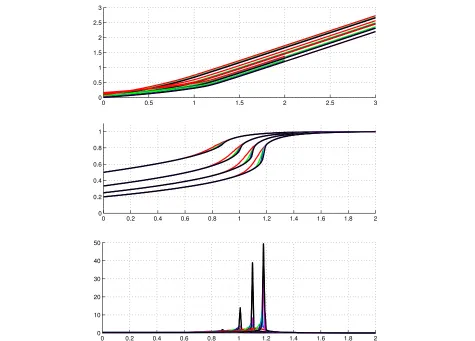
Fig. 8From to to bottom: Log-partitionZ¯(β), its first and second derivatives as a function ofβ(fromβ=0 toβ=3) for various sizes of image (P=64, 128, 256, 512)and number of class(K=2, 3, 4, 5)
Abbreviations
∼: Neighbor relation between pixels;β: Granularity coefficient (Potts field);K: Number of texture classes;: Unobserved (hidden) labels;NN:
{0, 1,. . .,N−1};θk: Texture parameters;P: Number of pixels;Rk,k: Texture covariance and precision structure;xk: Unobserved (hidden) textured images;
y: Observed image;γk,γn: Texture and noise levels;z: Unobserved (hidden)
image;Z: Partition function (Potts field);δ(·,·): Kronecker function; CbC: Circulant-block-circulant; MALA: Metropolis adjusted Langevin algorithm; MCMC: Monte Carlo Markov chain; MH: Metropolis-hastings; PSD: Power spectral density; RWMH: Random walk metropolis-hastings; TbT: Toeplitz-block-toeplitz; w.r.t.: With respect to; ZF: Zero-forcing
Acknowledgements
Not applicable.
Funding
Not applicable.
Availability of data and materials
Please contact the author for data requests.
Authors’ contributions
Both authors jointly developed the work presented in this paper. Both authors read and approved the final manuscript.
Competing interests
The authors declare that they have no competing interests.
Publisher’s Note
Springer Nature remains neutral with regard to jurisdictional claims in published maps and institutional affiliations.
Received: 26 November 2016 Accepted: 10 December 2018
References
1. M. Petrou, P. Garcia-Sevilla,Dealing with Texture. (Wiley, Chichester, England, 2006)
2. G. L. Gimel’farb,Image Textures and Gibbs Random Fields. (Kluwer Academic Publishers, 1999)
3. J. P. Da Costa, F. Michelet, C. Germain, O. Lavialle, G. Grenier, Delineation of vine parcels by segmentation of high resolution remote sensed images. Precision Agric.8, 95–110 (2007)
4. J. P. Da Costa, F. Galland, A. Roueff, C. Germain, Unsupervised segmentation based on Von Mises circular distributions for orientation estimation in textured images. JElectron Imaging.21(2) (2012) 5. J. C. Russ,The Image Processing Handbook (Seventh Edition). (CRC Press,
2015)
6. J. Zhang, J. Zheng, J. Cai, inIEEEConference on Computer Vision and Pattern Recognition. A diffusion approach to seeded image segmentation, (2010), pp. 2125–2132
8. S. Alpert, M. Galun, A. Brandt, R. Basri, Image Segmentation by Probabilistic Bottom-Up Aggregation and Cue Integration. IEEE Trans. Pattern. Anal. Mach. Intell.34(2), 315–327 (2012)
9. T. F. Chan, P. Mulet, On the convergence of the lagged diffusivity fixed point method in total variation image restoration. SIAM Numer J. Anal.
36(2), 354–367 (1999)
10. J. Malik, S. Belongie, T. Leung, J. Shi, Contour and Texture Analysis for Image Segmentation. Int. Comput J. Vis.43, 7–27 (2001)
11. L. Grady, Random Walks for Image Segmentation. IEEE Trans. Pattern. Anal. Mach. Intell.28(11), 1768–1783 (2006)
12. A. K. Sinop, L. Grady, inIEEE International Conference on Computer Vision. ASeeded Image Segmentation Framework Unifying Graph Cuts And Random Walker Which Yields ANew Algorithm, (2007), pp. 1–8 13. M. Tuceryan, Moment-based texture segmentation. Pattern Recogn. Lett.
15(7), 659–668 (1994)
14. S. Arivazhagan, L. Ganesan, Texture segmentation using wavelet transform. Pattern. Recogn. Lett.24, 3197–3203 (2003)
15. L. Wolf, X. Huang, I. Martin, D. Metaxas, inIn European Conference on Computer Vision. Patch-based texture edges and segmentation, (2006) 16. A. Lillo, G. Motta, J. A. Storer, inPattern Recognition and Image Analysis. vol.
4477 of Lecture Notes in Computer Science, ed. by J. Martí, J. M. Benedí, A. M. Mendonça, and J. Serrat. Supervised Segmentation Based on Texture Signatures Extracted in the Frequency Domain (Springer Berlin Heidelberg, 2007), pp. 89–96
17. H. Mobahi, S. Rao, A. Y. Yang, S. S. Sastry, Y. Ma, Segmentation of Natural Images by Texture and Boundary Compression. Int. Comput, J. Vis.95(1), 86–98 (2011)
18. M. Galun, E. Sharon, R. Basri, A. Brandt, inIEEEInternational Conference on Computer Vision. vol. 1. Texture segmentation by multiscale aggregation of filter responses and shape elements, (2003), pp. 716–723
19. X. Liu, D. Wang, Image and Texture Segmentation Using Local Spectral Histograms. IEEE Trans. Image Process.15(10), 3066–3077 (2006) 20. S. Todorovic, N. Ahuja, inIEEE International Conference on Computer Vision.
Texel-based texture segmentation, (2009), pp. 841–848 21. D. Geman, S. Geman, C. Graffigne, P. Dong, Boundary Detection by
Constrained Optimization. IEEE Trans. Pattern. Anal. Mach. Intell.12(7), 609–628 (1990)
22. Z. Tu, S. C. Zhu, H. Y. Shum, inIEEE International Conference on Computer Vision. vol. 2. Image segmentation by data driven Markov chain Monte Carlo, (2001), pp. 131–138
23. H. Deng, D. A. Clausi, Unsupervised image segmentation using a simple MRF model with a new implementation scheme. Pattern. Recognit.
37(12), 2323–2335 (2004)
24. P. F. Felzenszwalb, D. P. Huttenlocher, Efficient Graph-Based Image Segmentation. Int. Comput, J. Vis.59(2), 167–181 (2004) 25. Y. Boykov, G. Funka-Lea, Graph cuts and efficient ND image
segmentation. Int. Comput, J. Vis.70(2), 109–131 (2006)
26. G. Celeux, F. Forbes, N. Peyrard,EM-based image segmentation using Potts models with external field. (INRIA, 2002)
27. R. Morris, X. Descombes, J. Zerubia,Fully Bayesian image segmentation - an engineering perspective. (INRIA, Sophia Antipolis France, 1996). 3017 28. A. Barbu, S. C. Zhu, Generalizing Swendsen-Wang to sampling arbitrary
posterior probabilities. IEEE Trans. Pattern. Anal. Mach. Intell.27(8), 1239–1253 (2005)
29. M. Pereyra, N. Dobigeon, H. Batatia, J. Y. Tourneret, Estimating the Granularity Coefficient of a Potts-Markov Random Field within a Markov Chain Monte Carlo Algorithm. IEEE Trans. Image Process.22(6), 2385–2397 (2013)
30. O. Féron, B. Duchêne, A. Mohammad-Djafari, Microwave imaging of inhomogeneous objects made of a finite number of dielectric and conductive materials from experimental data. Inverse Problems.21(6), 95–115 (2005)
31. M. Mignotte, A Segmentation-Based Regularization Term for Image Deconvolution. IEEE Trans. Image Process.15(7), 1973–1984 (2006) 32. H. Ayasso, A. Mohammad-Djafari, Joint NDT Image Restoration and
Segmentation Using Gauss-Markov-Potts prior Models and Variational Bayesian Computation. IEEE Trans. Image Process.19(9), 2265–2277 (2010) 33. O. Eches, N. Dobigeon, J. Y. Tourneret, Enhancing hyperspectral image
unmixing with spatial correlations. IEEE Trans. Geosci. Remote Sens.
49(11), 4239–4247 (2011)
34. M. Pereyra, N. Dobigeon, H. Batatia, J. Y. Tourneret, Segmentation of skin lesions in 2D and 3D ultrasound images using a spatially coherent generalized Rayleigh mixture model. IEEE Trans. Med. Imaging.31(8), 1509–1520 (2012)
35. O. Eches, J. A. Benediktsson, N. Dobigeon, J. Y. Tourneret, Adaptive Markov random fields for joint unmixing and segmentation of hyperspectral image. IEEE Trans. Image Process.22(1), 5–16 (2013) 36. Y. Altmann, N. Dobigeon, S. McLaughlin, J. Y. Tourneret, Residual
component analysis of hyperspectral images - Application to joint nonlinear unmixing and nonlinearity detection. IEEE Trans. Image Process.
23(5), 2148–2158 (2014)
37. M. Storath, A. Weinmann, J. Frikel, M. Unser, Joint image reconstruction and segmentation using the Potts model. Inverse Probl. 31 (2015) 38. G. Winkler,Image Analysis, Random Fields and Markov Chain Monte Carlo
Methods. (Springer Verlag, Berlin, Germany, 2003)
39. D. MacKay,Information Theory, Inference, and Learning Algorithms. (Cambridge University Press, 2008)
40. R. Rosu, J. F. Giovannelli, A. Giremus, C. Vacar, inProceedings of the International Conference on Acoustic, Speech and Signal Processing. Potts model parameter estimation in Bayesian segmentation of piecewise constant images, (Brisbane, Australia, 2015)
41. J. F. Giovannelli, A. Barbos, inProceedings of the International Conference on Statistical Signal Processing. Unsupervised segmentation of piecewise constant images from incomplete, distorted and noisy data, (Palma de Majorque, Spain, 2016)
42. L. Risser, T. Vincent, P. Ciuciu, J. Idier,Application to within-subject fMRI data analysis, (London England, 2009)
43. N. Friel, A. N. Pettitt, R. Reeves, E. Wit, Bayesian inference in hidden Markov random fields for binary data defined on large lattices. Comput, J. Graph. Stat.18, 243–261 (2009)
44. J. Moller, A. N. Pettitt, R. Reeves, K. K. Berthelsen, An efficient Markov chain Monte Carlo method for distributions with untractable normalising constants. Biometrika.93(2), 451–458 (2006)
45. A. N. Pettitt, N. Friel, R. Reeves, Efficient calculation of the normalizing constant of the autologistic and related models on the cylinder and lattice. J. Royal Stat. Soc. B.65(1), 235–246 (2003)
46. R. Reeves, A. N. Pettitt, Efficient recursions for general factorisable models. Biometrika.91(3), 751–757 (2004)
47. J. M. Marin, C. P. Robert,Bayesian Core. APractical Approach to
Computational Bayesian Statistics. Texts in statistics. (Springer, Paris, France, 2007)
48. J. Albert,Bayesian Computation With R. (Springer-Verlag New York Inc., New York, 2009)
49. C. P. Robert, G. Casella,Monte-Carlo Statistical Methods. Springer Texts in Statistics. (Springer, New York, 2004)
50. D. Gamerman, H. F. Lopes,Markov Chain Monte Carlo: stochastic simulation for Bayesian inference. 2nd ed.(Chapman & Hall/CRC, Boca USA Raton, 2006)
51. G. O. Roberts, R. L. Tweedie, Exponential Convergence of Langevin Distributions and Their Discrete Approximations. Bernoulli.2(4), 341–363 (1996)
52. G. Roberts, O. Stramer, Langevin Diffusions and Metropolis-Hastings Algorithms. Methodol. Comput. Appl. Probab.4, 337–358 (2003) 53. Y. Qi, T. P. Minka, inFirst Cape Cod Workshop on Monte Carlo Methods.
Hessian-based Markov Chain Monte-Carlo Algorithms (Cape Cod, Massachusetts, USA, 2002)
54. M. Girolami, B. Calderhead, Riemannian manifold Hamiltonian Monte Carlo (with discussion). J. Royal Stat. Soc. B.73, 123–214 (2011) 55. C. Vacar, J. F. Giovannelli, Y. Berthoumieu, inProceedings of the
International Conference on Acoustic, Speech and Signal Processing. Langevin and Hessian with Fisher approximation stochastic sampling for parameter estimation of structured covariance, (Prague, Czech Republic, 2011), pp. 3964–3967
56. C. Vacar, J. F. Giovannelli, Y. Berthoumieu, Bayesian texture and instrument parameter estimation from blurred and noisy images using MCMC. IEEE Signal Process. Lett.21(6), 707–711 (2014)
57. J. F. Giovannelli, C. Vacar, inEUSIPCO. Deconvolution-Segmentation for Textured Images, (Kos, Greece, 2017)
59. G. Papandreou, A. Yuille, inProc. Int. Conf. on Neural Information Processing Systems (NIPS). Gaussian Sampling by Local Perturbations, (Vancouver, Canada, 2010), pp. 1858–1866
60. A. Parker, C. Fox, Sampling Gaussian Distributions in Krylov Spaces with ConjugateGradients. SIAM J. Sci. Comput.34(3) (2012)
61. F. Orieux, O. Féron, J. F. Giovannelli, Sampling high-dimensional Gaussian fields for general linear inverse problem. IEEE Signal Process. Lett.19(5), 251–254 (2012)
62. A. Barbos, F. Caron, J. F. Giovannelli, A. Doucet. booktitle=NIPS-2017. Clone MCMC: Parallel High-Dimensional Gaussian Gibbs Sampling, (Long Beach, USA, 2017)
63. C. Gilavert, S. Moussaoui et, J. Idier, Efficient Gaussian sampling for solving large-scale inverse problems using MCMC. IEEE Trans Signal Processing.
63(1), 70–80 (2015)
64. D. P. Bertsekas,Nonlinear programming. 2nd ed.(Belmont,MAUSA: Athena Scientific, 1999)
65. J. Nocedal, S. J. Wright,Numerical Optimization. Series in Operations Research. (Springer Verlag, New York, 2008)
66. S. Boyd, N. Parikh, E. Chu, B. Peleato, J. Eckstein,Distributed Optimization and Statistical Learning via the Alternating Direction Method of Multipliers. vol. 3 of Foundations and Trends in Machine Learning. (USA MA Now Publishers Inc, Hanover, 2011)
67. C. Vacar, J. F. Giovannelli, A. M. Roman, inProceedings of the International Conference on Image Processing. vol. 19. Bayesian texture model selection by harmonic mean, (Orlando, 2012), p. 5
68. F. Orieux, J. F. Giovannelli, T. Rodet, Bayesian estimation of regularization and point spread function parameters for Wiener–Hunt deconvolution. J. Opt. Soc. Am.27(7), 1593–1607 (2010)
69. T. Ando,Bayesian model selection and statistical modeling. (Chapman & Hall/CRC, Boca USA Raton, 2010)
70. J. F. Giovannelli, A. Giremus, inProceedings of the International Conference on Statistical Signal Processing (special session). Bayesian noise model selection and system identification based on approximation of the evidence, (Gold Coast, Australia, 2014)
71. A. Barbos, A. Giremus, J. F. Giovannelli, inActes du 25ecolloque GRETSI. Bayesian noise model selection and system identification using Chib approximation based on the Metropolis-Hastings sampler, (Lyon, France, 2015)
72. C. Vacar, J. F. Giovannelli, Y. Berthoumieu, Bayesian Texture Classification From Indirect Observations Using Fast Sampling. IEEE Trans. Signal Process.64(1), 146–159 (2016)
73. D. M. Higdon, Auxiliary Variable Methods for Markov Chain Monte Carlo with Applications. J. Am. Stat. Assoc.93(442), 585–595 (2012) 74. J. Sodjo, A. Giremus, N. Dobigeon, J. F. Giovannelli, inProceedings of the
International Conference on Acoustic, Speech and Signal Processing. A generalized Swendsen-Wang algorithm for Bayesian nonparametric joint segmentation of multiple images, (New Orleans, USA, 2017)
75. V. Smidl, A. Quinn,The variational Bayes Method in Signal Processing. (Springer, 2006)
76. W. Fan, N. Bouguila, D. Ziou, Variational learning for finite Dirichlet mixture models and applications. IEEE Trans. Neural Netw. Learn. Syst.3(5), 762–774 (2012)
77. B. Ait-El-Fquih, J. F. Giovannelli, N. Paul, A. Girard, I. Hoteit, inProceedings of the International Conference on Statistical Signal Processing. A variational Bayesian estimation scheme for parameteric point-like pollution source of groundwater layers, (Freibourg, Germany, 2018)
78. L. Martino, J. Read, D. Luengo, Independent Doubly Adaptive Rejection Metropolis Sampling Within Gibbs Sampling.63(12), 3123–3138 (2015) 79. L. Onsager, ATwo-Dimensional Model with an Order-Disorder Transition.
Phys Rev.65(3 & 4), 117–149 (1944)
80. J. F. Giovannelli, inProceedings of the International Conference on Image Processing. Estimation of the Ising field parameter thanks to the exact partition function, (Hong-Kong, 2010), pp. 1441–1444