R E S E A R C H
Open Access
Multiple particle filtering for tracking
wireless agents via Monte Carlo likelihood
approximation
Stephan Schlupkothen
*and Gerd Ascheid
Abstract
The localization of multiple wireless agents via, for example, distance and/or bearing measurements is challenging, particularly if relying on beacon-to-agent measurements alone is insufficient to guarantee accurate localization. In these cases, agent-to-agent measurements also need to be considered to improve the localization quality. In the context of particle filtering, the computational complexity of tracking many wireless agents is high when relying on conventional schemes. This is because in such schemes, all agents’ states are estimated simultaneously using a single filter. To overcome this problem, the concept of multiple particle filtering (MPF), in which an individual filter is used for each agent, has been proposed in the literature. However, due to the necessity of considering agent-to-agent measurements, additional effort is required to derive information on each individual filter from the available
likelihoods. This is necessary because the distance and bearing measurements naturally depend on the states of two agents, which, in MPF, are estimated by two separate filters. Because the required likelihood cannot be analytically derived in general, an approximation is needed. To this end, this work extends current state-of-the-art likelihood approximation techniques based on Gaussian approximation under the assumption that the number of agents to be tracked is fixed and known. Moreover, a novel likelihood approximation method is proposed that enables efficient and accurate tracking. The simulations show that the proposed method achieves up to 22% higher accuracy with the same computational complexity as that of existing methods. Thus, efficient and accurate tracking of wireless agents is achieved.
Keywords: Wireless sensor networks, Localization, Tracking, Particle filtering, Multiple particle filtering
1 Introduction
Technological advances have opened the door for a broad variety of applications of mobile agents such as robots, drones, and sensory agents, ranging from surveillance and delivery tasks to aerial and underwater exploration. In many of these applications, accurate localization of the agents is essential for successful task completion. How-ever, such localization often cannot be achieved using satellite-based systems such as GPS. Instead, in many cases, a set of local beacons1 is used, which facilitate range- and/or bearing-based localization.
*Correspondence:[email protected]
Chair for Integrated Signal Processing Systems, RWTH Aachen University, Templergraben 55, 52062 Aachen, Germany
1Beacons are stationary at positions that are known a priori.
However, in many scenarios, access to beacons is limited. This may be because their placement is costly or because good beacon locations cannot be determined a priori. Examples of such scenarios include those involv-ing underwater robots, rescue robots operatinvolv-ing in cases of disasters such as earthquakes, and the exploration of subterranean fluid-carrying structures and pipes [1,2]. In particular, the inspection of pipeline systems, e.g., pre-dictive maintenance, is an emerging application of minia-ture wireless agents. This approach promises to make obsolete the bulky robots that are currently used, which require maintenance shutdowns and thus result in pro-duction downtimes. For many of these pipeline systems, the placement of beacons would be extremely costly. In all these application cases, this beacon access limitation can be overcome through the use of numerous cooperating agents conducting range and/or bearing measurements
between pairs of agents. In such application cases, on which this paper focuses henceforth, the number of agents to be tracked is fixed and known a priori. Moreover, due to size constraints imposed on the agents and correspond-ing energy limitations, offline processcorrespond-ing of the agents’ readings, including the localization, is considered in this work. Access to the agents’ readings is, thus, only possible after the agents have been extracted from their operation domain.
Because many agents are needed to accomplish these tasks, computationally efficient methods are needed for localization. Classical (single) particle filters (PFs), for example, suffer from the “curse of dimensionality”, i.e., the fact that an exponentially increasing number of particles is required to accurately capture the posterior distribution as more agents need to be tracked [3]. This is because the dimensionality of the state space grows in proportion to the number of agents. To this end, the concept of multi-ple particle filtering (MPF), in which one particle filter is employed for each agent individually, has been proposed. However, in scenarios with limited access to beacons, such a localization process relies in large part on mea-surements between agents (agent-to-agent meamea-surements (AAMs)) rather than measurements between agents and beacons (beacon-to-agent measurements). This results in a nonseparable likelihood p(yi,k|xi,k,xj,k) because each measurement depends on two filters (the filter for agent i’s statexi,kat time stepkand the filter for agentj’s state xj,k at time step k), whereas the solution to the local-ization problem requires a likelihood for each individual filter,p(yi,k|xi,k)andp(yj,k|xj,k). Here,xi,k,yi,kdenote the state vector and measurements of agentiat timestep k, respectively.
To address this issue, a new approximation of the sought likelihood is proposed that enables higher tracking accu-racy with lower computational complexity compared with what can be achieved using the existing methods in the literature.
1.1 Related works
The literature is rich in PF-based localization algorithms; however, these algorithms are mainly used to track single or non-interacting2 agents or targets [4–7]. To mitigate the enormous computational complexity that is associated with tracking many wireless agents, the concept of mul-tiple particle filtering has been proposed. The problem of obtaining likelihood information for each individual filter based on a nonseparable likelihood was first dis-cussed in [8]. The authors proposed a technique based on the replacement of the dependency onxj,kwith a depen-dency on an estimate of agentj’s predicted state,xˆj,k =
2Interaction here refers to the presence of agent-to-agent measurement.
L
the corresponding particles and their weights from agent j’s filter. This method is called point estimate approxi-mation (PE) throughout the remainder of this manuscript because it employs the point estimatesxˆj,k.
After a series of additional papers on this topic by the same authors [9–13], in [14], the authors proposed an improved version based on an approximation of the mea-surement function around the mean of agent j’s states via Taylor approximation. This scheme assumes the like-lihood to be Gaussian, leaving only its mean and variance to be determined. The mean is derived from a second-order Taylor approximation, while the variance is derived only from first-order approximations. Moreover, the cor-responding equations are provided only for additive Gaus-sian noise and scalar states. Consequently, to apply this scheme to the problem at hand, the generalization derived in this work is required.
Scenarios with uncertainty in the motion and/or the measurement model are covered in [15,16], for example. In both works, a finite collection of models is considered to address, e.g., the problem of tracking persons who can change their modes of transportation (cycle, bus, train, or car). Instead of resorting to model switching, both works exploit Bayesian model averaging [17] in combina-tion with sequential Monte Carlo methods. Theoretically, the lack of information inp(yi,k|xi,kxj,k)aboutxj,k could be interpreted as a lack of information about the measure-ment function such that the different modelsMq corre-spond to pyi,k|xi,kx(j,qk)
, wherex(j,qk)
q=1,...,Q is a finite collection of samples of possible agent states. However, this interpretation, and thus also the methods presented in both works, is inappropriate because it would require each agent model to change at every time step. Moreover, an enormous collection of samples (q = 1,. . .,Q) would be needed to cover all possible agent states, which would result in high computational complexity.
demand for many agents, their cooperative nature, and the resulting agent-to-agent measurements are the predomi-nant factors necessitating the schemes presented in this work.
1.2 Contribution
To overcome the nonseparability of the likelihood, a new method is proposed in this work that does not rely on Tay-lor approximation and, thus, on the computation of gra-dients or Hessians. Such a method is of particular interest in the case of nondifferentiable measurement functions. Instead of relying on derivatives, the proposed method uses an approach that exploits Monte Carlo integration, in which the filter output from the previous time step is exploited to obtain likelihood information for the individ-ual filters. This method is henceforth referred to as Monte Carlo approximation (MCA).
Moreover, to enable this scheme to be compared with state-of-the-art methods, the concept presented in [14] is generalized to support multidimensional states. Addi-tionally, it is generalized to multiplicative noise scenar-ios, which are commonly encountered in the context of distance-based localization, as such scenarios reflect the property that measurements between agents separated by farther distances are subject to stronger noise [23–26]. This generalized algorithm is henceforth referred to as Gaussian approximation (GA).
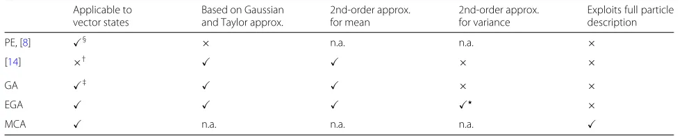
Additionally, the GA scheme is extended to a full second-order Taylor approximation. This method is henceforth called extended Gaussian approximation (EGA) and is intended to provide approximations that are more accurate than those obtained using GA. An overview of all discussed methods is given in Table1.
In the presented simulations, it is shown that the method proposed in this work outperforms all three methods considered for comparison, i.e., PE [8], GA (gen-eralized from [14]), and EGA, the last of which exploits full second-order approximations. Moreover, it is shown that the proposed method achieves higher localization accuracy within the same computing time.
1.3 Organization
This work is structured as follows. Section 2 intro-duces the concept of using MPF for tracking wireless agents. Section 3.1 presents the GA likelihood approx-imation technique. Sections 3.1.3 and 3.1.4 extend this scheme to present the EGA method. In Section 4, the proposed method is derived and presented. In Section5, the simulation setup and the performance met-ric are discussed. In Section 6, numerical results are presented, and all four considered methods are eval-uated and compared. Finally, conclusions are drawn in Section7.
2 Problem introduction and system model
This paper considers scenarios in which many wireless agents are localized using pairwise measurements, such as distance and/or bearing measurements. By the nature of the abovementioned scenarios (cf. Section1), a prede-fined and known number of agents are employed which are localized offline, after all agents’ readings have been extracted in a fusion center. Consequently, no uncertainty regarding the number of agents is considered. More-over, access to beacons is assumed to be available but limited, i.e., insufficient for agents to be accurately local-ized solely by utilizing beacon-to-agent measurements. For this reason, measurements between mobile agents (AAMs) become increasingly relevant.
Because distance and bearing measurements as well as realistic agent motions are nonlinear, PF approaches are considered in this work. Subsequently, the important properties of such approaches are briefly summarized.
In [27], the convergence of Monte Carlo approximation in terms of the mean square error was shown to be of O(L−1), where L is the number of particles. Moreover, it has been shown that the error is (in theory) indepen-dent of the state dimensionality. In practice, however, the dimensionality plays a significant role in determining the performance of PF techniques [3, 28]. For example, [3] reported an exponential relationship between the number
Table 1Features of the considered likelihood approximation schemes
Applicable to
§Uses point estimates only
†Equations are given only for scalar states ‡Generalization of [14] to vector states
of particles and the state dimensions (“curse of dimen-sionality”). Due to the high state-space dimensionality, classical PF approaches demand unreasonable resources for tracking many agents. Consequently, the concept of multiple particle filtering, in which one filter is used for each agent to be tracked, is considered instead.
A brief summary of the concepts relevant to particle filter (PF) and multiple particle filter (MPF) is presented below.
2.1 Particle filtering
In an agent tracking scenario, the objective is to sequen-tially estimate the agents’ states, which are assumed to be Markovian and discrete in time. Correspondingly, the following state-space model for agentiis considered:
xi,k+1= ˜f(xi,k,vk), yi,k = ˜h crete timekandyi,k ∈ Rnyrepresents the corresponding
measurements of this agent, each of which, by the nature of AAMs, also depends on the state vector of the other agent involved in that measurement,xj,k(henceforth, the notation j will be used to denote an agent other than i). Moreover, vk and ηk denote the process noise and measurement noise, respectively. The generally nonlin-ear functionsf˜(·)andh˜(·)denote the state evolution and measurement models, respectively, with noise included.
Equivalently, (1) can be written as
xi,k ∼p(xi,k|xi,k−1), (2a) yi,k ∼p(yi,k|xi,kxj,k). (2b)
In the context of sequential Bayesian filtering in general and the tracking of wireless agents in particular, the objec-tive is to recursively estimate the posterior distribution
p(xi,k|yi,1:k)=
For general nonlinear state-space models, these integrals cannot be computed analytically.
In sequential importance resampling (particle filter-ing), the posterior distribution p(xi,k|yi,1:k) is therefore approximated using L weighted particles, denoted by
denotes a particle index. The weights are defined as
w()i,k ∝ p A PD is used because in most cases, directly sampling fromp(xi,0:k|yi,1:k)is impossible because it would require solving complex and high-dimensional integrals for which no general analytical solution is known [28].
If the PD is chosen to be factorized such that [29]
π(x0:k|y1:k)=π(xk|x0:k−1,y1:k)π(x0:k−1|y1:k−1)
then the following recursive expression for the weights can be obtained [28]:
w()i,k ∝w()i,k−1
pyi,kx()i,kpx()i,kx()i,k−1 πx()i,kx()i,0:k−1,yi,1:k
. (7)
The performance of a PF scheme depends on the choice of the PDπ(·)and, as discussed in Section2, on the num-ber of particlesL. Regarding the former, it is known that an incremental variance-optimal PD is given by
π(xi,k|xi,0:k−1,yi,1:k)=p(xi,k|xi,k−1,yi,1:k);
however, in most cases, this PD is not available for sam-pling [30]. This is because, in the general case, such sampling would require solving an integral without an analytical solution. Consequently, in many cases, the PD is chosen to be
π(xi,k|xi,0:k−1,yi,1:k)=p(xi,k|xi,k−1), (8)
which further simplifies the PF (cf. (7)).
2.2 Multiple particle filtering
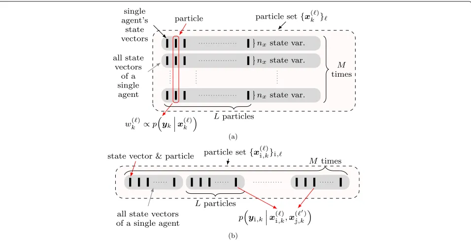
Fig. 1Illustrations ofaclassical andbMPF particle representations, wherenxdenotes the dimension of the state vectors
By contrast, in MPF, a separate PF is employed for every agent, resulting in the particle representation illustrated in Fig.1b. The benefits are a reduced state dimensionality on a per-PF basis and the resulting improved conver-gence properties. However, the separation of the PFs in MPF causes the likelihood, which is required to com-pute the weight update, for example (cf. (7)), to depend on two particles representing two parallel, decoupled PFs (i.e., the likelihood is nonseparable). In fact, in the con-text of distance- and/or bearing-based tracking in our scenario, the likelihood is nonseparable for the following two reasons: first, the necessity of considering agent-to-agent measurements, and second, the fact that both types of measurements inherently depend on the states of both agents conducting the measurements and their corresponding filters.
In terms of likelihoods, the use of MPF in the context of distance- and/or bearing-based tracking is associated with the following problem: In MPF, onlyp(yi,k|xi,k,xj,k) is readily available, wherexi,k andxj,k are described by particles of different PFs. However, for the weight update in each PF (cf. (7) and line5in Algorithm 1), the full like-lihood p(yi,k|xi,k) is required. Therefore, special proce-dures are required to approximate the required likelihood. The proposal of new procedures for this task is the main topic of this work.
To this end, the following sections discuss three differ-ent techniques for approximatingp(yi,k|xi,k)for each PF based on the particle information from all parallel PFs {p(yi,k|xi,k,xj,k)}i.
3 Gaussian likelihood approximation via Taylor
approximation
The general idea presented in [14] is to approximate the sought likelihoodp(yi,k|xi,k) by a Gaussian distribution, leaving only the meanE[yi,k|xi,k] and varianceV[yi,k|xi,k] to be computed. In this case,xj,k is treated as a random variable, and its moments are deduced from the particles. The scalar measurements are subsequently assumed to result fromh˜(·):
yi,k= ˜h(xi,k,xj,k,ηk), (9)
via Taylor expansion of the measurement function around the mean of xj,k. In [14], corresponding equations for scalar statesxi,k andxj,kare given under the assumption
Algorithm 1:Outline of multiple particle filtering
1 Sample priorp(xi,0)for all agents;
2 foreachk=1,. . .,Kdo // Loop over all time
steps
3 foreachi=1,. . .,Mdo // Loop over all
agents
4 Time update using PD, cf. (8);
5 Weight update, cf. (7), for which an approximation top(yi,k|xi,k)is required;
6 Resampling;
of additive measurement noise and for first-order approx-imations of the variance only. In the remaining part of this section, this approach will be extended to cover the gen-eral case of vector states that is required for the described application case. With this approximation of the bootstrap filter, the weights are updated (cf. (7)) using:
pyi,k|x()i,k
Subsequently, the derivations for additive white Gaus-sian noise (AWGN)- and multiplicative GausGaus-sian noise-corrupted measurement are given in Sections 3.1.3and 3.1.4, respectively. Note that both approximations are needed due to the assumption of multiplicative Gaus-sian noise- and AWGN-corrupted distance and bearing measurements, respectively.
3.1 Taylor approximation
First, consider the following noise-free measurements:
yi,k =h(xi,k,xj,k). (11)
Subsequently, a second-order Taylor approximation around the mean ofxj,kis derived forh(xi,k,xj,k). uated atx¯j,k, which are henceforth denoted simply byg andH, respectively.
3.1.1 First moment of Taylor approximation
Lemma 1(Expectation value of a quadratic form [31]) Letμ=E[x]and=Cov[x]; then,
E[xAx]=tr[A]+μAμ, (13)
whereAis a real square matrix.
The conditional expectation value of the Taylor approx-imanthˆ(·)(cf. (12)) can be derived by using Lemma1in
Lemma 2 (Covariance of a quadratic form [32])Letx be multivariate Gaussian with mean μ and covariance matrix; then,
CovxAx=2tr(A)2+4μAμ, (15) where(A)2=AAandAis a real square matrix.
3.1.2 Second moment of Taylor approximation
Based on Eq.13, the second noncentral moment can be calculated as follows:
where the last summand in (16) can be simplified using
E x˜ assumption of Gaussian states xj,k is made. Moreover, under the same assumptions, AppendixAshows that the third-order moment in Eq.16vanishes; that is:
Egx˜j,kx˜j,kHx˜j,kxi,k
=0.
Consequently, the second noncentral moment is described by
3.1.3 Synthesis: Additive white Gaussian noise measurements
For AWGN-corrupted measurements of the form:
yi,k =h
the desired moments can be found as follows:
Vyi,kxi,k
3.1.4 Synthesis: Multiplicative Gaussian noise measurements
Similarly, in the case of multiplicative noise in the form
yi,k=h
The variance can again be obtained via (22).
4 Monte Carlo-based likelihood approximation
In the following, a Monte Carlo (MC)-based approxima-tion of the sought likelihood is derived. This approxi-mation is believed to be more accurate than the pre-sented GA-based methods because it does not rely on the assumption that the corresponding likelihood can be modeled by a Gaussian distribution. Moreover, our MCA method does not exploit only the first- and second-order statistics of the particles; instead, it uses the complete information carried by the particles.
The derivation is based on the following approximation of the sought likelihood:
where()is given by the Chapman-Kolmogorov equation and consequently can be computed as follows:
pxj,kyj,1:k−1 surements of agentiand the collection of past measure-ments of agent j are approximately conditionally inde-pendent given the current state of agent i. Using the
importance sampling description of the previous poste-rior,pxj,kyj,1:k−1
where the particle-based posterior description was used in step(§). Thus, the sought likelihood can be written as follows (cf. (26)):
Because the integral cannot be analytically computed in general, MC integration techniques are adopted, i.e., the integral is approximated as follows:
pyi,kx()i,k,xj,k dency on the particle . Finally, the likelihood that is sought is obtained as follows:
p
Because additional sampling and corresponding evalua-tions of the probability density function given in (32) is computationally demanding, a simplification is proposed: Instead of sampling new particlesx(j,nk|) as per (31), the time update samples (34), which are sampled from the same probability density function, are reused. With this procedure, approximation (35) is obtained which can be interpreted as a particular instance of (32) for n = 1. Therefore, an easily implementable approximation of the sought likelihood is obtained that avoids the computation of gradients and Hessians, which are needed in GA-based methods. The full bootstrap-like algorithm employing the proposed approximation is described in Algorithm 2, whereAyi,idenotes the set of agents from which
Algorithm 2: Particle Filter with proposed Likelihood Approximation for Multiple Particle Filter
input : Prior, evolution and measurement densitiesp(xi,0), p(xi,k|xi,k−1), andp(yi,k|xi,kxj,k)
4 Draw samplesx()i,kfrom the importance distribution
x()i,k∼pxi,kx()i,k−1
8 Calculate new weights according to
γ
10 Obtain unnormalized weights as
w()i,k←w()i,k−1 j∈Ayi,i
γ
j (36)
and normalize them to sum to unity via
w()i,k←w
5 Simulation setup and method
This section introduces the chosen simulation setups, including the environment, as well as the state evolution and measurement models.
5.1 System model
Although the proposed procedure is also applicable to other models, the following Gaussian constant-velocity, constant-turn model is considered here for each agent, with xi,k+1 = f(xi,k) + νk = tions, respectively;vi,k =
˙
x2i,k+ ˙y2i,kis the agent’s speed; andφi,k = atan(y˙i,k/x˙i,k)andωi,k = ˙φi,k are the agent’s heading angle and turning rate, respectively.
The process noiseνk ∼ N(0,)is Gaussian, with the standard deviations of the noise processes that corre-spond to the linear acceleration and angular acceleration, respectively.
Consequently, it is assumed that p(xi,k|xi,k−1) =
N(f(xi,k−1),), wheref(·) is the noise-free state evolu-tion model given in Eq.38.
In the following, bearing and distance measurements between agents or beaconsiandjof the form
yi,j,k= (xi,k−xj,k)2+(yi,k−yj,k)2·(1+ηd,k) atan2(yi,k−yj,k, xi,k−xj,k)+ηb,k
(40)
are considered, whereηk =[ηd,k,ηb,k]∼ N(0,), with
= diag(σd2,σb2), where σd and σb are the standard deviations of the noise in the distance and the bearing measurements, respectively. The multiplicative model for the distance measurements accommodates the observa-tion that distance measurements made with respect to farther agents are less accurate.
The full measurement vector for agentiis then obtained as follows:
yi,k=. . . yi,j,k . . .. (41) To obtain the results presented in the following section, the sampling period was set toT = 1 s, and the process noise parameters were set toσ˙v=3.16×10⁻³m/s2,σω˙ = 3.16×10⁻³rad/s2, andσx=σy=0.30 m.
5.2 Simulation setup I
The first simulation setup is visualized in Fig. 2. It con-sists of four mobile agents and four beacons, each with a sensing radius of 4 m. In this setup, multiple different maneuvers, consisting of turns and velocity changes, need to be captured. A variety of trajectories are used to test the algorithms’ performance on these two main types of maneuvers. The agents follow the model given in (38), but the turn rate and speed are abruptly changed.
Fig. 2Simulation setup with four agents and four beacons. The agents’ true trajectories are shown
Here, 0n and 1n denote a sequence of n zeros and a sequence ofn ones, respectively. Moreover,b
a denotes the sequence that yields aa·πturn inbsteps.
Due to the limited sensing range, this setup is rele-vant to the considered scenario of limited beacon access. All figures show results averaged over 100 simulations. All algorithms listed in Table2are evaluated. This table also summarizes the key features and properties of the algorithms.
The setup is chosen for the following reasons: First, the agents follow predefined trajectories that, apart from the introduced abrupt changes with respect to velocity and turn rate, are fully consistent with the chosen motion model (38). Consequently, any tracking inaccuracy result-ing from model mismatch, which will inherently arise in any real-world scenario, is strongly limited. This, in turn, facilitates a more in-depth analysis and fairer comparison of the different likelihood approximation methods, which target only the measurement function (cf. (2a)). Second, despite the use of predefined trajectories, the maneuvers are complex and challenging due to the variation in their motion profiles, which include a broad set of different turns and acceleration phases. Thus, adequate likelihood approximation schemes are required to enable accurate localization.
The reported results below are related to the following two measurement noise scenarios (MNSs):MNS 1: Multi-plicative measurement noise with a standard deviation of σd=0.04 and bearing measurement noise with a standard deviation ofσb=5◦andMNS 2:σd=0.06,σb=10◦.
5.3 Simulation setup II
Additional simulation results, in which the agents’ motion is obtained via computational fluid dynamics (CFD) simu-lations, are presented. In contrast to the results presented in the context of the first simulation setup, the resulting agent motion cannot, to a significant extent, be properly modeled by (38) (cf. Section5). For this reason, the results presented and discussed for this setup exhibit more vari-ation. The CFD results were obtained by simulating the pipe model shown in Fig.3using a D2Q9 lattice Boltz-mann model (LBM). The pipe is filled with water at 25 °C. The LBM parameters used for the CFD simulation are listed in Table 3. Details such as the boundary method implemented for the D2Q9 LBM are given in [34], where
Table 2Overview of the evaluated algorithms
Abbr. Proposed in
Discussed in
Comment
PE [8] — Eliminates the dependency of
the likelihood on the other agent’s state by means of the point estimate xjˆ,k = a Gaussian density using first-and second-order terms for the variance and mean,
respectively. Treatsxj,kas a
ran-dom variable in the
Extension of GA to a complete second-order approx. for both additive and multiplicative noise.
MCA This
work
Fig. 3Four agents (turquoise) in a pipeline. This setup was used for CFD simulations with dimensions of 11.2 m×6.48 m and four beacons (red diamonds). The different colors (blue to yellow) indicate different speeds, and the arrows indicate the direction of the flow. The figure shows the velocity normalized to the max. occurring velocity
this method is reported to be accurate to approximately second order.
These simulation results are thus consistent with the application scenarios discussed in Section 1, in which miniature agents may be employed to survey underground structures or pipeline systems, such as those that exist in chemical plants. The chosen setup, however, is designed to challenge the algorithms (cf. Table2), which is achieved through a combination of fast agent motion and limited beacon coverage.
5.4 Evaluation metric
The following time- and agent-averaged localization error metric is used to evaluate the algorithms’ performance: MAE = M1·K Mi=1Kk=1pi,k− ˆpi,k2, wherepi,k is the true position of agentiat time stepkandpˆi,k is the cor-responding estimate, which refers to the first two states of the corresponding state vector.
6 Numerical results and discussion
The discussion of the simulation results is split into three main parts, with each focusing on different behavior and properties of the methods. This discussion is presented in the following subsections.
Table 3D2Q9 LBM simulation parameters
Parameter Value
LBM relaxation time 0.515
LBM speed 0.05
Max. LBM iterations 1×10⁴
LBM convergence threshold 1×10⁻⁷
Viscosity [m2/s] 0.89×10⁻⁶
Density [kg/m3] 997.05
For all results evaluating a performance as a function of particles per agent (PPA), the 99% confidence inter-vals (CIs) are shown as well. These results are visualized as a transparent hose around the average performance with the same line style and visualize the variation in the individual simulations.
6.1 Setup I: Localization error vs. number of particles and run time
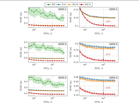
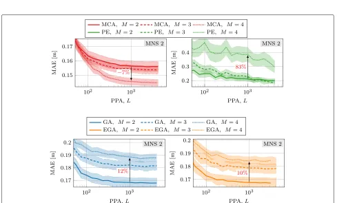
The first set of results is presented in Fig.4, which shows the localization performance as a function of the number of PPA,L. MNS 1 and MNS 2 are represented in the top and middle panels, respectively. Moreover, in Figs.4and5, a third MNS is presented in which multiplicative distance measurement noise is increased toσd= 0.1 compared to MNS 2.
The left panels of Fig.4 clearly show that PE exhibits significantly reduced performance compared to that of the other three methods. The right row of Fig.4focuses on the differences between the GA-based algorithms (GA and EGA) and the proposed MCA method. In these pan-els, the differences between the former two are generally small. However, the performance of MCA is significantly improved compared to that of the other methods. For example, forL = 1000, an error reduction of 16% com-pared to EGA is achieved. The middle panels show that in MNS 2, EGA is slightly superior to GA. Most notably, the localization error reduction of 21% is achieved by MCA over EGA. Similarly, for MNS 3, MCA achieves error reductions of 24%.
Interestingly, the mean absolute error (MAE) of the PE method decreases from 0.46 (MNS 1) to 0.39 (MNS 2) to 0.35 (MNS 3) with increased measurement noise. In contrast, the MAE of the other methods increases at the same time. For example, for MCA, the MAE increases from 0.10 to 0.15 to 0.18 at these measurement noise con-figurations. Despite this increase in absolute terms, the relativeimprovement of MCA over EGA increases from 16% (MNS 1) to 22% (MNS 2) to 24% (MNS 3), as men-tioned above. Importantly, despite the improvement in PE with increasing noise intensity, the absolute performance gains through MCA remain significant. Additionally, CIs show that the performance of PE is the least consistent.
Fig. 4Localization error as a function of PPA. The plots for MNS 1, MNS 2, and MNS2 3 are at the top, middle, and bottom, respectively. In all panels, M=4 agents are considered. The right panels show magnified views of the results presented in the upper panels but without the PE results for improved readability
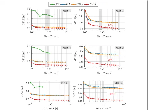
or computing time. Similar to the previous results, the left panels of Fig. 5 show a comparison among all four algorithms, whereas the right panels of Fig. 5 focus on the GA-based methods and MCA. Because the results in Fig.5 are deduced from the data depicted in Fig.4, the supports for the curves are different. As such, the left pan-els of Fig.5show low run times for PE because no data are available for run times longer than 10 s. However, these low run times are not accompanied by performance values better than a localization error of 0.34 m.
The right panels of Fig.5(together with the right panels of Fig.4) show that MCA not only yields improved local-ization performance, with a lower locallocal-ization error than those of all other methods, but also achieves improved performance within the same computing time. For exam-ple, in MNS 1, a reduction in the error metric of 14% is achieved for a run time of 14 s. Similarly, for MNS 2 and MNS 3, reductions in 20% and 23% are obtained, respectively.
6.2 Setup I: Performance over time
The second set of results, illustrating the performance of the algorithms over the different time steps, is visualized in Figs.6, and7.
Figure 6 visualizes the performance for MNS 2 with 422 PPA, which has been chosen as a compromise between a low PPA (where MCA performs similarly to EGA) and a high PPA (where MCA is able to signifi-cantly improve compared to EGA and the other meth-ods). The estimated positions are overlaid on the agents’ actual trajectories, which are shown in red, and are plotted as markers only in the same colors as those used in Fig.2.
Fig. 5Localization error as a function of run time. The plots for MNS 1 and MNS 2 are at the top and bottom, respectively. In both MNSs,M=4 agents are considered. The right panels show magnified views of the results presented in the upper panels but without the PE results for improved readability
reduction of almost 50% in the localization error. How-ever, both of these algorithms also show reduced tracking accuracy during maneuvers (cf. in particular the estimates represented by red markers in the top loop and by green and orange markers at the saddle points of the maneu-vers). Figure6a shows the performance of MCA, which encounters only minor issues with tracking (cf. the esti-mates represented by red markers in the top loop). This superior performance is also evident from the reduction of−22% in the localization error compared with that of GA.
Figure7b clearly shows a decreasing tracking accuracy, with the peak being in the transition zone between the coverage areas of the left and right beacons. Figure 7c and d, for GA and EGA, respectively, show significantly improved performance compared with that of PE, with some strong fluctuations (note the differences in scal-ing for reasons of readability). Figure 7a shows the per-formance of MCA. At the beginning of tracking, MCA
exhibits a significant reduction in error from the initial value. Compared to all other methods, not only reduced error but also lower fluctuations in the performance over time are apparent.
6.3 Setup I: Localization error vs. number of agents
The third and last set of results for the first setup is presented in Figs.8and9, which analyze the tracking per-formance for varying numbers of agents for MNS 1 and MNS 2, respectively. The results were obtained with the same setup depicted in Fig. 2, with only the first i = 1,. . .,Magents being simulated in cases with fewer than four agents.
Fig. 6Estimated averaged trajectories (markers only) for all methods, with the actual trajectories underlaid in black (cf. Fig.2). These results were obtained for MNS 2 and 422 PPA
Fig. 8Localization error as a function of the number of PPA for different numbers of agents to be tracked for MNS 1
Fig. 10Localization performance as a function of PPA for different numbers of agents:afour agents,bsix agents,ceight agents, anddten agents
error metric decreasing by approximately 2% in the same case.
Similar trends can be observed in Fig. 9 for increas-ing measurement noise. Here, the error metric of MCA is reduced by 6.88% when four agents are tracked instead of two.
In both MNSs, this behavior can be explained by the additional agent-to-agent measurements that are pro-vided by the additional agents. In the cases of GA and EGA, for example, these additional measurements result in significant error accumulation because the likelihoods are approximated as Gaussian distributions and, in the weight update (cf. (7)), the product of these likelihoods is taken3. For MCA, however, the approximation error is lower, allowing the additional measurements provided by the extra agents to be successfully exploited.
6.4 Setup II: Localization error vs. number of particles and run time
For brevity, the second setup is evaluated only for the fol-lowing simulation configuration. The MNS was scenario 2, and the agent and beacon coverage ranges were both Rs=10 m.
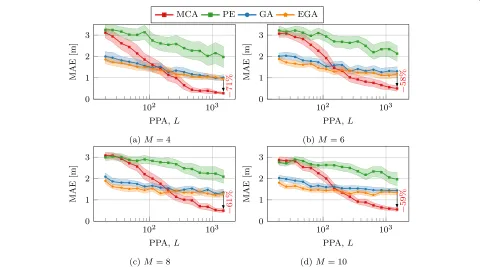
The first set of results is presented in Fig. 10, which compares the performance of the different algorithms as a function of the number of PPA. The different panels of
3Recall that the measurement noise is assumed to be independent and
identically distributed in nature.
Fig.10present the results forM= 4, 6, 8, and 10 agents. For low PPA values, GA and EGA outperform MCA. However, GA and EGA do not achieve a MAE lower than 1 m, which can be considered critical depending on the precise application requirements. For more than approx. 200 PPA, MCA achieves the best performance, resulting in MAE reductions of between 71% (forM=4) and 59% (forM=10) compared to EGA. Interestingly, not only the average MAE performance of MCA improves for increas-ing PPA: For example, for four agents, the size of the CI for MCA decreases from 0.55 m (200 PPA) to 0.08 m (1500 PPA). Similarly, for ten agents, the CI size decreases from 0.32 m to 0.17 m at the same time.
Similar to the results discussed in Section6, EGA out-performs GA, although marginally, throughout the simu-lations.
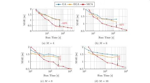
The second set of results is given in Fig.11, which com-pares the run times of the algorithms with their achieved MAE values. With the same run-time budget, the follow-ing reductions in MAE are achieved: forM=4 agents and 62 s, 63%; forM = 6 agents and 145 s, 32%; forM = 8 agents and 254 s, 45%; and forM=10 agents and 389 s, a reduction of 45%.
6.5 Setup II: Localization error vs. number of agents
Fig. 11Localization performance as a function of run time for 1500 PPA and for different numbers of agents:afour agents,bsix agents,ceight agents, anddten agents
variations in the number of agents and the PPA value for MCA are very low in the absolute sense. In fact, the per-formance degradation associated with the requirement to track 10 instead of 4 agents corresponds to an increase of only approximately 0.27 m relative to the initial value of 0.275 m (M=4). In contrast, not only the fluctuations but also the absolute MAE values for GA and EGA are much higher. For example, for 1500 PPA, the MAE increases by 0.43 m from an initial value of 1 m (GA) and by 0.4 m from an initial value of 0.95 m (EGA).
The fourth and final set of results is presented in Figs.13 and14, which show the actual agents’ trajectories as solid lines and the average estimated positions as markers only forM=4 and 8 agents, respectively. ForM=4 agents (cf. Fig.13), MCA can accurately track the agents’ fast motion and achieves an average MAE of 0.28 m. In contrast, the other methods quickly lose track of the agents’ motion and cannot achieve an MAE better than 0.95 m.
In the case that 8 agents are to be tracked (cf. Fig.14), MCA tends to overestimate the turn rates of the agents, resulting in an average MAE of 0.5 m. In contrast, all other methods are, on average, unable to track the agents’ motion at all, resulting in a poor accuracy of 1.28 m at best.
6.6 Setup II: Summary of results
In the second simulation setup, a close-to-reality sce-nario is considered in which up to 10 agents are car-ried by fluid dynamics alone through a pipe branch.
Because the agents’ motion is difficult to describe with a single motion model, the results, as expected, show more fluctuations and are more dependent on the accu-racy of the motion model compared to results of the first simulation setup. Nevertheless, even in this sce-nario, the proposed MCA method outperforms the PE, GA, and EGA methods, achieving MAE reductions of up to 63% when the computational costs for all methods are fixed.
7 Conclusion and future work
Fig. 12Localization performance as a function of the PPA value and as a function of the number of agents to be tracked.aMCA.bPE.cGA.dEGA
Fig. 13Average estimated positions (markers) and actual trajectories (solid lines) in the case ofM=4 agents and for 1500 PPA.aMCA, MAE 0.28 m.
Fig. 14Average estimated positions (markers) and actual trajectories (solid lines) in the case ofM=8 agents and for 1500 PPA.aMCA, MAE 0.50 m.
bPE, MAE 2.09 m.cGA, MAE 1.35 m.dEGA, MAE 1.28 m
additional measurements introduced with an increase in the number of agents to be tracked in the synthetic bench-mark (first setup). Similarly, for the second set of close-to-reality simulations (second setup), MCA was least affected by an increase in the number of agents. In numbers, MCA achieved MAE reductions between 58 and 71% compared to EGA.
In summary, the MCA scheme presented in this study offers significant improvements in localization accuracy and/or computing time. The scheme has shown poten-tial for many application cases in which a known number of cooperating agents are to be localized using distance and/or bearing measurements if access to beacons is lim-ited and/or AAMs are essential for accurate localization. Examples thereof are rescue robots employed for survey-ing collapsed buildsurvey-ings due to earthquakes and miniature agents used for pipeline inspection.
In future works, we will investigate the proposed scheme on a broader scale, including the effect of the MC parameter n on performance and run time. More-over, an in-depth theoretical analysis of the computational complexity of all discussed algorithms is of interest in this context.
Appendix A: Proof of the third-order moment of a Gaussian approximation component
As mentioned in Section3, the statex˜j,k is assumed to be Gaussian. For simplicity, the agent and time indices are
dropped in the following, such thatx˜j,k = ˜xandxi,k =x. Generally, thei-th element of a vectorxis denoted by [x]i, and the(i,j)-th element of a matrixXis denoted by [X]i,j. For simplicity, [x˜j,k]iis denoted byx˜i.
With this new notation,
Egx˜j,kx˜j,kHx˜j,kxi,k
=
i
j
l
gi[H]j,lE[x˜ix˜jx˜l|xi,k] ,
(42)
and the expected value that is sought reduces to the sum of the higher-order moments of a Gaussian random vector. Subsequently, the link between the higher-order moments and the multivariate Hermite polynomials is exploited in accordance with the following theorem.
Theorem 1 (Higher-order moments of multivariate Gaussian random variables [35])For a Gaussian random vectorx∼ N(μ,), withμ∈ Rnand ∈ Rn×n 0, it holds that
Exν1 1 · · ·xνnn
=Heν1,...,νn(−
−1μ,−), (43)
where theνiare nonnegative integers. The Hermite polyno-mials are defined as
Heν1,...,νn(z,A)=exp(Q/2)
n
i=1
!
−∂∂ zi
"νi
exp(−Q/2),
(44)
Noting thatx˜is zero-mean by definition, it holds that
The following three cases need to be addressed for (42), without loss of generality:i=j=l,i=j=l, andi=j= l. For all of them, the following derivative is important:
∂ Covariance matrix with respect to densityp;δ(x−x0): Dirac delta function centered atx0;Ep[·]: Expectation operator with respect to densityp;i,j,: Some agent indices;L: Number of particles;: Particle index; [X]i,j:(i,j)-th element of matrixX;η: Measurement noise vector;N(μ,): Normal distribution with meanμand covariance matrix;ν: Process noise vector; O(·): Computational complexity in terms of big O notation;p(·): Probability density function or probability mass function;b
a: Sequence that yields aa·π Cartesianycoordinate of agentiat time stepk
Abbreviations
AAM: Agent-to-agent measurement; AWGN: Additive white Gaussian noise; CFD: Computational fluid dynamics; CI: Confidence interval; EGA: Extended Gaussian approximation; GA: Gaussian approximation; LBM: Lattice Boltzmann model; MAE: Mean absolute error; MC: Monte Carlo; MCA: Monte Carlo approximation; MNS: Measurement noise scenario; MPF: Multiple particle filter;
PD: Proposal distribution; PE: Point-estimate approximation; PF: Particle filter; PPA: Particles per agent; RFS: Random finite set
Acknowledgments
We gratefully acknowledge the computational resources provided by the RWTH Compute Cluster from RWTH Aachen University under project RWTH0118.
Authors’ contributions
SS performed the simulations and wrote the majority of the manuscript. GA initiated the research and also commented on and approved the manuscript. Both authors read and approved the final manuscript.
Authors’ information
All authors are with the Chair for Integrated Signal Processing Systems, RWTH Aachen University, Germany. Email addresses:
[email protected], [email protected]
Funding
This project has received funding from the European Union’s Horizon 2020 research and innovation program under grant agreement No. 665347.
Availability of data and materials
Not applicable.
Competing interests
The authors declare that they have no competing interests.
Received: 29 April 2019 Accepted: 2 September 2019
References
1. S. Schlupkothen, G. Dartmann, G. Ascheid, A novel low-complexity numerical localization method for dynamic wireless sensor networks. IEEE Trans. Signal Process.63(15), 4102–4114 (2015).https://doi.org/10.1109/ TSP.2015.2422685
2. S. Schlupkothen, A. Hallawa, G. Ascheid, in2018 International Conference on Computing, Networking and Communications (ICNC): Wireless Ad Hoc and Sensor Networks (ICNC’18 WAHS). Evolutionary algorithm optimized centralized offline localization and mapping (IEEE, Maui, 2018) 3. F. Daum, J. Huang, in2003 IEEE Aerospace Conference Proceedings (Cat.
No.03TH8652). Curse of dimensionality and particle filters, vol. 4, (2003), pp. 1979–1993.https://doi.org/10.1109/AERO.2003.1235126 4. F. Gustafsson, F. Gunnarsson, N. Bergman, U. Forssell, J. Jansson, R.
Karlsson, P. J. Nordlund, Particle filters for positioning, navigation, and tracking. IEEE Trans. Signal Process.50(2), 425–437 (2002).https://doi.org/ 10.1109/78.978396
5. D. Chang, M. Fang, Bearing-only maneuvering mobile tracking with nonlinear filtering algorithms in wireless sensor networks. IEEE Syst. J.8(1), 160–170 (2014).https://doi.org/10.1109/JSYST.2013.2260641
6. P. Yang, Efficient particle filter algorithm for ultrasonic sensor-based 2D range-only simultaneous localisation and mapping application. IET Wirel. Sensor Syst.2(4), 394–401 (2012).https://doi.org/10.1049/iet-wss.2011. 0129
7. B. F. Wu, C. L. Jen, Particle-filter-based radio localization for mobile robots in the environments with low-density WLAN APs. IEEE Trans. Ind. Electron.
61(12), 6860–6870 (2014).https://doi.org/10.1109/TIE.2014.2327553 8. P. M. Djuric, T. Lu, M. F. Bugallo, in2007 IEEE International Conference on
Acoustics, Speech and Signal Processing - ICASSP ’07. Multiple particle filtering, vol. 3, (2007), pp. 1181–1184.https://doi.org/10.1109/ICASSP. 2007.367053
9. M. F. Bugallo, T. Lu, P. M. Djuric, in2007 IEEE Aerospace Conference. Target tracking by multiple particle filtering, (2007), pp. 1–7.https://doi.org/10. 1109/AERO.2007.353042
10. M. F. Bugallo, P. M. Djuri´c, in2010 IEEE Aerospace Conference. Target tracking by symbiotic particle filtering, (2010), pp. 1–7.https://doi.org/10. 1109/AERO.2010.5446681
12. M. F. Bugallo, P. M. Djuri´c, in2014 IEEE Workshop on Statistical Signal Processing (SSP). Gaussian particle filtering in high-dimensional systems, (2014), pp. 129–132.https://doi.org/10.1109/SSP.2014.6884592 13. M. F. Bugallo, P. M. Djuri´c, in2014 IEEE International Conference on
Acoustics, Speech and Signal Processing (ICASSP). Particle filtering in high-dimensional systems with gaussian approximations, (2014), pp. 8013–8017.https://doi.org/10.1109/ICASSP.2014.6855161 14. P. M. Djuri´c, M. F. Bugallo, in2015 IEEE International Conference on
Acoustics, Speech and Signal Processing (ICASSP). Multiple particle filtering with improved efficiency and performance, (2015), pp. 4110–4114. https://doi.org/10.1109/ICASSP.2015.7178744
15. L. Martino, J. Read, V. Elvira, F. Louzada, Cooperative parallel particle filters for online model selection and applications to urban mobility. Digit. Signal Process.60, 172–185 (2017).https://doi.org/10.1016/j.dsp.2016.09.011 16. I. Urteaga, M. F. Bugallo, P. M. Djuri´c, in2016 IEEE Statistical Signal
Processing Workshop (SSP). Sequential Monte Carlo methods under model uncertainty, (2016), pp. 1–5.https://doi.org/10.1109/SSP.2016.7551747 17. J. A. Hoeting, D. Madigan, A. E. Raftery, C. T. Volinsky, Bayesian model
averaging: a tutorial. Stat. Sci.14(4), 382–401 (1999)
18. B.-N. Vo, S. Singh, A. Doucet, Sequential Monte Carlo methods for multitarget filtering with random finite sets. IEEE Trans. Aerosp. Electron. Syst.41(4), 1224–1245 (2005).https://doi.org/10.1109/TAES.2005.1561884 19. M. B. Guldogan, Consensus bernoulli filter for distributed detection and
tracking using multi-static doppler shifts. IEEE Signal Process. Lett.21(6), 672–676 (2014).https://doi.org/10.1109/LSP.2014.2313177
20. S. Reuter, K. Dietmayer, in14th International Conference on Information Fusion. Pedestrian tracking using random finite sets, (2011), pp. 1–8 21. W.-K. Ma, B.-N. Vo, S. S. Singh, A. Baddeley, Tracking an unknown
time-varying number of speakers using TDOA measurements: a random finite set approach. IEEE Trans. Signal Process.54(9), 3291–3304 (2006). https://doi.org/10.1109/TSP.2006.877658
22. A. Eryildirim, M. B. Guldogan, A Bernoulli filter for extended target tracking using random matrices in a UWB sensor network. IEEE Sensors J.16(11), 4362–4373 (2016).https://doi.org/10.1109/JSEN.2016.2544807 23. P. Biswas, Y. Ye, inInformation Processing in Sensor Networks, 2004. IPSN
2004. Third International Symposium On. Semidefinite programming for ad hoc wireless sensor network localization, (2004), pp. 46–54.https://doi. org/10.1109/IPSN.2004.1307322
24. P. Biswas, T.-C. Liang, K.-C. Toh, Y. Ye, T.-C. Wang, Semidefinite programming approaches for sensor network localization with noisy distance measurements.3(4), 360–371 (2006).https://doi.org/10.1109/ TASE.2006.877401
25. P. Biswas, T.-C. Lian, T.-C. Wang, Y. Ye, Semidefinite programming based algorithms for sensor network localization. ACM Trans. Sen. Netw.2(2), 188–220 (2006).https://doi.org/10.1145/1149283.1149286
26. S. Schlupkothen, G. Ascheid, in2016 IEEE International Conference on Wireless for Space and Extreme Environments (WiSEE) (WiSEE’16). Joint localization and transmit-ambiguity resolution for ultra-low energy wireless sensors, (2016).https://doi.org/10.1109/wisee.2016.7877302 27. D. Crisan, A. Doucet, A survey of convergence results on particle filtering
methods for practitioners. IEEE Trans. Signal Process.50(3), 736–746 (2002).https://doi.org/10.1109/78.984773
28. S. Särkkä,Bayesian Filtering and Smoothing. (Cambridge University Press, New York, 2013)
29. A. Doucet, A. Smith, N. de Freitas, N. Gordon,Sequential Monte Carlo Methods in Practice, ser. Information Science and Statistics. (Springer, 2001). https://doi.org/10.1007/978-1-4757-3437-9
30. A. Doucet, S. Godsill, C. Andrieu, On sequential Monte Carlo sampling methods for Bayesian filtering. Stat. Comput.10(3), 197–208 (2000). https://doi.org/10.1023/A:1008935410038
31. A. M. Mathai, S. B. Provost,Quadratic Forms in Random Variables, ser. Statistics: A Series of Textbooks and Monographs. (Taylor & Francis, 1992) 32. A. C. Rencher, G. B. Schaalje,Linear Models in Statistics. (Wiley, 2008) 33. X. R. Li, V. P. Jilkov, Survey of maneuvering target tracking. Part I. Dynamic
models. IEEE Trans. Aerosp. Electron. Syst.39(4), 1333–1364 (2003). https://doi.org/10.1109/TAES.2003.1261132
34. Q. Zou, X. He, On pressure and velocity boundary conditions for the lattice Boltzmann BGK model. Phys. Fluids.9(6), 1591–1598 (1997). https://doi.org/10.1063/1.869307
35. C. S. Withers, The moments of the multivariate normal. Bull. Aust. Math. Soc.32(1), 103–107 (1985).https://doi.org/10.1017/S000497270000976X
Publisher’s Note