R E S E A R C H
Open Access
On recovery of block-sparse signals via mixed
l
2
/
l
q
(
0
<
q
≤
1
)
norm minimization
Yao Wang
1, Jianjun Wang
2*and Zongben Xu
1Abstract
Compressed sensing (CS) states that a sparse signal can exactly be recovered from very few linear measurements. While in many applications, real-world signals also exhibit additional structures aside from standard sparsity. The typical example is the so-called block-sparse signals whose non-zero coefficients occur in a few blocks. In this article, we investigate the mixedl2/lq(0<q≤1)norm minimization method for the exact and robust recovery of such block-sparse signals. We mainly show that the non-convexl2/lq(0<q<1)minimization method has stronger sparsity promoting ability than the commonly usedl2/l1minimization method both practically and theoretically. In terms of a block variant of the restricted isometry property of measurement matrix, we present weaker sufficient conditions for exact and robust block-sparse signal recovery than those known forl2/l1minimization. We also propose an efficient Iteratively Reweighted Least-Squares (IRLS) algorithm for the induced non-convex optimization problem. The obtained weaker conditions and the proposed IRLS algorithm are tested and compared with the mixed l2/l1minimization method and the standardlqminimization method on a series of noiseless and noisy block-sparse signals. All the comparisons demonstrate the outperformance of the mixedl2/lq(0<q<1)method for block-sparse signal recovery applications, and meaningfulness in the development of new CS technology.
Keywords: Block-sparse recovery, Compressed sensing, Block-RIP,l2/lqminimization, IRLS
1 Introduction
According to the Shannon/Nyquist sampling theorem [1,2], if we would like to avoid lose of information when capturing a signal, we must sample the signal at the so-called Nyquist rate, which means twice the highest fre-quency of the signal. Since the theorem only exploits the bandlimitedness of a signal and most real-world signals are sparse or compressible, the process of massive data acquisition based on Shannon/Nyquist sampling theorem usually samples too many useless information and even-tually we have to compress to store or encode a very few essential information of the signal. Obviously, this process is extremely wasteful and therefore, a more effective sam-pling way to directly acquire the essential information of a signal has been expected.
Compressed sensing (CS) [3-5] was motivated by this purpose and it can completely acquire the essential
*Correspondence: [email protected]
2School of Mathematics and Statistics, Southwest University, Chongqing 400715, China
Full list of author information is available at the end of the article
information of a signal by exploiting its compressibil-ity. In a word, the main contribution of CS is that it presents a new efficient scheme to capture and recover the compressible or sparse signals at a reduced sampling rate far below the Nyquist rate. The basic principle of CS is that it first employs non-adaptive linear projec-tions to preserve the structure of the signal; then one can exactly recover these signals from a surprisingly small number of random linear measurements through a
non-linear optimization procedure (such asl1-minimization) if
the measurement matrix satisfies some suitable sufficient
conditions in terms ofrestricted isometry property (RIP,
[6]). Consequently, CS implies that it is indeed possible to acquire the data in already compressed form. Nowa-days, driven by a wide range of applications, CS and other related problems have attracted much interest in vari-ous communities, such as in signal processing, machine learning, and statistics.
Different from general sparse signals in conventional sense, some real-world signals may exhibit some addi-tional structures, i.e., the non-zero coefficients appear in
a few fixed blocks, we refer to these signals as block-sparse signals in this article. Such block-block-sparse signals arise in various application problems, say, DNA microar-rays [7,8], equalization of sparse communication channels [9], source localization [10], wideband spectrum sensing [11], and color imaging [12].
Using standard convex relaxation (l1-minimization) as
conventional CS framework for recovering the block-sparse signal does not exploit the fact that the non-zero elements of the signal appear in consecutive positions. Therefore, one natural idea is considering the
block version of l1-minimization, i.e., the mixed l2/l1
-minimization, to exploit the block-sparsity. Many
previ-ous works have shown that the mixedl2/l1-minimization
is superior to standardl1-minimization when dealing with
such block-sparse signals [13-15]. Huang and Zhang [13]
developed a theory for the mixed l2/l1-minimization by
using a concept called strong group sparsity and they
demonstrated that the mixed norm minimization is very efficient for recovering strongly group-sparse signals. Sto-jnic et al. [15] obtained an optimal number of Gaussian measurements for uniquely recovering a block-sparse
sig-nal through the mixedl2/l1norm minimization. By
gen-eralizing the conventional RIP notion to the block-sparse case, Eldar and Mishali [14] showed that if the
measure-ment matrixDhas the same restricted isometry constant
as that in the l1 case, then the mixed norm method is
guaranteed to exactly recover any block-sparse signals in the noiseless case. Furthermore, they also showed that the block-sparse signal recovery would be robust in the noisy case under the same recovery condition. Another common approach to deal with the block-sparsity prob-lem is by suitably extending the standard greedy meth-ods, such as orthogonal matching pursuit, iterative hard thresholding (IHT), and compressive sampling matching pursuit (CoSaMP), to the block-sparse case. In [16], the CoSaMP algorithm and the IHT algorithm were extended to the model-based setting, treating the block-sparsity as a special case. It was also shown that the new recovery algorithms demonstrate provable performance guarantees and robustness properties. Eldar et al. [17] generalized the notion of coherence to the block-sparse setting and proved that a block-version of the orthogonal matching pursuit (BOMP) algorithm can exactly recover any block-sparse signal if the block-coherence is sufficiently small.
In addition, the mixedl2/l1-minimization approach was
certified to guarantee successful recovery with the same condition on block-coherence. Ben-Haim and Eldar [18] examined the ability of greedy algorithms to estimate a block-sparse signal from noisy measurements. They derived some near-oracle results for the block-sparse ver-sion of greedy pursuit algorithms both in the adversar-ial noise and the Gaussian noise cases. Majumdar and Ward [19] used BOMP to deal with the block-sparse
representation-based classification problem. The validity and robustness of these new methods were theoretically proved.
In recent years, several studies [20-27] have showed that
the non-convexlq(0 < q < 1)minimization allows the
exact recovery of sparse signals from fewer linear
mea-surements than that by l1-minimization. Chartrand and
Staneva [21] provided a weaker condition to guarantee
perfect recovery for the non-convex lq (0 < q < 1)
minimization method using alqvariant of the RIP. They
obtained the number of random Gaussian measurements necessary for the successful recovery of sparse signals via
lq (0 < q < 1) minimization with high probability. Sun
[27] used the conventional RIP as in thel1case to prove
that wheneverqis chosen to be about 0.6796×(1−δ2k),
everyk-sparse signal can exactly be recovered vialq
min-imization, hereδ2kis the restricted isometry constant for
the measurement matrix. Xu et al. [24-26] considered a
specially important case (q = 1/2) of lq minimization.
They developed a thresholding representation theory for
l1/2minimization and conducted a phase diagram study
to demonstrate the merits ofl1/2minimization.
This article presents an ongoing effort to extend the
non-convex lq(0 < q < 1) minimization methodology
to the setting of block-sparsity. Specifically, we will study the performance of the block-sparse signal recovery via
the mixed l2/lq (0 < q < 1) norm minimization by
means of the block RIP (block-RIP). We first exhibit that
under similar RIP conditions with that in the standardlq
case, the mixed l2/lq recovery method can assuredly to
recover any block-sparse signal, irrespective to the loca-tions of non-zero blocks. In addition, the method is robust in the presence of noise. Our formulated recovery
con-ditions will show that the non-convexl2/lq(0 < q < 1)
minimization is superior to the convex l2/l1
minimiza-tion within block-RIP framework. Furthermore, we will compare the sparse signal recovery ability of the
non-convex l2/lq(0 < q < 1) method to the convex l2/l1
method and the standardlqmethod by conducting a series
of simulation studies. To the best of the authors’ knowl-edge, although Majumdar and Ward [12] first proposed
the non-convexl2/lq(0<q<1)method in CS literature
for color imaging and showed that thel2/l0.4minimization
has the best performance on some imaging experiments, their works were experimental in feature and lack of con-vincing theoretical assessment. As compared, our work not only highlights theoretical merits of the non-convex block optimization method, but also makes a more inten-sive study on the block-sparse signal recovery capabilities
for some different values ofqvia numerical experiments.
We begin with our study in Section 2,3 and 4 by pre-senting the problem setting. In Section 5, we establish
the sufficient conditions for the mixed l2/lq(0 < q <
recovery of block-sparse signals in terms of block-RIP. We also develop an efficient Iteratively Reweighted Least-Squares (IRLS) algorithm to recover block-sparse signals from given fewer measurements, which generalizes the
algorithm of [28] to the unconstrainedl2/lq(0 < q ≤ 1)
norm minimization case in Section 6. In Section 7, we
show that the non-convexl2/lq(0 < q < 1)method has
stronger block-sparsity promoting ability than the convex
l2/l1method and the standardlqmethod through a series
of simulations. Finally, we conclude the article in Section 8 with some useful remarks.
2 Block-sparsity
The conventional CS only consider the sparsity that the
signalxhas at mostknon-zero elements, and it does not
take into account any further structure. However, in many practical scenarios, the non-zero elements are aligned to blocks, meaning that they appear in regions. These signals are referred to the block-sparse signals. Mathematically
speaking, a block-sparse signalx ∈ RN over block index
setI= {d1,. . .,dm}can be modeled as follows:
x=[x 1· · ·xd1
x[1]
xd1+1· · ·xd1+d2
x[2]
· · ·xN−dm+1· · ·xN
x[m]
]T.
(1)
Here,x[i] denotes theith block ofxanddiis the block
size for theith block. The block-sparsity we consider in
this article means that there are at mostk< mnon-zero
blocks. Obviously, ifd1= · · · =dm =1, the block-sparse
signals degenerate to the conventional sparse signals well studied in CS.
Definition 1.([14]). A block k-sparse signal over index setI= {d1,. . .,dm}is a signal of the form (1) in whichx[i]
is non-zero for at most k indices i, i∈ {1, 2,. . .,m}.
The main focus of this study is to recover a
block-sparse signalxfrom random linear measurementy=x
(noiseless case) ory = x+z (noisy case). Here,y ∈
RM is a vector, ∈ RM×N is a measurement matrix,
whose entries are usually randomly drawn from a
Gaus-sian or a Bernoulli distribution, and z is an unknown
bounded noise. We represent as a concatenation of
column-blocks[i] of sizeM×di, that is,
=[φ 1· · ·φd1
[1]
φd1+1· · ·φd1+d2
[2]
· · ·φN−dm+1· · ·φN [m]
] .
(2)
Then we are interested in formulating sufficient
condi-tions on the measurement matrixunder which a
block-sparse signalxcan assuredly be and stably recovered from
its fewer noiseless measurementsy = mi=1[i]x[i] or
noisy measurementsy=mi=1[i]x[i]+z. Denote
x2,0=
m
i=1
I(x[i]2>0), (3)
whereI(x[i]2 > 0)is an indicator function, we then
notice that a block k-sparse signal xcan be defined as
a vector that satisfies x2,0 ≤ k. In the remainder of
the article, we will restrict our attention to how and in what conditions these block-sparse signals can be recov-ered exactly and stably in noiseless and noisy scenarios respectively.
3 Block-RIP
Candes and Tao [6] first introduced the notion of RIP of a matrix to characterize the condition under which the sparsest solution of an underdetermined linear sys-tem exists and can be found. And then the RIP was used as a powerful tool to study CS in several previous works
[4,5,21,29]. Letbe a matrix of sizeM×N, whereM<N,
we say that matrixsatisfies RIP of orderkif there exists a
constantδk ∈[ 0, 1)such that for everyx∈RN(x0≤k),
(1−δk)x22≤ x22≤(1+δk)x22 (4)
Obviously, δk quantifies how close to isometric the all
M×ksubmatrices ofshould be. Since the block-sparse
signals exhibit additional structure, Eldar and Mishali [14] extended the standard RIP to the block-sparse setting and showed that the new block-RIP constant is typically smaller than the standard RIP constant. Now we state the new definition in block-sparse setting.
Definition 2.([14]). Let : RN → RM be a M×N measurement matrix. Thenis said to have the block-RIP overI= {d1,. . .,dm}with constantδk|Iif for every vector x∈RNthat is block k-sparse overI, it satisfies
(1−δk|I)x22≤ x22≤(1+δk|I)x22. (5)
For convenience, in the remainder of the article, we still
useδk, instead ofδk|I, to represent the block-RIP constant
whenever the confusion is not caused.
With the new notion, Eldar and Mishali [29] general-ized the sufficient recovery conditions to the block-sparse signals both in noiseless and noisy settings. They showed
that ifis taken random as conventional CS, it satisfies
the block-RIP with overwhelming probability. All these results illustrated that one can recover a block-sparse
signal exactly and stably via the convex mixedl1/l2
min-imization method whenever the measurement matrix
4 Non-convex recovery method
It is known from [14] that wheneversatisfies the
block-RIP withδ2k < 1, there is a unique block-sparse signalx
which can be recovered by solving the following problem:
min
x x2,0
s.t. y=x.
(6)
Unfortunately, the problem (6) is an NP-hard problem and finding the optimal solution of (6) has exponential complexity. In principle, one only can solve the
prob-lem exactly by searching over all possible sets ofkblocks
whether there exists a vector consistent with the mea-surements. Obviously, this approach is unable to deal with high-dimensional signals.
One natural idea to findxmore efficiently is to employ
a convex relaxation technique, namely, to replace thel2/l0
norm by its closest convex surrogate l2/l1 norm, thus
resulting in the following model:
min
x x2,1
s.t. y=x, (7)
wherex2,1= mi=1x[i]2. This model can be treated
as a second-order cone program (SOCP) problem and many standard software packages can be used for the solutions very efficiently. In many practical cases, the
measurementsyare corrupted by bounded noise, then we
can apply the modified SOCP or the group version of basis pursuit denoising [30] program as the following:
min
x y−x
2
2+λx2,1, (8)
where λ is a tuning parameter, which controls the
tol-erance of the noise term. There are also many methods to solve this optimization problem efficiently, such as the block-coordinate descent technique [31] and the Landwe-ber iterations technique [32].
As mentioned before, recent studies on non-convex CS have indicated that one can reduce the number of required linear measurements for successful recovery of a general
sparse signal by replacing the l0 norm by a non-convex
surrogate lq(0 < q < 1) quasi-norm, which
moti-vates us to generalize the better recovery capability of the non-convex CS to the block-sparse setting. Therefore, we suggest the use of the following non-convex optimization model for recovery of block-sparse signals, that is,
min
x x q 2,q
s.t. y−x22≤,
(9)
where ≥ 0 controls the noise error term ( = 0 means
noiseless case) andx2,q = (mi=1x[i]q2)1/qis a
gen-eralization of standard lq quasi-norm for 0 < q < 1.
We will show that this new non-convex recovery approach can achieve better block-sparse recovery performance
both practically and theoretically when compared with
the commonly used convexl2/l1minimization approach.
In the following section, we will provide some sufficient conditions for exact and stable recovery of block-sparse
signals through the mixedl2/lq(0 < q < 1)norm
mini-mization, and further develop a similar IRLS algorithm as in [28,33] for solutions of such non-convex optimization problem.
5 Sufficient block-sparse recovery conditions
In this section, we first consider the recovery problem of
a high-dimensional signal x ∈ RN in the noiseless
set-ting. Thus, we propose the constrained mixedl2/lqnorm
minimization with 0<q<1:
min
x x q 2,q
s.t. y=x,
(10)
wherey∈ RMare available measurements,is a known
M×Nmeasurement matrix.
To state our main results, we need more notations. We
first consider the case wherexis exactly blockk-sparse.
We use Null() to denote the null space ofand
Tto denote the block index set of non-zero blocks of the
signalx. Letx∗be a solution of the minimization problem
(10). From [15], it is known thatx∗is the unique sparse
solution of (10) being equal toxif and only if
hT2,q<hTc2,q
for all non-zero vectorhin the null space of. This is
called the null space property (NSP). In order to charac-terize more accurately the NSP, one can consider the
fol-lowing equivalent form: There exists a smallest constantρ
satisfying 0< ρ <1 such that
hT2,q≤ρhTc2,q. (11)
Whenxis not exactly block sparse, Aldroubi et al. [34]
also showed that NSP actually guarantees stability.
Pre-cisely, if we useTto denote the block index set over thek
blocks with largestl2norm ofx, then the NSP (11) gives
x−x∗2≤ CxTc2,q
k1/q−1/2 (12)
hereCis a constant. Indeed, from (11), it is easy to see that
the following equality holds
sup
h∈Null(),h=0
(i∈Th[i]q2)1/q (i∈Tch[i]q2)1/q
= max
h∈Null(),h2=1
(i∈Th[i]q2)1/q (i∈Tch[i]q2)1/q
which is denoted byρ. In general, forh=x∗−x, we let
Therefore, Our main point of the study is to show how
to makeγ (h,q) <1 for all non-zero vectorhin the null
space of. Our first conclusion is the following theorem.
Theorem 1.(Noiseless recovery). Lety= xbe
mea-surements of a signalx. If the matrixsatisfies the block
RIP (5) with
δ2k <1/2,
then there exists a numberq0(δ2k) ∈ (0, 1] such that for
anyq<q0, the solutionx∗to the mixedl2/lqproblem (10)
obeys to
x−x∗2,q≤C0(q,δ2k)x−xT02,q
x−x∗2≤C1(q,δ2k)k1/2−1/qx−xT02,q (13)
where C0(q,δ2k) and C1(q,δ2k) are positive constants
dependent onqandδ2k,T0is the block index set over the
kblocks with largestl2norm of the original signalx. In
particular, ifxis blockk-sparse, the recovery is exact.
Remark 1.Theorem 1 provides a sufficient condition
for the recovery of a signalxvial2/lqminimization with
0 < q < 1 in the noiseless setting. Focusing on the
case where x is block k-sparse, it is known [14] that
when thel2/l1 minimization scheme (7) is employed to
recoverx, the sufficient condition on the block-RIP is that
δ2k < 0.414. As compared, Theorem 1 says that,
when-ever the non-convex l2/lq minimization scheme (10) is
used, this constant can be relaxed toδ2k < 0.5 for some
q < 1. This shows that similar as the standard sparse
signal recovery, when compared with the convex mini-mization method, the non-convex minimini-mization method can enhance performance of block-sparse signal recovery.
To prove Theorem 1, we need the following Lemmas:
Lemma 1.([14]).
| x,x| ≤δk+kx2x2 (14)
for all x,x supported on disjoint subsets T,T ⊆
{1, 2,. . .,N}with|T|<kand|T|<k.
Lemma 2.([35]). For any fixedq∈(0, 1)andx∈RN,
x2≤ xq N1/q−1/2+
√ N(max
1≤i≤N|xi| −1≤mini≤N|xi|). (15)
Proof of Theorem 1.Set x∗ = x+h be a solution
of (10), wherexis the original signal we need to
recon-struct. Throughout the article,xT will denote the vector
equal toxon an index setT and zero elsewhere. LetT0
be the block index set over the k blocks with largestl2
norm ofx. And we decomposehinto a series of vectors
hT0,hT1,hT2,. . .,hTJ, such that
h=
J
i
hTi.
HerehTi is the restriction ofhto the setTiand eachTi
consists ofkblocks (except possiblyTJ). Rearranging the
block indices such thathTj[ 1]2 ≥ hTj[ 2]2 ≥ · · · ≥
hTj[k]2 ≥ hTj+1[ 1]2 ≥ hTj+1[ 2]2 ≥ · · ·, for any
j≥1. Note that
h2=hT0T1+h(T0T1)c2≤ hT0T12+h(T0T1)c2.
(16)
For anyj ≥ 2, if we letdj = (hTj[ 1]2,hTj[ 2]2,. . .,
hTj[k]2), then we have
dj2= ⎛ ⎝k
i=1
hTj[i] 2 2 ⎞ ⎠
1/2
= hTj2,
djq= ⎛ ⎝k
i=1
hTj[i] q 2 ⎞ ⎠
1/q
= hTj2,q,
max
1≤i≤k|dj(i)| =1≤maxi≤khTj[i]2= hTj∞,T, (17)
min
1≤i≤k|dj(i)| =1≤mini≤khTj[i]2.
From Lemma 2, it follows that
dj2≤
djq
k1/q−1/2+k
1/2(max
1≤i≤k|dj(i)| −1≤mini≤k|dj(i)|),
that is,
hTj2≤
hTj2,q k1/q−1/2+k
1/2(h
Tj∞,T−min
1≤i≤khTj[i]2).
(18)
From Equation (18), we obtain
k1/q−1/2 j≥2
hTj2≤
j≥2
hTj2,q+k 1/q(h
Tj∞,T
− min
1≤i≤khTj[i]2)
≤
j≥2
hTj2,q+k1 /qh
T2∞,T
≤
j≥2
hTj2,q+k 1/qh
T12,q/k
1/q
=
j≥1
hTj2,q
≤ ⎛
⎝
j≥1
hTj q 2,q
⎞ ⎠
1/q ,
where we have used the fact that(a+b)q ≤ aq+bqfor
non-negativeaandb. Therefore, we have
On the other hand, let
hT02,q=γ (h,q)hTc
By the definition of the block-RIP, Lemma 1, (20) and (22), it then implies that
(
By Equations (24) and (25),
γ (h,q)2≤
Through a straightforward calculation, it is easy to get that the maximum off(t)occurs att0= 1−2−qδ/22k and
Since the second term on the left-hand side of (26) goes to
We thus obtain that forδ2k < 1/2, there exists a value
q0=q0(δ2k)∈(0, 1] such that for allq∈(0,q0)the above
inequality (26) is true.
From the definition ofγ (h,q), we have
This justifies that the first equality of (13) is proved. In the following, we further prove the second equality of (13).
In effect, from (24) and (25), we have
hT0∪T1
which, together with (22) and (30), then implies
where we have used the fact that
max
t∈[0,1](1−t)t
2/q−1=(1−t)t2/q−1| t=1−q/2
= q
2
1−q
2
2/q−1
By (28), we further have
⎛
⎝
j≥1 hTj
q 2,q
⎞ ⎠
1/q
≤ 2
1/qx Tc
02,q (1−(f(t0))q/2)1/q
≤ 2
2/q−1x T0c2,q (1−(f(t0))q/2)1/q
(32)
Thus, it follows from (31) and (32) that
h2≤k1/2−1/q
(2−δ2k)q(2−q)2/q−1+22/qδ2k (1−δ2k)22/q
22/q−1x T0c2,q (1−(f(t0))q/2)1/q
(33)
= C1(q,δ2k)xT0c2,q
k1/q−1/2
That is, the second inequality in (13) holds. With this, the proof of Theorem 1 is completed.
We further consider the recovery problem of any high-dimensional signals in the presence of noise. In this situation, the measurement can be expressed as
y=x+z,
where z ∈ RN is an unknown noise term. In order
to reconstruct x, we adopt the unconstraint mixedl2/lq
minimization scheme with 0<q<1:
min
x x q 2,q
s.t. y−x2≤,
(34)
where >0 is a bound on the noisy level. We below show
that one can also recoverxstably and robustly under the
same assumption as those in Theorem 1.
Theorem 2. (Noisy recovery). Lety= x+z(z2 ≤
) be noisy measurements of a signalx. If the matrix
satisfies the block RIP (5) with
δ2k<1/2,
then there exists a numberq0(δ2k)∈(0, 1] such that for
anyq < q0, the mixed l2/lqmethod (34) can stably and
robustly recover the original signalx. More precisely, the
solutionx∗of (34) obeys to
x−x∗2≤ C1(q,δ2k)xT
c 02,q
k1/q−1/2 +C2(q,δ2k) (35)
where C1(q,δ2k) and C2(q,δ2k) are positive constants
dependent onqandδ2k,T0is the block index set over the
kblocks with largestl2norm of the original signalx.
Remark 2.The inequality (35) in Theorem 2 offers an
upper bound estimation on the recovery of the mixedl2/lq
minimization (q ∈ (0,q0)). In particular, this estimation
shows that the recovery accuracy of the mixedl2/lq
min-imization can be controlled by the degree of sparsity of
the signal and the exponential number q. It reveals also
the close connections among the recovery precision of the
mixedl2/lqminimization method may achieve, the
spar-sity of the signal and the index q used in the recovery
procedure. In addition, the estimation (35) shows that the recovery precision of the method (34) can be bounded by the noise level. In this sense, Theorem 2 shows that under
certain conditions, a blockk-sparse signal can be robustly
recovered by the method (34).
Proof of Theorem 2.The proof of Theorem 2 is similar to the procedure of the proof of Theorem 1 with minor differences.
To be more detail, we also setx∗ = x+h. Due to the
existence of noise, in this case,his not necessarily in the
null space ofany more. But we can still prove Theorem
2 under the same assumption.
We still denote by T0 the block index set over the k
blocks with largestl2norm ofx, andhT0 the restriction
ofhonto these blocks. We also denotehTj(j≥1)similar
to the proof of Theorem 1. Byz2 ≤ and the triangle
inequality, we first have
h2= (x−x∗)2≤ x−y2+x∗−y2≤2. (36)
Since(hT0+hT1)=(h)−
j≥2
hTj
, from definition
of the block-RIP, we get
(1−δ2k)hT0
T1 2
2=(1−δ2k)(hT0 2
2+ hT1 2 2) ≤ (hT0
T1)
2 2
= h−
j≥2
(hTj) 2 2
≤ ⎛
⎝h2+
j≥2
(hTj)2 ⎞ ⎠ 2
≤ ⎛
⎝2+ j≥2
(hTj)2 ⎞ ⎠ 2
(37)
Hence,
hT022+ hT122≤
2+
j≥2
(hTj)2 2
1−δ2k
On the other hand,
From (38) and (39), we thus have
hT0
then, by a easy calculation, we can easily obtain that the
maximum ofg(t)occurs att1= 2−2qand
Plugging (42) and (43) into (40), it is easy to see that
hT02,q≤
obtain the conclusion of Theorem 2. Precisely, under the
same condition onδ2k, we can prove Theorem 2.
Note that from (27), we also have
one can show that
and by (37), (22), and (23), we also have
where we have used the fact that
max
Thus, it then follows from (45) and (47) that
h2
6 An IRLS algorithm
Inspired by the ideas of [28,33], in this section, we present an efficient IRLS algorithm for the solution of the mixed
l2/lq norm minimization problem (34). We first rewrite
the problem as the following regularized version of the
unconstrained smoothedl2/lqminimization:
min
x x ,q 2,q+
1
2τy−x
2
2, (49)
whereτis an regularization parameter and
x2,,qq=
m
i=1
(x[i]22+2)q/2.
LetJ2,q(x,,τ )be the objective function associated with
(49), that is,
J2,q(x,,τ )= m
i=1
(x[i]22+2)q/2+ 1
2τy−x
2 2.
(50)
Then, the first-order necessary optimality condition for
the solution ofxis
qx[i]
(2+ x[i]2 2)1−q/2
1≤i≤m + 1
τ
T(x−y)=0.
Hence, we define the diagonal weighting matrix W as
Wi = diag(q1/2(2+ x[i]22)q/4−1/2)forith block, and
after simple calculations, we can obtain the following necessary optimality condition:
(τW2+T)x=Ty. (51)
Due to the nonlinearity, there is no straightforward method to solve the above system of equations. But if we
fixW=W(t)to be that determined already in thetth
iter-ation step, the solution of (51), set as the(t+1)th iterate,
then can be found to be
x(t+1)=(W(t))−1((W(t))−1)T
×((W(t))−1+τI)−1((W(t))−1)Ty. (52)
This defines a nature iterative method for solution of (49). We formalize such reweighted algorithm as the following:
Algorithm 1. An IRLS algorithm for the unconstrained smoothedl2/lq(0<q<≤1)minimization problem
Step 1. Initializex(0)=arg minxy−x22andkˆbe
the estimated block-sparsity. Set0=1,t=0.
Step 2.whileloopdo
W(t)←diag(q1/2(2t + x(t)[i]22)q/4−1/2), i=1,. . .,m
A(t)←(W(t))−1
x(t+1)←(W(t))−1((A(t))T(A(t))+τI)−1(A(t))Ty
t+1←min{t,αr(x(t+1))kˆ+1/N} t←t+1
untilt+1=0otherwiserepeat the above computation within a reasonable time
Step 3. Outputx(t+1)to be an approximation solution.
In Algorithm 1,r(x)kˆ+1is the(kˆ+1)th largestl2norm
value of the block ofxin the decreasing order,α ∈(0, 1)
is a number such thatαr(x(1))/N < 1, andτ is an
appro-priately chosen parameter which controls the tolerance of
noise term. Although the bestτmay change continuously
with respect to noise level, we used the fixed value ofτ in
our numerical implementations.
Obviously, from the update equation (52), we can see
thatx(t)can be understood as the minimizer of
1
2τy−x
2 2+
1
2W
(t)x2 2.
Due to the iteratively fixing feature of W(t), this gives
the name IRLS. Majumdar and Ward [12] first adopted
the IRLS methodology to solve a non-convexl2/lq
block-sparse optimization problem. But their algorithm is unsuitable for noisy block-sparse recovery. Lai et al. [28]
proposed an IRLS algorithm for the unstrained lq(0 <
q ≤1)minimization problem and they made an detailed
analysis which includes convergence, local convergence rate and error bound of the algorithm. To some extent, our proposed algorithms can be considered as a gener-alization of their algorithm to the setting of block-sparse recovery.
Note that {t} in Algorithm 1 is a bounded
non-increasing sequence, which must converge to some∗ ≥
0. Then using a similar argument as that in [28], we can
prove thatx(t) must have a convergent subsequence and
the limit of the subsequence is a critical point of (50)
whenever ∗ > 0. In addition, there exists a
conver-gent subsequence whose limitx∗ is a sparse vector with
block-sparsityx∗2,0 ≤ ˆk when ∗ = 0. Furthermore,
we can also verify the super-linear local convergence rate for the proposed Algorithm 1. Due to space limi-tations, we leave the detailed analysis to the interested reader.
7 Numerical experiments
In this section, we conduct two numerical experiments
to compare the non-convex l2/lq(0 < q < 1)
the standard lq(0 < q ≤ 1) method in the context of
block-sparse signal recovery. Note that this is possible
because Algorithm 1 can apply to the standard lq(0 <
q ≤ 1) minimization method too. For all compared
methods, we use the same starting pointx(0) = arg minx
y−x22.
In our experiments, the measurement matrix was
generated by creating anM×N matrix with i.i.d draws
from a standard Gaussian distributionN(0, 1). We
con-sidered four different values ofq=0.1, 0.5, 0.7, 1 for both
the l2/lqminimization method and thelqminimization
method. The purpose of experiments was to compare the
recovery performance of the mixedl2/lqmethod and the
lqmethod for block-sparse signals without noise and with
noise respectively.
7.1 Noiseless recovery
In this set of experiments, we considered the case that the signals were perfectly measured without noise. We
first randomly generated the block-sparse signal x with
values chosen from a Gaussian distribution of mean 0 and standard deviation 1 and then randomly drew a
measurement matrix from Gaussian ensemble. Then
we observed the measurements y from the model y =
x. In all the experiment cases, if t+1 < 10−7 or
x(t+1)−x(t)2 < 10−8, the iteration terminates and
out-putsx(t+1)as an approximation solution of original signal
x; otherwise, we let the algorithms run to the
maxi-mum number of iterations max = 2000. We also set
parameters τ and α to 10−5 and 0.7. We tested
Algo-rithm 1 for different initial block-sparsity estimates and
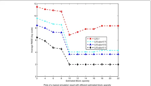
did find that any overestimatedkˆ ofkwould yield
simi-lar results. A typical simulation result is shown in Figure 1.
Therefore, for simplicity, we set kˆ = k + 1 in our
implementation.
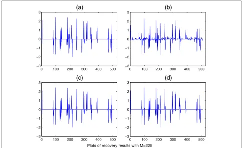
Figure 2a depicts an instance of the generated
block-sparse signal with signal length N = 512. There are
128 blocks with uneven block size and 16 active blocks
with the sparsity:k0 = x0 = 101. Figure 2b–d shows
that the recovery results by the standardlqmethod with
q = 1, the standard lq method withq = 0.5, and the
mixedl2/l1method, respectively, whenM = 225. Since
the sample size M is only around 2.2 times the signal
sparsity k0, the standardl1 method does not yield good
recovery results, whereas the mixed l2/l1 method and
the non-convexlq(q = 0.5)method achieve near perfect
recovery of the original signal. The results illustrate that if one incorporates the block-sparsity structure into the
recovery procedure, the block version of convexl1
min-imization does also reduce the number of measurement
2 4 6 8 10 12 14 16 18 20 22
0 2 4 6 8 10 12
Estimated Block−sparsity
Average RMSE (log−scale)
L2/L1 L2/Lq(q=0.7) L2/Lq(q=0.5) L2/Lq(q=0.1)
Plots of a typical simulation result with different estimated block−sparsity
0 100 200 300 400 500 −3
−2 −1 0 1 2 3
(a)
0 100 200 300 400 500
−3 −2 −1 0 1 2 3
(b)
0 100 200 300 400 500
−3 −2 −1 0 1 2
3
(c)
0 100 200 300 400 500
−3 −2 −1 0 1 2
3
(d)
Plots of recovery results with M=225
Figure 2Recovery results withM=225.(a)Original signal;(b)results withl1minimization (RMSE = 0.1301);(c)results withlq(q=0.5)
minimization (RMSE = 0.000061);(d)results withl2/l1minimization(RMSE = 0.000033).
as the standard non-convex lq minimization with some
q<1.
We further compared the recovery performance of the
standardlq method and the mixedl2/lqmethod for
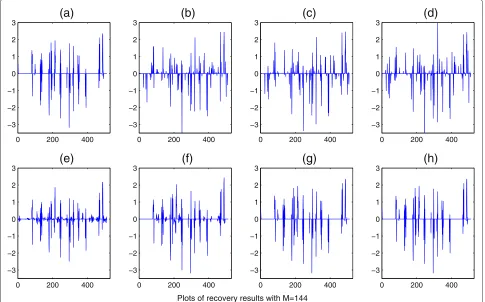
dif-ferent values of q. Figure 3 shows a similar instance as
Figure 2. We generated a block-sparse signal with the same non-zero block locations as in Figure 2a, and we
observedM = 144 measurements that is only around
1.4 times the signal sparsityk0. From Figure 3, we can see
that only the non-convexl2/lqmethod withq = 0.5, 0.1
achieve near optimal recovery results while other
meth-ods fail. The results illustrate that for anyq ≤ 0.5, the
mixedl2/lqmethod can exactly recover the original signal.
In addition, the results also demonstrate the
outperfor-mance of the non-convex mixed l2/lq(0 < q < 1)
method over the standard non-convex lq(0 < q < 1)
method.
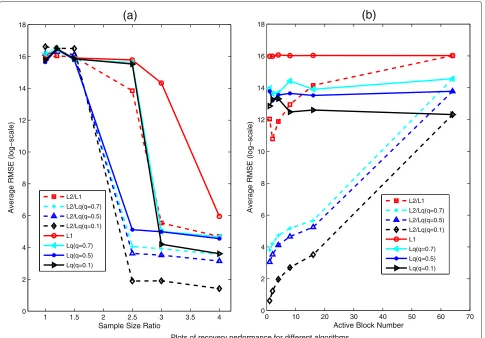
Figure 4a shows the effect of sample size, where we report the average root mean squares error (RMSE) over 100 independent random trails in the logarithmic scale for each sample size. In this case, we set signal length
N = 256, and there are 64 blocks with uneven block size
and the k = 4 active blocks were randomly extracted
from the 64 blocks. The figure indicates the decay in
recovery error as a function of sample size for all the
algo-rithms. We can observe that both the lq and the mixed
l2/lq methods improve the recovery performance as q
decreases, and for a fixedq, the mixed l2/lq method is
clearly superior to the standardlqmethod in this
block-sparse setting. To further study the effect of the active
block number k (with k0 fixed), we drew a matrix
of size 128×256 from Gaussian ensemble. We also set
the signalxwith the even block size and the total
spar-sityk0 = 64. The block size was changed while keeping
other parameters unchanged. Figure 4b shows the aver-age RMSE over 100 independent random runs in the logarithmic scale. One can easily see that the recovery
performance for the standardlq method is independent
to the active block number, while the recovery errors
for the mixedl2/lqmethod are significantly better when
the active block number k is far smaller than the total
signal sparsityk0. As expected, the performance of the
mixedl2/lqmethod becomes identical to the standardlq
method when k = k0. This illustrates that the mixed
method favors large sized block when the total sparsity
k0is fixed. Moreover, similar to the standardlqmethod,
the mixed l2/lq method performs better and better as
0 200 400 −3
−2 −1 0 1 2 3
(a)
0 200 400
−3 −2 −1 0 1 2 3
(b)
0 200 400
−3 −2 −1 0 1 2 3
(c)
0 200 400
−3 −2 −1 0 1 2 3
(d)
0 200 400
−3 −2 −1 0 1 2 3
(e)
0 200 400
−3 −2 −1 0 1 2 3
(f)
0 200 400
−3 −2 −1 0 1 2 3
(g)
0 200 400
−3 −2 −1 0 1 2 3
(h)
Plots of recovery results with M=144
Figure 3Recovery results withM=144.(a)Original signal; (b) results withlq(q=0.7)minimization (RMSE = 0.3589); (c) results withlq(q=0.5)
minimization (RMSE = 0.3857); (d) results withlq(q=0.1)minimization (RMSE = 0.4124); (e) results withl2/l1minimization (RMSE = 0.1688); (f) results withl2/lq(q=0.7)minimization (RMSE = 0.1164);(g)results withl2/lq(q=0.5)minimization (RMSE = 4.21×10⁻⁷);(h)results withl2/lq(q=0.1)
minimization (RMSE = 8.23×10⁻⁸).
7.2 Noisy recovery
In this experiment, we considered the case of recover-ing the block-sparse signals in the presence of noise. We
observed the measurementsyfrom the modely=x+z,
hereandxwere generated as the last subsection and
zwas zero-mean Gaussian noise with standard deviation
σ. In our implementation of this experiment, we setτ =
10−1max|Ty|and kept other parameters unchanged.
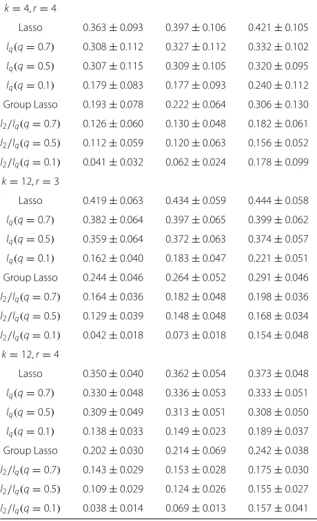
Table 1 lists the comparison results of the relative errors of the true solutions and the approximate
solu-tions yielded, respectively, by the mixed l2/lq method
and the lq method with active block numberk varying
in {4, 12}, sample sizer = M/k0 in{3, 4}, and the noise
level σ in {0.02, 0.05, 0.10}. Here, the relative errors are
defined asx−x∗2/x2. It is reported in Table 1 that
the average relative errors and the standard deviations over 100 random trails. From the table, it is seen that,
for a fixed q, the mixed l2/lq method always get better
results than the standardlqmethod. And in the low-noisy
cases (say, σ = 0.02, 0.05), as q decreases, the mixed
l2/lqmethod improves the recovery performance.
How-ever, whenσ =0.10, the mixedl2/lqmethod is not always
able to improve the recovery results whenq ≤0.7. Thus,
we may reasonably infer that there exits aq0 ≤ 0.1 such
that for anyq< q0, all thel2/lqminimization can obtain
similar recovery results when the noise level is low (σ =
0.02, 0.05); while there exits aq0≤0.7 such that asq<q0
decreases, the mixed l2/lq method is unable to improve
the recovery results whenσ =0.10.
8 Conclusion
In this article, we have investigated the block-sparse
recovery performance of the mixed l2/lq minimization
approach, especially for the non-convex case of 0 <
q < 1. Under the assumption that the measurement
matrix has the RIP with δ2k < 1/2, we have proved
that the non-convex l2/lq(0 < q < 1) method can
exactly and stably recover original block-sparse signals in noiseless case and noisy case, respectively. The suf-ficient recovery condition we obtained is weaker than
those of l2/l1 method (δ2k < 0.414), which implies
the better block-sparse recovery ability of the mixed
l2/lq(0 < q < 1) method. We have conducted a
1 1.5 2 2.5 3 3.5 4 0
2 4 6 8 10 12 14 16 18
Sample Size Ratio
Average RMSE (log−scale)
(a)
L2/L1 L2/Lq(q=0.7) L2/Lq(q=0.5) L2/Lq(q=0.1) L1 Lq(q=0.7) Lq(q=0.5) Lq(q=0.1)
0 10 20 30 40 50 60 70
0 2 4 6 8 10 12 14 16 18
Active Block Number
Average RMSE (log−scale)
(b)
L2/L1 L2/Lq(q=0.7) L2/Lq(q=0.5) L2/Lq(q=0.1) L1 Lq(q=0.7) Lq(q=0.5) Lq(q=0.1)
Plots of recovery performance for different algorithms
Figure 4Recovery performance: (a) average RMSE (log-scale) versus sample size ratioM/k0; (b) average RMSE (log-scale) versus active block numberk.
Our study so far is only concerned with the block-sparse signal recovery without overlapping blocks. While in many real applications, such as the gene expression data in bioinformatics, the blocks of elements could potentially be overlapped. Rao et al. [36] derived some tight bounds for the number of measurements required for exact and stable recovery of block-sparse signals with overlapping
blocks by the mixed l2/l1 minimization method. Their
analysis can naturally be extended to the non-convex
l2/lq(0<q<1)method. All these extensions will be part
of our future research.
Although our simulation studies in this article
demon-strate clearly that the recovery ability of the mixedl2/lq
method would be better and better asqdecreases, there
is still lack of further theoretical analysis to support for such observation. The works of [37,38] addressed the block-sparse recovery ability by an accurate analysis of the
breakdown behavior of the mixedl2/l1method. One could
then have an interest in extending these results to the case
of the mixedl2/lq(0<q<1)method as well. It is noted
that since the resultant mixed minimization problem is
Table 1 Comparison results (x−x∗2/x2) of randomly
generated signals with lengthN=256andm=64 uneven size blocks by mixedl2/lqmethod andlqmethod with four different values ofqand two different sampling sizesr=M/k0
σ=0.02 σ=0.05 σ =0.10
k=4,r=3
Lasso 0.535±0.153 0.543±0.153 0.572±0.153
lq(q=0.7) 0.467±0.184 0.458±0.177 0.504±0.209
lq(q=0.5) 0.472±0.185 0.469±0.206 0.507±0.225
lq(q=0.1) 0.355±0.243 0.364±0.251 0.461±0.253
Group Lasso 0.283±0.149 0.332±0.175 0.426±0.208
l2/lq(q=0.7) 0.159±0.125 0.189±0.173 0.312±0.268
l2/lq(q=0.5) 0.145±0.095 0.168±0.117 0.313±0.201
Table 1 Comparison results (x−x∗2/x2) of randomly
generated signals with lengthN=256andm=64 uneven size blocks by mixedl2/lqmethod andlqmethod with four different values ofqand two different sampling sizesr=M/k0(Continued)
k=4,r=4
Lasso 0.363±0.093 0.397±0.106 0.421±0.105
lq(q=0.7) 0.308±0.112 0.327±0.112 0.332±0.102
lq(q=0.5) 0.307±0.115 0.309±0.105 0.320±0.095
lq(q=0.1) 0.179±0.083 0.177±0.093 0.240±0.112
Group Lasso 0.193±0.078 0.222±0.064 0.306±0.130
l2/lq(q=0.7) 0.126±0.060 0.130±0.048 0.182±0.061
l2/lq(q=0.5) 0.112±0.059 0.120±0.063 0.156±0.052
l2/lq(q=0.1) 0.041±0.032 0.062±0.024 0.178±0.099
k=12,r=3
Lasso 0.419±0.063 0.434±0.059 0.444±0.058
lq(q=0.7) 0.382±0.064 0.397±0.065 0.399±0.062
lq(q=0.5) 0.359±0.064 0.372±0.063 0.374±0.057
lq(q=0.1) 0.162±0.040 0.183±0.047 0.221±0.051
Group Lasso 0.244±0.046 0.264±0.052 0.291±0.046
l2/lq(q=0.7) 0.164±0.036 0.182±0.048 0.198±0.036
l2/lq(q=0.5) 0.129±0.039 0.148±0.048 0.168±0.034
l2/lq(q=0.1) 0.042±0.018 0.073±0.018 0.154±0.048
k=12,r=4
Lasso 0.350±0.040 0.362±0.054 0.373±0.048
lq(q=0.7) 0.330±0.048 0.336±0.053 0.333±0.051
lq(q=0.5) 0.309±0.049 0.313±0.051 0.308±0.050
lq(q=0.1) 0.138±0.033 0.149±0.023 0.189±0.037
Group Lasso 0.202±0.030 0.214±0.069 0.242±0.038
l2/lq(q=0.7) 0.143±0.029 0.153±0.028 0.175±0.030
l2/lq(q=0.5) 0.109±0.029 0.124±0.026 0.155±0.027
l2/lq(q=0.1) 0.038±0.014 0.069±0.013 0.157±0.041
non-convex, it seems very difficult to make such similar theoretical analysis and perhaps we need more powerful tools of geometric functional analysis for the extension.
Abbreviations
CS: Compressed sensing; IHT: Iterative hard thresholding; IRLS: Iteratively Reweighted Least-Squares; NSP: Null space property; OMP: Orthogonal matching pursuit; RIP: Restricted isometry property.
Competing interests
The authors declare that they have no competing interests.
Acknowledgements
The authors would like to thank the anonymous reviewers and the Associate Editor for their valuable comments and suggestions which have helped to improve the presentation of the article. This study was supported by the National 973 Project of China under Grant no. 2013CB329404, the Natural Science Foundation of China under Grant nos. 61273020, 11001227, 11171272, and by the Fundamental Research Funds for the Central Universities (No. XDJK2010B005).
Author details
1Institute for Information and System Sciences, School of Mathematics and
Statistics, Xi’an Jiaotong University, Xi’an 710049, China.2School of
Mathematics and Statistics, Southwest University, Chongqing 400715, China.
Received: 19 August 2012 Accepted: 15 March 2013 Published: 11 April 2013
References
1. C Shannon, Communication in the presence of noise. Proc. IRE.37, 10–21 (1949)
2. A Jerri, The Shannon sampling theorem—its various extensions and applications: a tutorial review. Proc. IEEE.65(11), 1565–1596 (1977) 3. D Donoho, Compressed sensing. IEEE Trans. Inf. Theory.52(4),
1289–1306 (2006)
4. E Candes, J Romberg, T Tao, Robust uncertainty principles: exact signal reconstruction from highly incomplete frequency information. IEEE Trans. Inf. Theory.52(2), 489–509 (2006)
5. E Candes, T Tao, Near-optimal signal recovery from random projections: universal encoding strategies. IEEE Trans. Inf. Theory.52(12), 5406–5425 (2006)
6. E Candes, T Tao, Decoding by linear programming. IEEE Trans. Inf. Theory. 51(12), 4203–4215 (2005)
7. F Parvaresh, H Vikalo, S Misra, B Hassibi, Recovering sparse signals using sparse measurement matrices in compressed DNA microarrays. IEEE J. Sel. Topics Signal Process.2(3), 275–285 (2008)
8. S Erickson, C Sabatti, Empirical Bayes estimation of a sparse vector of gene expression changes. Stat. Appl. Genetics Mol. Biol.4, 22 (2005)
9. S Cotter, B Rao, Sparse channel estimation via matching pursuit with application to equalization. IEEE Trans. Commun.50(3),
374–377 (2002)
10. D Malioutov, M Cetin, A Willsky, Sparse signal reconstruction perspective for source localization with sensor arrays. IEEE Trans. Signal Process. 53(8), 3010–3022 (2005)
11. Y Liu, Q Wan, Enhanced compressive wideband frequency spectrum sensing for dynamic spectrum access. EURASIP J. Adv. Signal Process. 2012(177), 1–11 (2012)
12. A Majumdar, R Ward, Compressed sensing of color images. Signal Process.90(12), 3122–3127 (2010)
13. J Huang, T Zhang, The benefit of group sparsity. Ann. Stat. 38(4), 1978–2004 (2010)
14. Y Eldar, M Mishali, Robust recovery of signals from a structured union of subspaces. IEEE Trans. Inf. Theory.55(11), 5302–5316 (2009)
15. M Stojnic, F Parvaresh, B Hassibi, On the reconstruction of block-sparse signals with an optimal number of measurements. IEEE Trans. Signal Process.57(8), 3075–3085 (2009)
16. R Baraniuk, V Cevher, M Duarte, C Hegde, Model-based compressive sensing. IEEE Trans. Inf. Theory.56(4), 1982–2001 (2010)
17. Y Eldar, P Kuppinger, H Bolcskei, Block-sparse signals: uncertainty relations and efficient recovery. IEEE Trans. Signal Process.58(6), 3042–3054 (2010) 18. Z Ben-Haim, Y Eldar, Near-oracle performance of greedy block-sparse
estimation techniques from noisy measurements. IEEE J. Sel. Topics Signal Process.5(5), 1032–1047 (2011)
19. A Majumdar, R Ward, Fast group sparse classification. IEEE Can. J. Electr. Comput. Eng.34(4), 136–144 (2009)
20. S Foucart, M Lai, Sparsest solutions of underdetermined linear systems via
lq-minimization for0<q≤1. Appl. Comput. Harmonic Anal. 26(3), 395–407 (2009)
21. R Chartrand, V Staneva, Restricted isometry properties and nonconvex compressive sensing. Inverse Problems.24(03520), 1–14 (2008) 22. R Saab, R Chartrand, O Yilmaz, inIEEE International Conference on Acoustics,
Speech and Signal Processing,. Stable sparse approximations via nonconvex optimization (IEEE, 2008), pp. 3885–3888
23. R Chartrand, Exact reconstruction of sparse signals via nonconvex minimization. IEEE Signal Process. Lett.14(10), 707–710 (2007) 24. Z Xu, H Zhang, Y Wang, X Chang, Y Liang,l1/2regularization. Sci. China
Inf. Sci.53(6), 1159–1169 (2010)
25. Z Xu, H Guo, Y Wang, H Zhang, The representative ofl1/2regularization
26. Z Xu, X Chang, F Xu, H Zhang,L1/2regularization: a thresholding
representation theory and a fast solver. IEEE Trans. Neural Netw. Learn. Syst.23(7), 1013–1027 (2012)
27. Q Sun, Recovery of sparsest signals vialq-minimization. Appl. Comput. Harmonic Anal.32, 329–341 (2012)
28. M Lai, Y Xu, W Yin, Improved iteratively reweighted least squares for unconstrained smoothedlqminimization. SIAM J. Numer. Anal. (2013). [http://www.math.uga.edu/~mjlai/papers/LXY2013.pdf]
29. E Candes, The restricted isometry property and its implications for compressed sensing. Comptes Rendus Mathematique.346(9–10), 589–592 (2008)
30. S Chen, D Donoho, M Saunders, Atomic decomposition by basis pursuit. SIAM J. Sci. Comput.20, 33–61 (1998)
31. M Yuan, Y Lin, Model selection and estimation in regression with grouped variables. J. R. Stat. Soc.: Series B (Statistical Methodology).68, 49–67 (2006) 32. M Fornasier, H Rauhut, Recovery algorithms for vector-valued data with
joint sparsity constraint. SIAM J. Numer. Anal.46(2), 577–613 (2009) 33. I Daubechies, R DeVore, M Fornasier, C Güntürk, Iteratively reweighted
least squares minimization for sparse recovery. Commun. Pure Appl. Math.63, 1–38 (2010)
34. A Aldroubi, X Chen, A Powell, inProceedings of SampTA. Stability and robustness of lq minimization using null space property (Singapore, 2011) 35. M Lai, L Liu, A new estimate of restricted isometry constants for sparse
solutions (2011). http://www.math.uga.edu/~mjlai/papers/LaiLiu11.pdf 36. N Rao, B Recht, R Nowak, Tight measurement bounds for exact recovery
of structured sparse signals. Arxiv preprint arXiv.1106, 4355 (2011) 37. M Stojnic,l2/l1-optimization in block-sparse compressed sensing and its
strong thresholds. IEEE J. Sel. Topics Signal Process.4(2), 350–357 (2010) 38. M Stojnic, Block-length dependent thresholds in block-sparse
compressed sensing. Arxiv preprint arXiv.0907, 3679 (2009)
doi:10.1186/1687-6180-2013-76
Cite this article as:Wanget al.:On recovery of block-sparse signals via mixedl2/lq(0<q≤1)norm minimization.EURASIP Journal on Advances in Signal Processing20132013:76.
Submit your manuscript to a
journal and benefi t from:
7Convenient online submission
7Rigorous peer review
7Immediate publication on acceptance
7Open access: articles freely available online
7High visibility within the fi eld
7Retaining the copyright to your article