R E S E A R C H
Open Access
Fast, parallel implementation of particle
filtering on the GPU architecture
Anna Gelencsér-Horváth
*, Gábor János Tornai, András Horváth and György Cserey
Abstract
In this paper, we introduce a modified cellular particle filter (CPF) which we mapped on a graphics processing unit (GPU) architecture. We developed this filter adaptation using a state-of-the art CPF technique. Mapping this filter realization on a highly parallel architecture entailed a shift in the logical representation of the particles. In this process, the original two-dimensional organization is reordered as a one-dimensional ring topology. We proposed a
proof-of-concept measurement on two models with an NVIDIA Fermi architecture GPU. This design achieved a 411-μs kernel time per state and a 77-ms global running time for all states for 16,384 particles with a 256 neighbourhood size on a sequence of 24 states for a bearing-only tracking model. For a commonly used benchmark model at the same configuration, we achieved a 266-μs kernel time per state and a 124-ms global running time for all 100 states. Kernel time includes random number generation on the GPU withcurand. These results attest to the effective and fast use of the particle filter in high-dimensional, real-time applications.
Introduction
In applications in the field of image processing [1,2], nav-igation [3], and financial mathematics [4,5] we deal with non-linear state-space models subject to additive noise which is not restricted to Gaussian noise. Even if each state only depends on the previous state (i.e. the sequence follows the Markov dynamics [6]), a Kalman filter [7] is suboptimal for the state estimation due to non-linearity and non-Gaussian noise. Furthermore, an analytic solu-tion is often not available. In contrast, sequential Monte Carlo methods (SMCM) offer a probabilistic framework that is suited to non-linear and non-Gaussian state-space models. In our work, we focus on a particle filter (PF) [8] which is both part of the SMCM algorithm family and can be considered an extension of a Kalman filter. Our main aim is to introduce a fast and reliable PF on a GPU.
We restrict ourselves to particle filters which use sequential importance resampling (SIR) [9]. The PF algo-rithm (as described in the next section in detail) has a high running time due to the resampling step - according to the complete cumulative distribution; therefore, an adequate parallel implementation would fetch a remark-able speed-up. The classical resampling algorithm of
*Correspondence: [email protected]
Faculty of Information Technology, Pázmány Péter Catholic University, Práter str. 50/a, Budapest H-1083, Hungary
this process needs N processors to reduce its computa-tional need from O(N) to O(log(N)), and so, this par-ticle filter was considered unsuitable for parallelism. It should be noted that this statement holds as long as the the complete cumulative distribution is required for any particle.
Whilst the price of a device is relatively low, graph-ics processing units (GPUs) have a high computational efficiency. Therefore, GPUs represent an attractive imple-mentation platform. Since GPUs are spreading fast, thanks to the game industry, and developing rapidly, com-putational effort is still increasing by leaps and bounds.
There have been some former implementations to par-allel architectures [10-19]. In [11], an implementation strategy is proposed which is parallel; however, it cannot maintain the local connections of the particles. The par-ticles are split into smaller groups (around 100 parpar-ticles) which perform operations independently. The informa-tion exchange among the particle groups is occasional; share ratio is suggested at around 25%. Researchers admit that the reduced flow of information of the distributed particle filter degrades the quality of estimation compared to the original algorithm which resamples according to the complete cumulative distribution.
Besides continuous information sharing, random num-ber generation has a significant effect on the filter result.
The simple solution is creating random numbers on the CPU using any of the many implemented reliable random libraries proposed in [10]. However, these researchers are aware of the great disadvantage of this technique, mainly the huge delay raised by data transfer. Hence, they prefer a sufficient GPU random sequence generator instead.
In the resampling step, each particle requires infor-mation from all other particles. This adds a high computational delay. Resampling is based on the rela-tive importance of the particles, but the technique is not restricted to uniform sweepstake over the weights (systematic resampling).
Metropolis resampler [20] in each resampling step iter-atively selects B times a candidate according to a given rule for each particle. Since the aforementioned rule is based on pairwise operations, the efficient mapping on many-core architecture is realizable as follows.
For eachp∈ 1,. . .,Nparticle in eachi∈ 1,. . .,B iter-ation, two main parameters,aipandsip, are used, whereaip stands for the actual particle andsipstands for the selected particle;aipis initialized with particlep. With uniform dis-tribution, we draw auiprandom number on [ 0, 1)andsip particle from the complete particle set. If the ratio of the
weights
w sip
waip is overuip, the selected particle is indicated
as actual. This pairwise operation can be performed inde-pendently; therefore, efficient implementation is possible on parallel architecture.
Resampling can also be accelerated if the number of par-ticles is decreased. However, there is a trade-off between particle number and estimation accuracy. The spreading-narrowing technique in [12] proposes a solution. A toler-ableNnumber ofbasis particlesgenerates anN×Plarge set by propagating each particle based on the system tran-sition model for a sequence ofPstates. EachPisubset then
delivers a single particle based on alocal particle selection process. It either uses maximizing importance selection (MIS), taking the highest weighted particle, or it uses sys-tematic resampling (SR) on the weights. SR has a lower complexity than a global resampling on anN×Psize set as P takes values from{10, 20, 50, 100, 200, 500} based on the current application, and for eachPi set, it can be
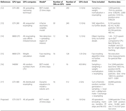
performed parallel to each other. While MIS has an even lower complexity, it is more sensible to the noise intro-duced by the artificial propagative spread of the particles. For the measurements, they used a bearing-only tracking (BOT) model with 25 time steps; therefore, we can make direct comparison for the estimation error. For [12], the position error is in the range of 0.06245 to 0.06226, which is slightly lower than our error, but still the same range. Execution time, which is the sum of sampling, weight normalization and resampling times in [12], and total run-time in our work (including memory transfers, file I/O, etc.), shall be compared to our proposed algorithm with
regard to the different devices, which still indicates that our technique is faster (see Table 1).
We investigated [13-15] from CUDA ZONE, which also addresses particle filteringon GPU or parallel and GPU. In [15], only the weight calculation is performed on the GPU as the focus of this paper is not particle filtering. However, this work is slightly out of our scope as the aim was the fast estimation of face tracking with PF; the contribution of parallelism on the GPU is relevant in the total speed-up. Three different case studies are presented for Monte Carlo methods in [13]. They found out that global resampling has a significant influence on the runtime, and they achieved 10 to 37 times speed-up compared to a single threaded CPU implementation. The measurements were made with the use of a factor stochastic volatility model; therefore, direct comparison to our benchmark model is troublesome. However the computations run on the GPU, the resampling - unlike in our proposed work - is not parallel but sequential. In [14], resampling is performed with a technique based on using an offline-created and offline-uploaded texture of uniformly distributed random numbers. The focus of [14] was single- and multiple-object tracking, using skin detec-tion and spreading the region of interest; therefore, the lack of common model encumbers the direct comparison of the result to our proposed method.
Table 1 Highlighted related works
References GPU type GPU computes Modela Number of SMs on GPU
Number of cores
GPU clock Time included Runtime data
[12] GTX 280 All; spreading-narrowing technique
BOT model, 25 time steps
30 240 1.3 GHz Sampling +
weight [13] GTX 280 All; sequential
resampling
A factor stochastic volatility model
30 240 1.3 GHz SMC algorithm:
no further details [14] 8800 GTS All; resampling
uses
offline-12 96 1.2 GHz Object tracking
time; no further
16 128 1.35 GHz Face tracking
algorithm time; [17] GTX 580 All; distributed
resampling
Dynamic equations to model a robotic arm
16 512 2 GHz Sum of kernels:
random number
Proposed GTX 550 Ti All; all parallel BOT model, 24 time steps
4 192 1.8 GHz All operations
(including mem-cles 77 ms 0.07 posi-tion error
Summary of related works including the following parameters: used model, outline of the technique and the GPU if measurements were made on it. Direct comparison is often hardly feasible due to the differences of the mentioned parameters.aAs given in the references;bframes per second.
information share among the subsets. Central estima-tion is calculated using the results of subsets. In [19], three different techniques are presented, and locally dis-tributed particle filter is considered as giving the best speed-up and estimation. Also, this is the closest from the three presented methods to our approach; however, operations are performed without any information share and only simulation results are given for a discrete time non-linear dynamic model of nearly constant turn. For the summary of related work, please see Table 1 where we highlighted the most relevant GPU-related works. The table also reveals the difficulty of direct comparison of the results due to the different models, data and GPU devices.
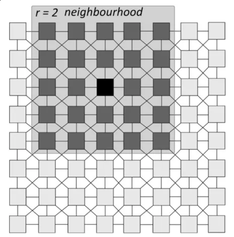
We can say that resampling is a key point in SIR parti-cle filtering. Approaches to deal with SIR resampling try to optimize the speed quality trade-off for the given set-up. Cellular particle filter(CPF) [21] introduces a third approach for the resampling problem by changing the logic representation of PF to a two-dimensional (2D), locally connected grid inspired by cellular neural network (CNN) architecture [22]. Each element in the grid is con-nected to each of its eight neighbours enabling rapid local information flow. The critical resampling step can then be performed on a subset in anrradius neighbourhood.
dimension of resampling sets, CPF offers a solution for the problem of reduced local information change, which is stated in [11]. However, this representation is not opti-mal for a GPU architecture. Hence, we made some fur-ther modifications to achieve an efficient implementation which exploits the characteristics of GPUs. Besides, one of our principles is to generate random sequences on the GPU since NVIDIA SDK Mersenne Twister proved to be insufficient at low numbers. Therefore, we explored possi-ble solutions and finally propose two different approaches for random number generation.
This paper is organized as follows: the ‘Background and theory’ section describes the necessary background and theory for hidden Markov models (HMMs), particle fil-ters, especially cellular particle filter, and architectural perspectives. In the ‘Our proposed method’ section, we introduce our proposed method in detail. The ‘Evaluation and results’ section provides information about applied measurement techniques and our results. Finally, The ‘Conclusions’ section delivers our conclusion.
Background and theory
Hidden Markov models and particle filtering
HMMs consist of two stochastic processes. One of them is the trajectory of hidden statesxtaccording tot=0, 1,. . .,
determined by Markov dynamics:
xt+1=ϕ(xt,e1(t+1)) (1)
The other contains observations yt, for t = 1, 2,. . .,
depending only on the current hidden state plus an addi-tive noise which is not limited to Gaussian:
yt=ψ (xt)+e2(t) (2)
These notable extensions transfer the resolution beyond the Kalman filter [7] to the scope of particle filtering. In case of state estimation, it is considered thatϕ,ψ, func-tions and distribufunc-tions of e1(t) ande2(t) are given. For more information about hidden Markov models, see [6].
A particle filter is a tool for estimating the hidden states based on the observation. It is not an analytical calculation but the use of a set of particles at each time step that fol-lows the model dynamics. The algorithm is built up from three main steps in each timet(i.e.state).
The first step is error calculation which assigns each particle a fitness value. It is performed between the cur-rent particle value and the curcur-rent observation value (same for all particles at a time step) as described in Equation 3. L stands for the likelihood value, for each i = 1,. . .,N particle, andlis the density function of the noise of the hidden process (e1(t)):
Lit = l(yt − ψ (x)) (3)
Each particle weight is set based on this likelihood:
wit = Lit (4)
where Lit is the fitness value of theith particle, and for simplicity in resampling, each weight is normalized:
wit = w
The second main step is resampling. While there are many alternations, we focus on a particle filter with sequential importance resampling [23]. We choose a new ξ particle set from our current particles, ξi = ξη(Ui),
where η(Ui) stands for the uniform random
sweep-stake, using the set of corresponding normalized particle weightswt(see Figure 1 and Equation 6, for particlesi,j=
1,. . .,N):
P(η(Ui)=j)=wtj (6)
The resampled setξtis used for the current estimation (e.g. taking the mean). The last main step of the loop is the iteration, which is identical to sampling at the beginning of the loop. In this last step, we use the model to generate the next time step’s initial particle set using the model:
ξti+1=ϕ(ξti,e1(t+1)) (7)
whereξtiare the resampled particles,i= 1,. . .,N. Parti-cle filtering technique has been used since 1962 [24], and SIR particle filter has been used since 1993 [23]. Still, the proof of convergence was published only 18 years later [25]. More information about particle filters can be found in [23,26]. Henceforward, ‘original algorithm’ stands for the algorithm described in this section.
Cellular particle filter
In the resampling step, for each retake, we have to use the whole particle set. This is highly time-consuming and for a long time was considered not parallelizable. Cellular par-ticle filter [21] offers a solution for this problem, and in contrast to other distributed particle filters [11], it main-tains local connectivity, which allows for each particle to access the information of its neighbours in each time t. This ensures the same or, at some parameters, even bet-ter quality of approximation. To provide theoretical proofs for our concept is beyond this articles’ scope, but see [21] for some experimental validation.
The main idea lies in the logical representation. The set of particles are organized in a CNN-inspired architecture,
namely, a locally connected two-dimensional grid with uniform elements where each element is only connected to its eight neighbours. Based on the connections, we can define a neighbourhood for celli(ie. cellCi,j) with radius
r: Ck,l ∈ Ni if k ∈[i− r,i +r] and l ∈[j− r,j+ r]
(see Figure 2).
We can retrace the original algorithm if we set the neighbourhood size for each particle to fit the dimension of the grid. However, if we set a smallerrradius, it defines a locally connectedNineighbourhood for eachiparticle:
Wti =
j∈Ni
Ljt (8)
Using the sum of weightsWtiof the neighbourhood, in this case, the weights are set to
wjt(i) = L
j t
Wti (9)
wherej∈Ni.
Now, the resampling step can be performed for each i particle simultaneously within the localNi
neighbour-hood according to the local distribution of the weights. Fetching the weights is realized by local communication on the physical device, therefore, it is fast. The ran-dom take on all subsets around eachiparticle produces
N resampled particles, respectively. Hence, the
time-consuming part is parallelized, and the required compu-tational effort is essentially independent of the number of particles. This method might seem to be similar to
Figure 2CNN architecture.CNN processor array architecture: two-dimensional fully connected grids. The light gray background highlights ther=2 size neighbourhood around the black cell.
distributed particle filters [11], but there are no commu-nication limits among the subsets in any time states.
CPF is suited to GPU architecture due to its parallel, locally connected nature. Our aim is to ensure efficient computation and therefore to exploit the properties of the GPU in our adaptation.
GPU details
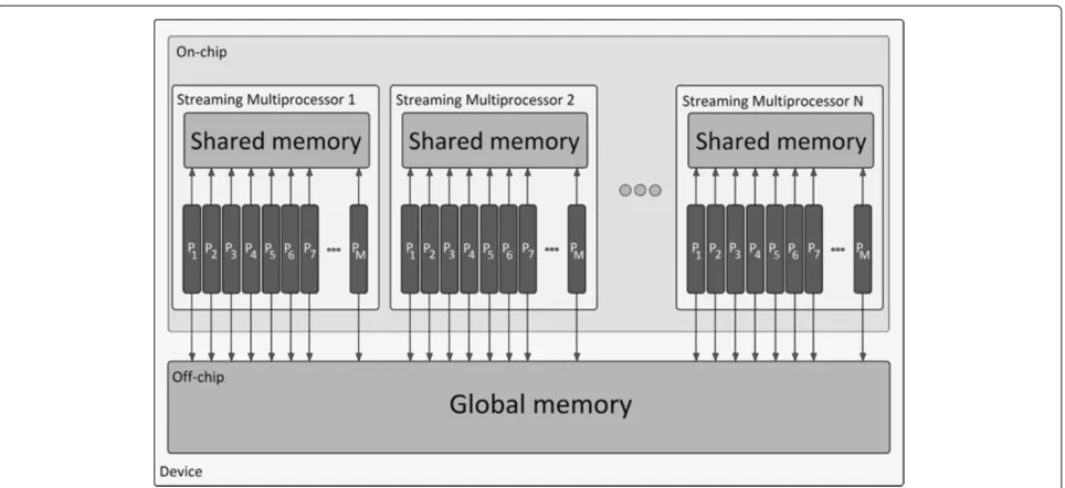
Our proposed mapping is based on the GPU features summarized in this section. We used NVIDIA CUDA (see [27]) for notations and details. Figure 3 shows the basic architecture of the GPU considered mainly from the view of mapping CPF to this architecture.
In the logical sense, the kernel function is the function executed on the device. It is executed simultaneously by threads. Threads are organized into blocks (typically 32 to 512 in each, based on the current task), in a one-, two-, or three-dimensional array. Blocks are organized in a grid in a one- or two-dimensional array. The number of threads per block and block per grid is called execution configuration.
In the physical sense, the device is built up from stream-ing multiprocessors (SMP). Each SMP consists of an SD RAM, a number of cuda cores and a scheduling unit. The SD RAM is an on-chip memory, with a few tens of clock cycle delays, its size is 64 kB, and it is divided to L1 cache and shared memory. The GPU has an off-chip global memory to be accessed by each SMP. Its size is usually around 1 to 4 GB, depending on the type of the particular device. Its delay is 400 to 600 clock cycles. Addi-tionally, there are two other types of memory spaces that both reside off-chip and are cached on-chip. The first one is texture memory, and the second one is constant memory. The latter’s size is 64 kB.
Blocks are mapped to SMPs. Shared memory of block Bi can only be accessed by the threads which reside in
Bi. The communication and data share among the blocks
Figure 3GPU architecture.Simplified architecture of the GPU. Streaming multiprocessors (SMP) contain cuda cores (Pi), an on-chip (shared), fast memory, scheduling unit and special function unit. Besides, all cuda cores in all SMPs have access to the large and slow off-chip memory (global memory).
To achieve a high throughput, on-chip memory (shared memory) should be used if threads require frequent data access. Therefore, the main computational tasks are per-formed block-wise, in the shared memory of the blocks, and only necessary global synchronization is performed through global memory. Although the two-dimensional texture and surface memory would also be feasible, shared memory throughput can be optimized for a one-dimensional array type representation; thus, structural aspects in CPF algorithm were reconsidered.
In the shared memory, we use arrays with the size 512 for the particles, the error terms, the normalizing sums and the uniform random numbers. In our case study, when taking the highest neighbourhood size and at a single precision 10,250 bytes are occupied. Each shared memory can access a 48-kB memory/multiprocessor at compute capability 2.x [27]. Global memory in recent GPUs is at least 1 GB which restricts the number of states in the observation and estimation, but both memory access is high enough for our computations.
Our proposed method
Random number generation
The SIR in each t time step requires the same amount
of random numbers as the number of particles. We intend to generate these random sequences on the GPU device instead of the CPU to spare repetitive data trans-fer between the main memory of the system and the global memory of the device as recognized in [10]. The distribution of the random numbers in the resampling is
critical on the quality of the estimation. If it is not uni-form, though the drawing of particles should depend on the weights exclusively, then it would be biased.
Recently GPU random number generation for various purposes has become widely investigated and well tested (see [29-31]). NVIDIA provides two solutions for random number generation. The first option was the Mersenne Twister in the SDK. Unfortunately, we observed that the generated distribution is inappropriate for a small set (hundreds or thousands) of numbers and is primarily admissible for around two million numbers and above. We made delicate modifications to get admissible distribution (see Appendix for details). The second option wascurand, which proved to be fast and appropriate.
GPU CPF algorithm
Figure 4Ring type topology.Restructuring linear representation of
Nblocks to a ring type topology.Bistands for theith block, andNBi
for the corresponding neighbourhood from the previous block,
i∈1,. . .,N.
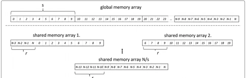
The local connectivity is preserved by choosing each shared memory array size higher than the thread number exactly with the size of the required neighbourhood. Each thread with indexican obtain itskneighbours at indexes i−1,i−2,. . .,i−k.
In the following, we specify some implementation details. Although the operations are mainly performed in the shared memory because of the synchronization and CPU-GPU data transfer, the following variables are global memory arrays: the observation sequence (Y), the state estimation (X) and the set of particlesxparticles. The number of particles is denoted byN.Y is naturally given, Xis empty, andxparticles is initialized withN samples of
the same distribution asntdescribed in Equation 10. The
number of threads in a block was set to 256. The size of the neighbourhood isr, meaning each particle is connected to exactlyr+1 particle (every particle is connected to itself ).
In each block, two shared memory arrays of size 256+rare created for particle statesxsharedand fitness valuesLshared; additionally, two arrays whose size equal the number of threads in a block are allocated for uniform
pseudo-random numbers Ushared and normalizing weights
wshared.
In each time step, we copy the particle values from the global memory to the shared memory by overlap-ping split (see Figure 5 for illustration). We load 256 values respectively to each shared memory to the parti-cle’s array (xshared) but sparing its firstrelements. These positions are filled with the r neighbours in the global memory of the first element inxshared. For the very first element, we use a circular approach by taking the val-ues from the end of the global memory array. There are three kernel calls for each estimated values to provide full synchronization.
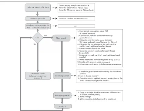
The main kernel performs the following operations in each time stept (also see Figure 6 with the same num-bering), where global and local thread IDs are defined as follows:igl = blockDim.x×blockSize.x+threadId.x and iloc = threadId.x, where threadId.x is the thread index in the thread block,blockSize.x is the number of
thread per each block, and blockDim.x is the index of
the block. For more information about the terminology, see [27]:
I Initialization:
2. xshared[iloc+r]←xparticles[igl].
2. Ifiloc<r, then
xshared[iloc]←xparticles[igl−r+iloc]. 2. Ifigl<r, then
xshared[iloc]←xparticles[N−r+igl].
Figure 6Overview.Flowchart of our implementation on the GPU device.Sdenotes the number of threads in each block,xparticlectdenotes the
resampled particle set intstate. The observation sequence consists aboutTstates.
II Error calculation:
3. Lshared[iloc+r]←l(Y[t]−xshared[iloc+r]).
3. Ifiloc<r, then
Lshared[iloc]←l(Y[t]−xs[iloc]).
4. wshared[iloc]←
Lshared[iloc]+ · · · +Lshared[iloc+r]get
normalization sums for each particle.
III Resampling:
5. Ifiloc==0, refresh seed value of the block.
6. FillUsharedwith uniform random numbers.
7. Iteratively sumLshared[jloc]/wshared[jloc] wherejloc=iloc,iloc−1,· · ·,iloc−r. Stop if adding anLshared[kloc]/wshared[kloc]term affects the sum to exceedUshared[iloc]for the first time.
8. From the neighbourhood ofiloc, the
correspondingk particle is selected to
xparticlest[iloc]. Estimation is calculated from
these particle values.
IV Iteration on particles (generating samples for next state):
9. FillUsharedwith normally distributed random
numbers.
9. xshared[r+iloc]←ϕ(xshared[r+iloc] ,nt).
10. xparticles[igl]←xshared[iloc+r].
The estimation is performed by two kernel calls. The first kernel calculates the sum for each shared memory xparticlest arrays to a global memory arraygSum. The
sec-ond kernel takes the average value of gSum with respect to the number of particles.
shared memory to spare time; (2) the number ofif state-ments is minimized as possible and are transformed to ternary expressions; and (3) the shared memory arrays are reused; therefore, even some parameter passes can be spared.
Evaluation and results
Model
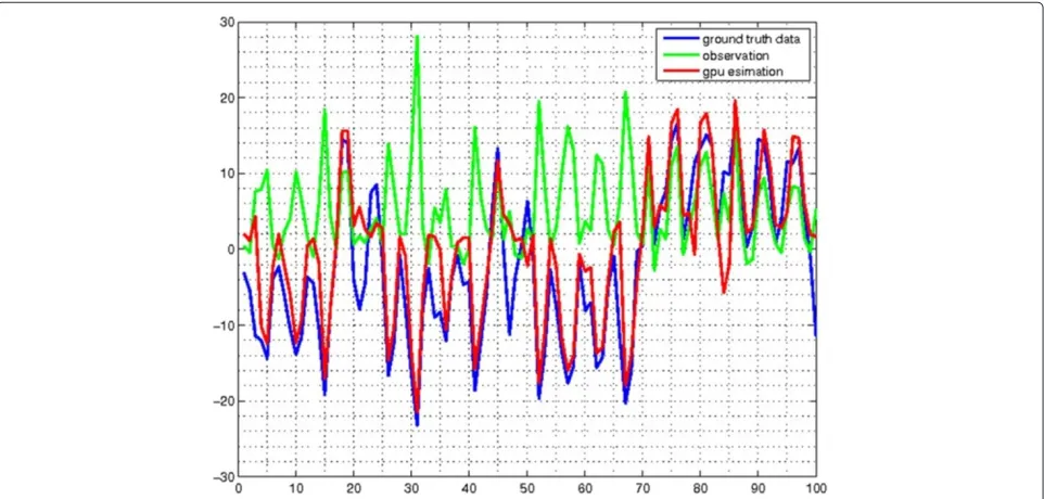
The implemented algorithm was tested on two different widely used models. The first was the following bench-mark model [8,23,32,33]:
xt+1= xt
2 +
25xt
1+x2t +8 cos(1.2t)+nt (10)
yt=
x2t
20+ut (11)
This model is non-autonomous, non-linear and has a continuous state space; thus, linear tools for state esti-mation are not applicable. The state of the system isxt,
and the observation is yt; nt and ut are IID Gaussian
sequences,nt ∼ N(0, 10)andut ∼ N(0, 1).
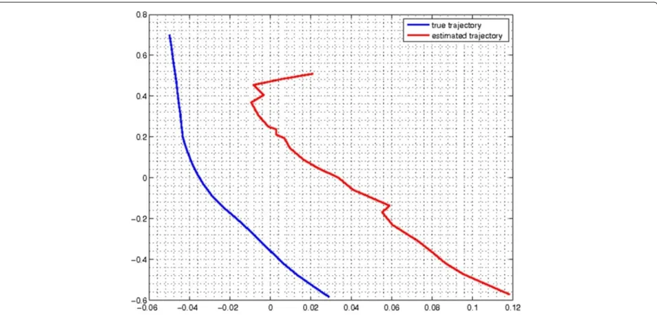
The second model was a bearings-only tracking (BOT) model originally presented in [23] and also analyzed in [16,17]. For the illustration about the trajectories of each model, see Figures 7 and 8.
Measurements
There are two aspects of the measurements, namely, the average quality and the required time for one estima-tion. These two quantities were monitored with different
configurations (number of particles and radius of neigh-bourhood) of the filter. The number of particles were swept through the following values: 2,048, 4,096, 8,192, and 16,384, while the radius of neighbourhood took the following values: 32, 64, 128, and 256. Consequently, 24 pairs of these are composed; in our terminology, these are called configurations (i.e.N,rpairs). For the first model, the input observation trajectories (yt) during the tests
were exactly the same as the ones used in [21] to ensure a fair comparison. For the BOT model, we generated 100 trajectories over 24 time steps based on the given state transition equations in [23] and, respectively, the observations.
Measurements were done on a PC with Intel i5-660 (3.33 GHz, 4-MB cache) 4 CPU with 4-GB system mem-ory running Ubuntu Linux 11.04 with kernel version 2.6.38-15 (amd64). We used an NVIDIA GeForce GTX 550 Ti GPU with 1-GB GDDR memory with CUDA toolkit 4.1 with 295.49 driver version. The following nvcc compiler options were used to drive the GPU binary code generation: -arch=sm_20;-use_fast_math. We also made some measurements with -arch=sm_13. The host c code was compiled with gcc 4.5; the compiler flag was -O2. GPU kernel running times were mea-sured with the official profiler provided by the toolkit, and the global times were measured by the OS’s own timer. The kernel time measurements include the par-ticle filtering kernel of a single time step; the global times include all operations during the execution for all states (file I/O, memory allocations, computational operations, etc.).
Figure 8Trajectory for the BOT model.The positions (x−y) are the hidden states (blue), the estimation from the GPU CPF is red. The mean of the position error is about 0.08.
The quality of estimation was measured by the mean square error (MSE). In the case as the first model, 1,000 estimations for each configuration of 100 time step long HMMs were made. In the case of the BOT model, the generated 100 trajectories were estimated with each configuration.
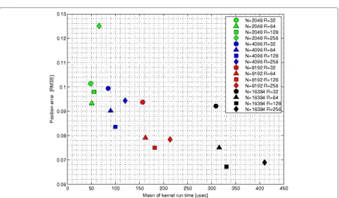
Estimation quality
The quality of estimation for the first model was mea-sured by the MSE between each hidden and estimated trajectories, for the BOT model by the position error (ie. Euclidean distance). We used 1,000 and 100 differ-ent state sequences (i.e. observation sequences) for each configuration in the first model and the BOT model, respectively.
Figure 9 presents the quality of estimation for the first model; Figure 10, for the BOT model, namely the mea-surement error with respect to the meamea-surement time. Each point represents a configuration since its x andy coordinate values are the mean of 1,000 and 100 execu-tions for the two models, respectively. For the first model, it can be seen that using more than 4,096 particles slightly improves the quality of estimation.
However, for the BOT model estimations, where the particle number is more or equal to 2,048 (alike [16,17]), provide a fair result. The position error is in the same range as in [17] and our proposed method. The results suggest that the proportion of the neighbourhood size to the particle number realizes an information sharing ratio among the particles. This can be seen in Figure 10: the optimal ratio for the configuration is when the position
error is minimal, typically marked with squares except 2,048 particles when marked with triangle.
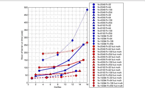
Time
Figure 11 presents the total runtime of the kernels in the first model. The blue lines represent the running times with compiler option -arch=sm_13; the red lines, with -arch=sm_20;fast_math;. The first compilation set-ting will be referred to as old target code; the latter, as new target code. It can be seen that for the neighbourhood size below 64, the old target code performs 20% faster than the new. With the new target code, we can achieve a 40% to 45% improvement in execution time if the old target code is considered as 100%.
Due to the logic of physical mapping of blocks to mul-tiprocessors, the GPU is under-utilized for particle num-bers under 2,048. Above this particle number, the scaling of the execution time is nicely illustrated in Figure 11.
For various neighbourhood sizes, we can say that the required time is proportionally increasing to the number ofR. This phenomenon is due to the resampling step as it examines the candidates sequentially for resampling. Even if the proper particle is found, the loop does not termi-nate until the current particle is compared to all of its neighbours to avoid warp desynchronization.
Figure 9Estimation quality for the first model.This figure shows the mean square error of the estimation as a function of kernel times. It can be seen that at a given particle number with the increase of the neighbourhood size, the estimation quality improves simultaneously.
Figure 11Kernel runtimes with different nvcc flags.This figure shows the difference between the total running times for the different compiler options for the first model. The use of fast math and sm_20 has a significant effect on the kernel times.
time measurements include. For the first model, see total execution times with and without host code optimization (made by compiler) in Figure 12.
Discussion
A key point of our proposed algorithm is the local resam-pling technique which has a high influence on the esti-mation quality. This key point can be viewed as diffusion of information inasmuch as every particle with relatively high likelihood attracts all particles which has this likely particle in its neighbourhood. In this way, the other par-ticles not having this very particle in their neighbour-hood are not affected in this state estimation time step. Although it is not the traditional full resampling, it enables the algorithm to be sufficient even at high-uncertainty dynamic models. The BOT model is not a highly uncertain model as sharp changes are unlikely, but in the one dimen-sion benchmark model (as you can see in Figure 7), rapid and significant changes are typical. Cellular resampling preserves the diversity of the particles to avoid quality loss. The estimation error for a given particle number changes within a narrow range around the optimal, depending on the neighbourhood size. This modulation is not in direct or inverse ratio to the number of used neighbours but fol-lows a descending and then increasing characteristic (like the shape of letter ‘U’, see Figure 10). This indicates that
for a given model, at any particle number, there exists an optimal share ratio range among particles to achieve the lowest error. In our proposed method, the information sharing ratio is tunable and may be modulated adaptively; therefore, it broadens the range of options than using a predefined information share value. For further details and reasoning, see [21].
Figure 12Global runtimes for the first model with and without O2.This figure shows the speed-up of the host code optimization compiler option for the first model.
from the global memory to the shared memory), and the access time of the constant cache is similar to the access time of the shared memory.
Two different models were used in this work. The first one is a synthetic benchmark model. It does not model any physical system of practical interest. It is just a widely used highly non-linear model since both the observation and the state transition is non-linear, unlike the other model (BOT model) which has a linear state transition. This second model describes a bearing-only tracking of an object in the two-dimensional (x−y) plane, with a fixed observer position, where observation (z) is the bearing of the object trajectory. Through the BOT model, we can compare the estimation quality of CPF to GPU particle fil-ters in [11,16,17]. We can see that the error is in the same range with [16] and is better than error in [11]. According to the error and time measurements, we can state that this is a feasible mapping from a virtual machine (CNN UM-inspired architecture) to a state-of-the-art architecture with a mature ecosystem available at a low cost.
In this algorithm, each thread executes roughly 300 to 2,100 floating point operations. This depends on the neighbourhood size. Those operations which are performed through the neighbourhood are additions and unfortunately divisions (calculating the actual weights
with the norming sums in the resampling). This amount of divisions are clearly one bottleneck. The speed-up achieved withfast_math also supports this explanation. The other bottleneck of the algorithm is the shared mem-ory size and access pattern. If more threads could reside in a block, then the ratio of the overlay among blocks due to the neighbourhood size would be less. In the resampling, branches are unavoidable, and fork and join of threads within a warp are necessary. There are a number of for-loopswhich iterate through the given number of iterations where the end index is unknown at the time of host code compilation. In our framework, it is only known in run-time. Still, for a given application, optimal parameters can be set directly in the code based on measurements, and therefore, loop unroll can be applied. Another approach can be just-in-time (JIT) kernel compilation. This method is effective only if the JIT compilation time is less than the cumulative gain from the loop unrolling through the state predictions.
as the threads are independent from each other, not count-ing the synchronization points. However, on GTX 550, the time increase starts after 1,536 threads (on 6 SMPs× 256 threads). On GTX 580, there are 16 multiproces-sors in comparison with the 6 multiprocesmultiproces-sors of GTX 550; therefore, under 4,096 threads, the GPU would be under-utilized (i.e. GTX 580 is the top GPU of the Fermi GPUs).
A direct comparison to a CPU, sequential particle fil-ter, is not entirely adequate; still, we would like to mention differences in the running time. In [21], particle filter was realized and used as a reference for time measurements of the proposed algorithm; therefore, we compare our results to this also. However, time measurements are not pre-sented for many particle numbers; measurements of 4,096 particles already indicates the benefits of our implementa-tion compared to the CPU version. Execuimplementa-tion time of the algorithm was 16.417 s for the first model on a dual-core processor PC (Intel T6570) with 2.1 GHz. Compared to our 100-ms execution time, we can say that a 164x speed-up is achieved. We provide all our measurement data as Additional file 1.
Conclusions
In this paper, we introduced the first adaptation of CPF to GPU architecture. Compared to [21], we measured the performance on a real hardware. The strength of this approach is to maintain the local connectivity to pre-vent information loss, while the position error and the execution time are comparable to those of [16] if we assume that their measurements also include all
operations (file I/O, random number generation, etc.). We utilize architectural features: whilst CPF algorithm would demand two-dimensional representation, (e.g. tex-ture or surface), we modified the algorithm to enable one-dimensional processing and still kept the local con-nectivity and the local neighbourhood-based reduced and parallel processing.
The compute capability of the GPU determines the maxima of the number of threads that can be handled at each state. The sequential operations are performed in the shared memory thus shall make no effect on running time when we increase the number of particles. Still, as the shared memory blocks are arranged to multiprocessors as defined on the device, there is a scheduling which intro-duces a delay. Therefore, however parallel, the algorithm still will require more time at more particles.
The proposed method is independent from the random generator if the quality of the uniform and normal dis-tribution is acceptable. As the first approach, we used NVIDIA Mersenne Twister for which the corrections to achieve adequate distribution, see details in the Appendix.
In the second approach, we used curand which
gener-ates appropriate distribution quickly. This adaptation of CPF by delicate modifications presents GPU as an excel-lent platform to solve problems that could not be solved real-time previously.
Appendix
Modification of NVIDIA SDK Mersenne twister
NVIDIA SDK provides an implementation of Mersenne twister (MT) [34,35], which apparently exposes an
Figure 14Modified MT distribution.A total of 1,000 random number were generated with the modified implementation of Mersenne Twister compared to MATLAB and original Mersenne Twister distributions on 60 bins. Due to new characteristics, now we have a suitable random number generator.
attainable solution. Still, we observed that the generated distribution is inappropriate for a small set (hundreds or thousands) of numbers and is primarily admissible for around two million numbers and above. As we mentioned earlier, in relation to GPU memory management, the main operations are performed in the shared memory; thus, random number generator is required to comply with the shared memory array size. Consequently, the original NVIDA SDK MT is not feasible for our implementation. Figure 13 shows the difference of the histogram of the MT-generated numbers compared to the histogram of a same number of random values from MATLAB.
To achieve an adequate distribution for the resampling, we made the modifications as follows based on [34] and our empirical experiences. The degree of recursion was changed from 19 to 397; the middle term, from 9 to 624; and the shift valueu, from 12 to 11 based on the original values from [34]. Besides, in the tempering transforma-tion, we used the originally defined masks instead of the loaded ones from a predefined file, with hexadecimal val-ues in the bitwise operations. For each thread, the first element of the state array is calculated with a thread and current time-based seed value based on the thread ID and the current system time. The final value is calculated with initializing on the first element of the bit vector for each thread.
With the above modifications, we achieved an accept-able uniform distribution from the Mersenne Twister, which is illustrated in Figure 14, compared to the former MT and the MATLAB distributions.
Additional file
Additional file 1: estimationBOT, estimationFirst, input1000BOT, input1000First, and readme.txt.input1000BOT folder: files containing the 1,000 trajectories for the BOT model. estimationBOT folder: estimation (ie. output) values of the cellular particle filter for the BOT model. Each file corresponds to a configuration, containing 1,000 lines each for a different estimated trajectory. input1000First folder: files containing the 1,000 trajectories for the first model. estimationFirst folder: estimation (ie. output) values of the cellular particle filter for the first model. Each file corresponds to a configuration, containing 1,000 lines each for a different estimated trajectory.
Competing interests
The authors declare that they have no competing interests.
Acknowledgements
This research was supported by the European Union and the State of Hungary, co-financed by the European Social Fund in the framework of TÁMOP 4.2.4.A/-11-1-2012-0001 (National Excellence Program). The support of Furukawa Electric Institute of Technology Ltd. and the grants
TÁMOP-4.2.1.B-11/2/KMR-2011-0002 and TÁMOP-4.2.2/B-10/1-2010-0014 are also gratefully acknowledged. The authors would like to thank Miklós Rásonyi for his help and suggestions.
Received: 27 February 2013 Accepted: 8 September 2013 Published: 21 September 2013
References
1. N Azzabou, N Paragios, F Guichard, Image reconstruction using particle filters and multiple hypotheses testing. IEEE Trans. Image Process. 19(5), 1181–1190 (2010)
2. J Czyz, B Ristic, B Macq, A particle filter for joint detection and tracking of color objects. Image Vis. Comput.25(8), 1271–1281 (2007)
4. H Lopes, R Tsay, Particle filters and Bayesian inference in financial econometrics. J. Forecasting.30, 168–209 (2011)
5. S Chib, F Nardari, N Shephard, Markov chain Monte Carlo methods for stochastic volatility models. J. Econometrics.108(2), 281–316 (2002) 6. Y Ephraim, N Merhav, Hidden markov processes. IEEE Trans. Inf. Theory.
48(6), 1518–1569 (2002)
7. RE Kalman, A new approach to linear filtering and prediction problems. Trans. ASME–J. Basic Eng.82(Series D), 35–45 (1960)
8. M Arulampalam, S Maskell, N Gordon, T Clapp, A tutorial on particle filters for online nonlinear/non-Gaussian Bayesian tracking. Signal Process IEEE Trans.50(2), 174–188 (2002)
9. J Candy, Bootstrap particle filtering. Signal Process Mag. IEEE. 24(4), 73–85 (2007)
10. G Hendeby, K Rickard, F Gustafsson, Particle filtering: the need for speed. EURASIP J. Adv. Signal Process.2010, 181403 (2010)
11. M Bolic, P Djuric, S Hong, Resampling algorithms and architectures for distributed particle filters. IEEE Trans. Signal Process.53(7), 2442–2450 (2005)
12. C Chu, C Chao, M Chao, A Wu, Multi-prediction particle filter for efficient parallelized implementation. EURASIP J. Adv. Signal Process.
2011, 1–13 (2011)
13. A Lee, C Yau, MB Giles, A Doucet, CC Holmes, On the utility of graphics cards to perform massively parallel simulation of advanced Monte Carlo methods. J. Comput. Graphical Stat.19(4), 769–789 (2010)
14. R Cabido, AS Montemayor, JJ Pantrigo, BR Payne, Multiscale and local search methods for real time region tracking with particle filters: local search driven by adaptive scale estimation on GPUs. Mach. Vis. Appl. 21, 43–58 (2009)
15. K Otsuka, J Yamato, Fast and robust face tracking for analyzing multiparty face-to-face meetings, inMachine Learning for Multimodal Interaction, ed. by A Popescu-Belis, R Stiefelhagen. Proceedings of the 5th International Workshop, MLMI 2008, Utrecht, September 8-10 2008. Lecture Notes in Computer Science, vol. 5237 (Springer, Heidelberg, 2008), pp. 14–25 16. MA Chao, CY Chu, CH Chao, AY Wu, Efficient parallelized particle filter
design on CUDA, in2010 IEEE Workshop on Signal Processing Systems (SIPS), San Francisco, 6–8 Oct 2010(IEEE, Piscataway, 2010), pp. 299–304 17. M Chitchian, A Simonetto, AS van Amesfoort, T Keviczky, Distributed
computation particle filters on GPU architectures for real-time control applications. IEEE Trans. Control Syst. Technol.PP(99), 1 (2013) 18. O Brun, V Teuliere, JM Garcia, Parallel particle filtering. J. Parallel
Distributed Comput.62(7), 1186–1202 (2002)
19. AS Bashi, VP Jilkov, XR Li, H Chen, Distributed implementations of particle filters, inProceedings of the Sixth International Conference of Information Fusion - FUSION 2003, Cairns 8-11 July 2003(IEEE, Piscataway, 2003), pp. 1164–1171
20. L Murray, GPU acceleration of the particle filter: the Metropolis resampler, inDistributed Machine Learning and Sparse Representation With Massive Data-Sets, (DMDD, 2011). arXiv:1202.6163
21. A Horváth, M Rasonyi, Topographic implementation of particle filters on cellular processor arrays. Signal Process.93(7), 1853–1863 (2012) 22. L Chua, L Yang, Cellular neural networks: theory. IEEE Trans. Circuits Syst.
35(10), 1257–1272 (1988)
23. NJ Gordon, DJ Salmond, AFM Smith, Novel approach to
nonlinear/nonGaussian Bayesian state estimation. Radar and Signal Processing, IEE Proc. F140, 107–113 (1993)
24. J Halton, Sequential Monte Carlo. Math. Proc. Cambridge Philos Soc. 58, 57–78 (1962)
25. XL Hu, TB Schön, L Ljung, A general convergence result for particle filtering. IEEE Trans. Signal Process.59(7), 3424–3429 (2011) 26. A Doucet, AM Johansen, A tutorial on particle filtering and smoothing:
fifteen years later, inOxford Handbook of Nonlinear Filtering(Oxford University Press, Oxford, 2008), pp. 4–6
27. NVIDIA Corporation, NVIDIA CUDA Programming Guide. http://docs. nvidia.com/cuda/cuda-c-programming-guide/index.html Accessed 24 October 2012
28. G Tornai, G Cserey, I Pappas, Fast DRR generation for 2D to 3D registration on GPUs. Med. Phys.39(8), 4795 (2012)
29. V Demchik, Pseudo-random number generators for Monte Carlo simulations on ATI graphics processing units. Comput. Phys. Commun. 182(3), 692–705 (2011)
30. WB Langdon, A fast high quality pseudo random number generator for nVidia CUDA, inProceedings of the 11th Annual Conference Companion on Genetic and Evolutionary Computation Conference: Late Breaking Papers, Montreal, 08-12 July 2009(ACM, New York, 2009), pp. 2511–2514 31. M Manssen, M Weigel, AK Hartmann, Random number generators for
massively parallel simulations on GPU. Eur. Phys. J. Special Top. 210, 53–71 (2012)
32. BP Carlin, NG Polson, DS Stoffer, A Monte Carlo approach to nonnormal and nonlinear state-space modeling. J. Am. Stat. Assoc.87(418), 493–500 (1992)
33. G Kitagawa, Monte Carlo filter and smoother for non-Gaussian nonlinear state space models. J. Comput. Graphical Stat.5, 1–25 (1996)
34. M Matsumoto, T Nishimura, Mersenne twister: a 623-dimensionally equidistributed uniform pseudo-random number generator. ACM Trans. Model. Comput. Simul. (TOMACS).8, 3–30 (1998)
35. V Podlozhnyuk, Parallel Mersenne Twister (2007). http://developer. download.nvidia.com/compute/cuda/2_2/sdk/website/projects/ MersenneTwister/doc/MersenneTwister.pdf Accessed 16 Dec 2010
doi:10.1186/1687-6180-2013-148
Cite this article as:Gelencsér-Horváthet al.:Fast, parallel implementation of particle filtering on the GPU architecture.EURASIP Journal on Advances in
Signal Processing20132013:148.
Submit your manuscript to a
journal and benefi t from:
7Convenient online submission 7Rigorous peer review
7Immediate publication on acceptance 7Open access: articles freely available online 7High visibility within the fi eld
7Retaining the copyright to your article
![Figure 1 Resampling.numbers for resampling, which means the bigger Split [0,1] to subintervals for resampling](https://thumb-us.123doks.com/thumbv2/123dok_us/902268.1108854/4.595.303.539.639.676/figure-resampling-numbers-resampling-bigger-split-subintervals-resampling.webp)