Electrical resistivity modeling around the Hidaka collision zone, northern Japan: regional structural background of the 2018 Hokkaido Eastern Iburi earthquake (Mw 6 6)

(1)

EXPRESS LETTER

Electrical resistivity modeling

around the Hidaka collision zone, northern

Japan: regional structural background

of the 2018 Hokkaido Eastern Iburi earthquake

(

M

_w

6.6)

Hiroshi Ichihara

1*

_{, Toru Mogi}

1,2,3

_{, Hideyuki Satoh}

4

_{and Yusuke Yamaya}

5

Abstract

The Hidaka collision zone, the collision boundary between the NE Japan and Kurile arcs, is known to be an ideal region to study the evolution of island arcs. The hypocenter of the 2018 Hokkaido Eastern Iburi earthquake (Mw 6.6) in the western part of the Hidaka collision zone was unusually deep for an inland earthquake, and the reverse fault that caused the earthquake has an uncharacteristically steep dip. In this study, we used three-dimensional inversion to reanalyze broadband magnetotelluric data acquired in the collision zone. The inverted resistivity model showed a significant area of high resistivity around the center of the collision boundary. We also identified a conductive zone beneath an area of serpentinite mélange in a zone of high P–T metamorphic rocks west of the high-resistivity zone. The conductive zone possibly reflects areas rich in pore fluids related to the formation and elevation of the serpen-tinites. Sensitivity tests indicated the need for additional magnetotelluric survey data to delineate the resistivity distribution around the epicentral area of the 2018 earthquake although the resistivity model showed a conductive zone in this area.

Keywords: Hidaka collision zone, Magnetotellurics, Electrical conductivity, Resistivity, Serpentinite, 2018 Hokkaido Eastern Iburi earthquake

© The Author(s) 2019. This article is distributed under the terms of the Creative Commons Attribution 4.0 International License (http://creat iveco mmons .org/licen ses/by/4.0/), which permits unrestricted use, distribution, and reproduction in any medium, provided you give appropriate credit to the original author(s) and the source, provide a link to the Creative Commons license, and indicate if changes were made.

Introduction

The Hidaka collision zone (HCZ) is generally recognized as an ideal area for research on crustal evolution in sub-duction systems. The obliquely subducting Pacific plate drives westward migration of the forearc sliver of the Kurile arc, which results in obduction of the sliver onto

the NE Japan arc (e.g., Kimura 1986) (Fig. 1a). The

obduc-tion has exposed the low-P–T metamorphic and plutonic

rocks of the Hidaka metamorphic belt east of the Hidaka

main thrust (HMT) (Fig. 1b). In the NE Japan arc on the

western side of the HMT, metamorphosed

accretion-ary complexes that formed under high P–T conditions

(Kamui-kotan belt) are distributed between Cretaceous sedimentary rocks. The Kamui-kotan belt is charac-terized by ultramafic rock bodies, mainly serpentinite mélange. However, the mechanism that elevated these

rocks is not well understood (e.g., Ueda 2006). West of

the Kamui-kotan belt, the collision has resulted in the formation of foreland fold-and-thrust structures in the thick sequence of Cretaceous to Neogene sedimentary rocks, thus providing an ideal area for research on

crus-tal shortening (e.g., Kato et al. 2004). Therefore, further

investigation of crustal structures is essential to under-stand the tectonics around the HCZ.

The 2018 Hokkaido Eastern Iburi earthquake (Mw

6.6) occurred near the western edge of the HCZ and

Open Access

*Correspondence: [email protected]

1_{Earthquake and Volcano Research Center, Graduate School} of Environmental Studies, Nagoya University, Furo-cho, Chikusa-ku, Nagoya 464-8601, Japan

(2)

140˚ 145˚ 40˚

45˚

~9cm/year

Pacific Plate

Hokkadio

fore-arc

_sliver

NE Japan

Arc

Kurile

Arc

HM T

Honshu

42˚ 43˚

Elevation (m) (b)

Hidaka Collision zone (HCZ)

Hidaka metamorphic belt 400 420

440 460 480

490

100 115

130 150 170 190

260 282

300 410 430

450 470

485 500

110 120 141

160 180

210

220 230

234

240

250 270

290

310

320 340

330

HM T Kamui-kotan belt

2018 Hokkaido

Eastern Iburi EQ

(M

w

6.6)

141˚ 142˚ 143˚

−2000 −1000 0 1000 2000

a

b

Fig. 1 Maps showing locations of the study area and MT stations. a Tectonic setting of the Hokkaido region showing the study area. Red triangles

denote active volcanoes. b Map of the study area showing simplified local geology and the locations of MT stations. Yellow and blue circles denote

MT stations used in 2000–2001 and 2005, respectively. Green diamonds are MT stations used in resistivity modeling by Yamaya et al. (2017). Note

that MT data from stations 420 and 450–500 were used in the 3-D inversions of both this study and that of Yamaya et al. (2017). The gray line marks

the seismic refraction/wide-angle reflection profile of Iwasaki et al. (2004). The background elevation image was constructed from the ETOPO1

(3)

caused devastating damage and 41 fatalities. The esti-mated hypocentral depth of 37 km is anomalously deep because it significantly exceeds the depth of the

brittle–ductile boundary (e.g., Scholz 2002). Although

the focal mechanism indicates that the earthquake was caused by reverse faulting, the distribution of after-shock hypocenters indicates that the fault dips about

80°E (Japan Meteorological Agency 2019). This fault

orientation is uncharacteristic of reverse faulting but can be explained by high pore fluid pressure in the

fault zone (e.g., Sibson 1990). Kita et al. (2012)

iden-tified a steep seismic velocity boundary along another anomalously deep earthquake fault in the HCZ (1982

Urakawa-oki earthquake, Mw 6.9), which might be

associated with enhancement of the fault rupture. Thus, geophysical imaging is essential to further inves-tigate the deep faulting in the HCZ. Because electri-cal resistivity data can constrain fluid and temperature distributions that control fault behavior and the depth of the brittle–ductile boundary, examination of these data should contribute to our understanding of these anomalous features of reverse faulting in the HCZ.

Yamaya et al. (2017) proposed a subsurface 3-D

resistivity model for the area around the Ishikari Plain based on their MT observations and some of the MT data acquired by Mogi and Hidaka 2000 MT

Group (2002) (Fig. 1). Their model showed

remark-able conductors beneath the Shikotsu caldera and Ishikari-Teichi-Toen fault, which implied the pres-ence of magmatic fluid under the former and aque-ous fluid under the latter. However, structures around the center of the HCZ and the focal area of the 2018 Hokkaido Eastern Iburi Earthquake have not yet been clearly elucidated by 3-D magnetotelluric (MT) resis-tivity modeling.

In this study, we estimated the resistivity distribution beneath a long MT survey transect through the HCZ between the volcanic front of the NE Japan arc and

the Tokachi plain of the Kurile arc (Fig. 1b). Although

Mogi and Hidaka 2000 MT Group (2002) used 2-D

inversion to construct a preliminary resistivity model along this transect, the MT data indicated strong

three-dimensionality (see “Magnetotelluric data and

impedance” and “Phase tensor and induction vectors” sections), so a robust resistivity model has not yet been estimated. We therefore applied 3-D inversion to the resistivity data acquired by Mogi and Hidaka 2000 MT

Group (2002) and interpreted the inversion results to

gain an understanding of the 2018 Hokkaido Eastern Iburi earthquake and the tectonics of the HCZ.

Observations and analyses Magnetotelluric data and impedance

We used broadband MT data acquired at 36 sites by the

Mogi and Hidaka 2000 MT Group (2002) in 2000–2001

(Fig. 1b). The MT stations were located at 4–10 km

inter-vals along a survey line previously used to acquire seismic refraction and wide-angle reflection data (Iwasaki et al.

2004). We also acquired broadband MT data in 2005 at

two sites in the Hidaka metamorphic belt where

cover-age of the 2000–2001 survey data was sparse (Fig. 1b). All

of the data were recorded using MTU-5 systems manu-factured by Phoenix Geophysics Ltd. Three orthogo-nal components of the magnetic field were acquired using induction coils, and two horizontal components

of the electric field were acquired using Pb-PbCl2

elec-trodes. The duration of data acquisition at each site was 2–6 days.

Magnetotelluric impedance tensors and geomagnetic transfer functions were estimated using an SSMT-2000 system supplied by Phoenix Geophysics Ltd. To reduce local electromagnetic field noise, we applied the remote

reference technique of Gamble et al. (1979) using the

horizontal component of magnetic field data. The remote data for the 2000–2001 survey were recorded simultane-ously with the main dataset, but at a different MT site on the survey line. For remote reference data for the 2005 MT data, we used horizontal geomagnetic field data acquired by the MTU-5 system at the Esashi geomag-netic observatory, which is operated by the Geospatial Information Authority of Japan.

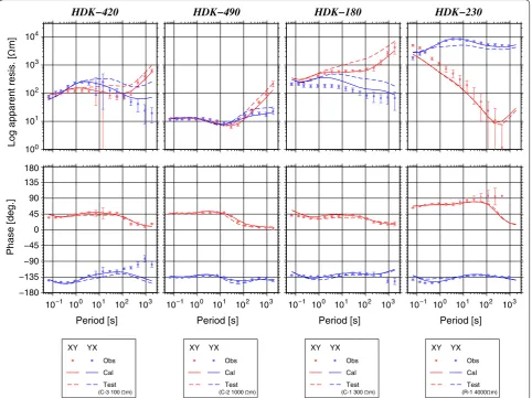
The calculated MT impedance tensors, which were converted to apparent resistivity and impedance phase

(Fig. 2, Additional file 1), showed considerable

varia-tion. Apparent resistivities were low (< 10 Ωm) beneath the Ishikari lowland and Tokachi Plain, but were high beneath the Hidaka metamorphic belt. The impedance phases showed out-of-quadrant phases in off-diagonal components at a few sites around the Shikotsu Caldera and Hidaka metamorphic belt (e.g., sites 420 and 230 in

Fig. 2). The out-of-quadrant phases possibly represent

the combined effect of two anisotropic layers, each with a

different anisotropic azimuth (e.g., Pek and Verner 1997;

Heise and Pous 2003), or channeling and bending of the

telluric current that requires resolution by 3-D

resistiv-ity modeling (e.g., Ichihara and Mogi 2009; Ichihara et al.

2013).

Phase tensor and induction vectors

We calculated the phase tensor (Caldwell et al. 2004)

and Parkinson’s induction vector (Parkinson 1962) to

(4)

that describes the phase relationship contained in the

MT impedance tensor (Caldwell et al. 2004). It

pre-serves the effect of regionally heterogeneous resistivity, whereas the MT impedance tensor is distorted by the galvanic effects produced by heterogeneity of near sur-face resistivity. The root of the determinant of the phase tensor is called Φ2. In the simple 1-D case, Φ2 > 45° and

Φ2 < 45° indicate decreasing and increasing resistivity,

respectively, with increasing depth.

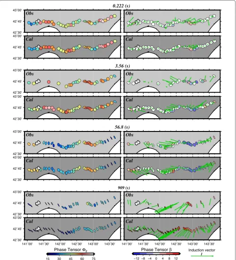
The phase tensor ellipses showed high Φ2

val-ues (> 60°) at 0.222 s under the Ishikari lowland and Tokachi Plain, but low values (< 30°) in these areas at

56.8 s (Fig. 3, Additional file 2). These observations

indicate that the shallow resistivity decreased with depth, whereas the deep resistivity increased with depth. In the area of the Hidaka metamorphic belt,

high Φ2 (> 50°) was estimated between 3.56 and 56.8 s,

implying decreasing resistivity with depth.

The azimuths of the principal axes of phase tensor ellipses, which indicate the azimuth of strike (or azimuth perpendicular to strike) of a resistivity structure in a 2-D model, were mostly aligned at 330° at 909 s. However, the azimuths of the principal axes varied considerably at shorter periods, indicating that the shallow electri-cal resistivity structure has strong three-dimensionality.

Absolute values of skew angle (β) were large (> 5°) at

peri-ods longer than 56.8 s at more than half of the MT sites, which is also an indicative of strong three-dimensionality.

Negative values of β at 56.8 s near the HCZ had become

positive at 909 s, which implies an asymmetric resistivity distribution.

The Parkinson’s induction vector is defined as the reverse vector of the real part of the geomagnetic trans-fer function, and it commonly points to a conductive

anomaly (Parkinson 1962). Parkinson’s induction vectors

between 3.56 and 56.8 s trend toward the Ishikari lowland

XY YX

Log apparent resis.

[

m]

HDK−420 HDK−490 HDK−180 HDK−230

XY YX

(5)

and the Tokachi Plain, which may indicate conductive areas there. They trend WSW with a maximum length of 0.7 at 909 s and can be attributed to current channeling

beneath the Ishikari Lowland because of the combination of conductors consisting of narrow conductive sediment

beneath the lowland and seawater (Yamaya et al. 2017).

1

15 30 45 60 75

Phase Tensor Φ2

909 (s) 56.8 (s) 0.222 (s)

Induction vector 141˚00' 141˚30' 142˚00' 142˚30' 143˚00' 143˚30'

42˚30' 42˚45' 43˚00'

141˚00' 141˚30' 142˚00' 142˚30' 143˚00' 143˚30' 42˚30'

42˚45' 43˚00' 42˚30' 42˚45' 43˚00' 42˚30' 42˚45' 43˚00'

−12 −8 −4 0 4 8 12 Phase Tensor β 42˚30'

42˚45' 43˚00' 42˚30' 42˚45' 43˚00' 42˚30' 42˚45' 43˚00' 42˚30' 42˚45' 43˚00'

3.56 (s) Obs

Cal

Obs

Cal

Obs

Cal

Obs

Cal

Obs

Cal

Obs

Cal

Obs

Cal

Obs

Cal

Fig. 3 Observed (OBS) and model-predicted (Cal) phase tensor ellipses and induction vectors. In the panels on the left, colored ellipses indicate

Φ₂ of the phase tensor. Observed data with large errors (Φ2 > 10°) are not shown. In the panels on the right, colored ellipses indicate β of the phase

(6)

Therefore, 3-D resistivity modeling that includes the presence of seawater is necessary to correctly estimate the subsurface resistivity distribution in the study area.

3‑D inversion

Although the MT stations were along a single line across the HCZ, we used 3-D rather than 2-D inversion for the following reasons. (1) The phase tensor ellipses and

induction vectors (Fig. 3) indicated strong

three-dimen-sionality of resistivity structures that 2-D modeling sometimes misinterprets. (2) 3-D inversions can provide more realistic images of resistivity structure beneath MT stations if those stations are along a single profile and the structure is strongly three-dimensional (e.g., Siripunvara-porn et al. 2005b).

We used 3-D inversion code WSINV3DMT

(Siripun-varaporn and Egbert 2009; Siripunvaraporn et al. 2005a).

The objective function consisting of model roughness term and data misfit term is minimized in the inversion. The former term allows to estimate broader resistivity anomaly compared to true anomaly. The inversion uses data-space formulation in the objective function and the Occam scheme to evaluate the balance of model rough-ness and data misfit. The settings and procedures we

used are provided in Additional file 3.

The sounding curves calculated from the inverted model agreed reasonably with the measured curves

(Fig. 2, Additional file 1) as did the measured phase

ten-sor ellipses and induction vectors (Fig. 3, Additional

file 2). However, high-amplitude diagonal components

of MT impedance and the geomagnetic transfer function at short periods were not well resolved at several sites

(Additional file 1), mainly because the horizontal mesh

size of the model (> 4 km) was too large to explain small-scale horizontal variations of resistivity.

Results and discussion

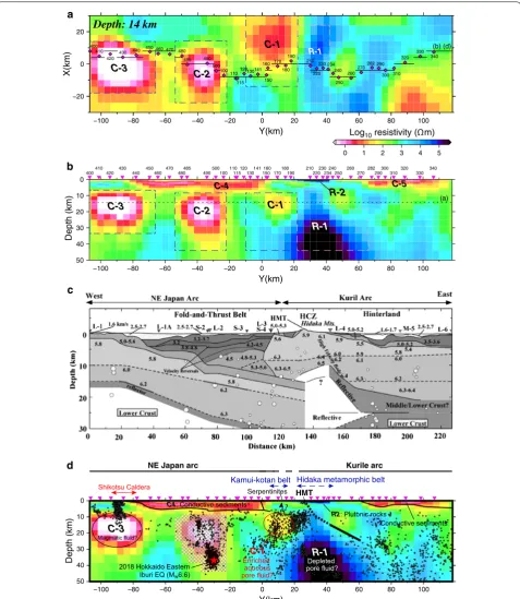
The inverted resistivity model (Fig. 4a, b) shows

signifi-cant resistivity variations: (1) three distinct low-resistivity anomalies (conductors) between 7 and 40 km depth on the NE Japan arc side of the HMT (C-1, C-2, and C-3), (2) two shallow conductive layers at 0–6 km depth beneath the Ishikari lowland (C-4) and Tokachi Plain (C-5), and (3) two resistive zones in the center of the HCZ (R-1 and R-2).

The anomalous conductor beneath the Shikotsu caldera (C-3) was verified by the sensitivity test, as

described in Additional file 4 (see also station HDK-420

in Figs. 2, 4a, b, and Table 1). It supports the

conduc-tive region previously identified by Yamaya et al. (2017)

(Additional file 5) because we used mostly different

MT dataset from they used. This conductive region

possibly represents a region of magmatic fluid beneath

the Shikotsu caldera as Yamaya et al. (2017) discussed.

However, we do not discuss the detailed resistivity

distribution in this area because Yamaya et al. (2017)

modeled more-detailed resistivity distribution (see

Additional file 4 for details).

Yamaya et al. (2017) detected a deep conductor

beneath the Ishikari-teichi-toen fault (C1 in Yamaya

et al. 2017) that our inverted resistivity model did not

reproduce (Additional file 5). We attribute its absence

in our model to the low sensitivity in the data due to following two effects. There is no MT site directly above the conductor. The electromagnetic field is atten-uated by surface conductor C-4 and thus is slightly pen-etrated beneath the C-4.

The low apparent resistivities at shorter periods

(Fig. 2, Additional file 1) and high Φ2 values of the

phase tensor (Fig. 3, Additional file 2) clearly suggest

the presence of the two shallow subsurface conductors C-4 and C-5, which are spatially consistent with areas

of low seismic velocity (Vp < 4.5 km/s) that were

inter-preted by Iwasaki et al. (2004) to represent Cretaceous

or younger sedimentary rocks (Fig. 4c, d). Previous MT

studies (Ichihara et al. 2008, 2016; Yamaya et al. 2017)

have also recognized thick near-surface conductors associated with the sedimentary rocks.

In the following sections, we discuss our interpreta-tions of the resistivity anomalies in the center of the HCZ (R-1, R-2, C1) and beneath the epicenter of the 2018 earthquake (C-2).

Interpretation of the conductor beneath Kamui‑kotan belt (C‑1)

The sensitivity tests (Additional file 4) demonstrated

that the observed data require the resistivity of C-1

to be lower than 300 Ωm (Table 1) and that the C-1

anomaly possibly extended to the north of the profile

(Fig. 4a). Ogawa et al. (1994) previously identified a

conductor around the center of the C-1 anomaly. The distribution of the C-1 anomaly is consistent with the surface distribution of serpentinite mélange in the Kamui-kotan belt. In addition, seismic tomographic modeling has shown an area of high attenuation of seis-mic energy beneath the Kamui-kotan belt (Kita et al.

2014). Such attenuation is a characteristic of rocks

con-taining aqueous pore fluids. Thus, we interpret the C-1 anomaly to represent a zone enriched in aqueous pore fluid. Because geological studies have suggested that the root of serpentinitic material in the middle crust is

in the region of C-1 (Katoh 2018; Ueda 2006), the C-1

(7)

0

410 430 450 470 485 500

100 115 130 150 170 190 220 234 250 270 290 310 330

400 420 440 460 480 490

X(km)

430 440 450 460 470 480 485 490

R2: Plutonic rocks

C4: Conductive sediments

Conductive sediments

Kamui-kotan belt Hidaka metamorphic belt

NE Japan arc Kurile arc

a

b

c

d

Fig. 4 Interpreted 3-D resistivity model. a Horizontal section of the inverted resistivity model at 14 km depth. Dashed lines show areas of sensitivity

tests (where resistivity values were replaced). b Vertical cross-section beneath an east–west line around MT stations assembled from short east–

west profiles shown as solid lines in a. Dotted line marks the horizontal position of a. c Interpreted seismic velocity section (from Iwasaki et al.

2004). The location of the seismic survey line corresponds closely to that of the MT survey line of this study. d Interpretations superimposed on

the vertical cross-section of b. The red star denotes the hypocenter of the 2018 Hokkaido Eastern Iburi earthquake (Mw 6.6). The small circles

denote hypocenters of earthquakes between 2001 and 2019. The red circles indicate hypocenters occurred after the 2018 Hokkaido Eastern Iburi

(8)

Resistive bodies beneath the Hidaka metamorphic zone (R‑1 and R‑2)

High apparent resistivities between sites 210 and 234

(see site 230 in Fig. 2) correspond to the surface

resis-tive zone of the Hidaka metamorphic belt (R-2), which contains granulite and plutonic rocks. The electri-cal resistivity of dry granulite from this area is high

(2000 Ωm at 570 K; Fuji-ta et al. 2004). Moreover, dry

plutonic rocks under surface conditions generally show high resistivity. Thus, the R-2 anomaly can be explained by the presence of granulite and plutonic rocks. The distribution of the eastern part of the R-2 anomaly is consistent with the distribution of plutonic rocks identified from gravity survey data (Kamiyama et al.

2005). Alternatively, the area of relatively low resistivity

beneath the R-2 anomaly can be interpreted to repre-sent metasedimentary rocks, as discussed by

Kamiy-ama et al. (2005).

Sensitivity modeling showed that the R-1 high-resis-tivity anomaly (> 4000 Ωm) is at depths around the

middle crust (Additional file 4). Based on the surface

trace of the HMT and a dipping seismic reflector

previ-ously observed in the middle crust (Iwasaki et al. 2004),

the R-1 anomaly is within the footwall of the HMT

(Fig. 4d). In contrast, Ichihara et al. (2016) identified

a conductive zone in the footwall of the HMT in the southern part of the HCZ and interpreted it to repre-sent dehydration fluid flow from the Pacific plate

(Addi-tional file 5). Such variations of resistivity along the

footwall of the HMT possibly reflect a dependence of the supply of dehydration fluid on the depth of the plate boundary. However, resistivity distribution between the C-1 and R-1 anomalies is not constrained because of the sparse MT coverage between sites 190 and 210

(Fig. 4). More-detailed observations with a gridded

array of MT sites are essential to obtain a detailed 3-D resistivity model for this anomaly.

Conductive anomaly (C‑2) near the hypocenter of 2018 Hokkaido Eastern Iburi earthquake

We applied a sensitivity test (as for the C-1 anomaly) to

the C-2 anomaly (see Fig. 4, Table 1, Additional file 4),

which lies above the hypocenter of the 2018 Hokkaido

Eastern Iburi earthquake. Yamaya et al. (2017) also

showed a weak conductive anomaly in the area of our C-2

anomaly (Additional file 5). Although the sensitivity test

degraded the fit of the sounding curves to the observed

data (see station 490 in Fig. 2), the RMS misfit was

insuf-ficiently different from that of the final model to satisfy

the F-test (Table 1, Additional file 4). Therefore, the

observed data we used cannot resolve conductive area C-2. We suggest that attenuation of the electromagnetic field by surface conductor C-4 above the C-2 anomaly decreased the strength of the MT response of the under-lying rocks.

To further clarify the resistivity distribution in the area of the C-2 anomaly, we need to increase data quality and quantity to overcome the effect of attenuation of the magnetic field by shallow conductors. The C-2 anomaly has sensitivity to the MT response around the site 490 and will be demonstrated by additional MT

measure-ments (Additional file 4). If the modeled C-2 conductor is

indeed genuine, it may represent a region rich in pore

flu-ids that control fault rupture (e.g., Scholz 2002). It would

therefore be a key to understand the anomalous faulting in the HCZ. Therefore, denser MT survey data coverage is required around the epicentral area of the 2018 Hok-kaido Eastern Iburi earthquake.

Conclusions

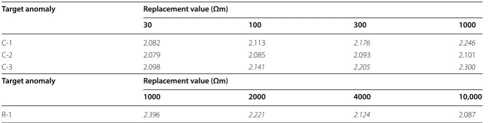
We used 3-D inversion to reanalyze MT imped-ances and geomagnetic transfer functions beneath an east–west transect that crosses the HCZ and the focal zone of the 2018 Hokkaido Eastern Iburi earthquake. The resultant electrical resistivity model showed a Table 1 RMS misfits obtained in sensitivity tests of the inverted electrical resistivity model

For target anomalies named with a leading “R” (or “C”), only the blocks with higher (or lower) resistivities than that shown in the “Replaced value” column were replaced. Italic RMS misfits indicate a model significantly different from the inverted model. The RMS misfit for the final inverted model was 2.082, and all models have 7296 degrees of freedom

Target anomaly Replacement value (Ωm)

30 100 300 1000

C-1 2.082 2.113 2.176 2.246

C-2 2.079 2.085 2.093 2.101

C-3 2.098 2.141 2.205 2.300

Target anomaly Replacement value (Ωm)

1000 2000 4000 10,000

(9)

near-surface high-resistivity zone (R-2) beneath the Hidaka metamorphic belt that we interpreted to repre-sent elevated mid-crustal plutonic rocks and granulite. Beneath resistive zone R-2, we identified a deep resis-tive zone R-1 on the footwall of the HMT, although

Ichihara et al. (2016) identified conductive zones on

this side of the fault in the southern part of the HCZ. The variations of resistivity we modeled possibly reflect variations of the amount of aqueous pore fluid supplied from the subducting Pacific plate. West of resistive zone R-1, we identified conductive zone C-1 beneath

the high P–T metamorphic Kamui-kotan belt. Because

the C-1 conductive zone is spatially related to the ser-pentinite mélange of the Kamui-kotan belt, it likely represents a zone of enriched pore fluid related to the formation of the serpentinite. The resistivity model also showed a conductive anomaly (C-2) above the hypo-center of the 2018 Hokkaido Eastern Iburi earthquake; however, this anomaly was not resolved by our mod-eling owing to the sparse coverage and poor quality of the MT data we used. Additional dense MT surveys of high quality in the area around the epicenter of the 2018 earthquake will clarify the existence and distribu-tion of that conductor and make an important contri-bution to our understanding of fault rupture processes in the deep crust in the HCZ.

Supplementary information

Supplementary information accompanies this paper at https ://doi. org/10.1186/s4062 3-019-1078-7.

Additional file 1. Sounding curves. Apparent resistivity and phase of MT impedance are shown in upper and middle boxes, respectively. Tipper amplitudes are shown in lower boxes. Symbols labeled with “Obs” and “Cal” indicate observed and model-predicted MT responses, respectively.

Additional file 2. Pseudosections of observed (OBS) and model-predicted (Cal) Φ2 (upper two panels) and β (lower two panels) of phase tensor ellip-ses. Observed data with large errors (Φ2 > 10°, β > 5°) are not shown.

Additional file 3. Settings and procedures for 3-D inversion.

Additional file 4. Verification of resistivity anomalies by sensitivity tests.

Additional file 5. Comparison of the inverted 3-D resistivity model of this study with these of Yamaya et al. (2017) and Ichihara et al. (2016).

Abbreviations

MT: magnetotelluric; HCZ: Hidaka collision zone; HMT: Hidaka main thrust.

Acknowledgements

We thank the members of the Hidaka 2000 MT observation group and Dr. Hiroyuki Kamiyama (Ueyama-shisui Co. Ltd.) for making the MT data available for this study. Continuous geomagnetic records by the Esashi geomagnetic observatory, Geospatial Information Authority of Japan, were used for remote references. Comments from Prof. H. Takahashi and Prof. Takeshi Hashimoto of Hokkaido University and two anonymous reviewers improved the manuscript. We used computer systems at the Earthquake and Volcano Information Center, Earthquake Research Institute, The University of Tokyo, for 3-D inver-sion and sensitivity tests. Generic Mapping Tools software (Wessel and Smith

1998) was used to draw the figures.

Authors’ contributions

All authors contributed to the analyses of data and interpretation of the resistivity modeling and approved the final manuscript. All authors read and approved the final manuscript.

Funding

This research was supported in part by a grant from the Japanese Ministry of Education, Culture, Sports, Science and Technology, KAKENHI Grant no. 18K19952.

Availability of data and materials

The corresponding author can be contacted to access the digital data under-pinning the 3-D resistivity model.

Ethics approval and consent to participate

Not applicable.

Consent for publication

Not applicable.

Competing interests

The authors declare that they have no competing interests.

Author details

1_{Earthquake and Volcano Research Center, Graduate School of Environmental} Studies, Nagoya University, Furo-cho, Chikusa-ku, Nagoya 464-8601, Japan. 2_{Division of Sustainable Resources Engineering, Graduate School of} Engineer-ing, Hokkaido University, N13W8, Sapporo 060-8628, Japan. 3_{Volcanic Fluid} Research Center, School of Science, Tokyo Institute of Technology, Tokyo, Japan. 4_{Nuclear Regulation Department, Secretariat of Nuclear Regulation} Authority, 1-9-9, Roppongi, Minato-ku, Tokyo 106-8450, Japan. 5_Renewable Energy Research Center, Fukushima Renewable Energy Institute, AIST, 2-2-9 Machiikedai, Koriyama, Fukushima 963-0298, Japan.

Received: 5 March 2019 Accepted: 26 August 2019

References

Amante C, Eakins BW (2009) ETOPO1 1 Arc-minute global relief model: procedures, data sources and analysis. NOAA Technical Memorandum NESDIS NGDC-24. National Geophysical Data Center, NOAA. https ://doi. org/10.7289/v5c82 76m

Caldwell TG, Bibby HM, Brown C (2004) The magnetotelluric phase tensor. Geophys J Int 158:457–469

Fuji-ta K, Katsura T, Tainosho Y (2004) Electrical conductivity measurement of granulite under mid- to lower crustal pressure–temperature conditions. Geophys J Int 157:79–86

Gamble TD, Clarke J, Goubau WM (1979) Magnetotellurics with a remote magnetic reference. Geophysics 44:53–68

Heise W, Pous J (2003) Anomalous phases exceeding 90° in magnetotel-lurics: anisotropic model studies and a field example. Geophys J Int 155:308–318

Ichihara H, Mogi T (2009) A realistic 3-D resistivity model explaining anomalous large magnetotelluric phases: the L-shaped conductor model. Geophys J Int 179:14–17. https ://doi.org/10.1111/j.1365-246X.2009.04310 .x

Ichihara H, Honda R, Mogi T, Hase H, Kamiyama H, Yamaya Y, Ogawa Y (2008) Resistivity structure around the focal area of the 2004 Rumoi-Nanbu earthquake (M 6.1), northern Hokkaido, Japan. Earth Planets Space 60:883–888. https ://doi.org/10.1186/Bf033 52841

Ichihara H, Mogi T, Yamaya Y (2013) Three-dimensional resistivity modelling of a seismogenic area in an oblique subduction zone in the western Kurile arc: constraints from anomalous magnetotelluric phases. Tectonophysics 603:114–122. https ://doi.org/10.1016/j.tecto .2013.05.020

(10)

Iwasaki T, Adachi K, Moriya T, Miyamachi H, Matsushima T, Miyashita K, Takeda T, Taira T, Yamada T, Ohtake K (2004) Upper and middle crustal deforma-tion of an arc–arc collision across Hokkaido, Japan, inferred from seismic refraction/wide-angle reflection experiments. Tectonophysics 388:59–73 Japan Meteorological Agency (2019) The seismological Bulletin of Japan.

http://www.data.jma.go.jp/svd/eqev/data/bulle tin/index _e.html. Accessed 8 June 2019

Kamiyama H, Yamamoto A, Hasegawa T, Kajiwara T, Mogi T (2005) Gravity and density variations of the tilted Tottabetsu plutonic complex, Hok-kaido, northern Japan: implications for subsurface intrusive structure and pluton development. Earth Planets Space 57:E21–E24. https ://doi. org/10.1186/BF033 51894

Kato N, Sato H, Orito M, Hirakawa K, Ikeda Y, Ito T (2004) Has the plate bound-ary shifted from central Hokkaido to the eastern part of the Sea of Japan? Tectonophysics 388:75–84

Katoh T (2018) A geological east-west cross section through the Iwanai-dake peridotite mass in Hidaka town based on the tectogenesis of ultramaic masses, Hokkaido. Bull Hidaka Mt Mus Hidaka Mt Res 1:21–30 Kimura G (1986) Oblique subduction and collision—Fore-arc tectonics

of the Kuril Arc. Geology 14:404–407. https ://doi.org/10.1130/0091-7613(1986)14%3c404 :Osacf t%3e2.0.Co;2

Kita S, Hasegawa A, Nakajima J, Okada T, Matsuzawa T, Katsumata K (2012) High-resolution seismic velocity structure beneath the. J Geophys Res-Solid Earth. https ://doi.org/10.1029/2012j b0093 56

Kita S, Nakajima J, Hasegawa A, Okada T, Katsumata K, Asano Y, Kimura T (2014) Detailed seismic attenuation structure beneath Hokkaido, northeastern Japan: Arc-arc collision process, arc magmatism, and seismotectonics. J Geophys Res-Solid Earth 119:6486–6511. https ://doi.org/10.1002/2014j b0110 99

Mogi T, Hidaka 2000 MT Group (2002) Broadband MT surveys in Hidaka area. Monthly Chikyu 24:485–487 (in Japanese)

Ogawa Y, Nishida Y, Makino M (1994) A collision boundary imaged by mag-netotellurics, Hidaka Mountains, Central Hokkaido, Japan. J Geophys Res-Solid Earth 99:22373–22388

Parkinson WD (1962) The influence of continents and oceans on geomagnetic variations. Geophys J R Astron Soc 6:441–449

Pek J, Verner T (1997) Finite-difference modelling of magnetotelluric fields in two-dimensional anisotropic media. Geophys J Int 128:505–521 Scholz CH (2002) The mechanics of earthquakes and faulting, 2nd edn.

Cam-bridge University Press, CamCam-bridge

Sibson RH (1990) Rupture nucleation on unfavorably oriented faults. Bull Seismol Soc Am 80:1580–1604

Siripunvaraporn W, Egbert G (2009) WSINV3DMT: vertical magnetic field transfer function inversion and parallel implementation. Phys Earth Planet Interiors 173:317–329. https ://doi.org/10.1016/J.Pepi.2009.01.013

Siripunvaraporn W, Egbert G, Lenbury Y, Uyeshima M (2005a) Three-dimen-sional magnetotelluric inversion: data-space method. Phys Earth Planet Interiors 150:3–14

Siripunvaraporn W, Egbert G, Uyeshima M (2005b) Interpretation of two-dimensional magnetotelluric profile data with three-two-dimensional inver-sion: synthetic examples. Geophys J Int 160:804–814

Ueda H (2006) Geologic structure of Cretaceous accretionary complexes in the frontal Hidaka collision zone, Hokkaido, Japan. J Geol Soc Jpn 112:699–717

Wessel P, Smith WHF (1998) New, improved version of Generic Mapping Tools released. EOS Trans Am Geophys Union 79(47):579

Yamaya Y, Mogi T, Honda R, Hase H, Hashimoto T, Uyeshima M (2017) Three-dimensional resistivity structure in Ishikari Lowland, Hokkaido, northeast-ern Japan—implications to strain concentration mechanism. Geochem Geophys Geosyst 18:735–754. https ://doi.org/10.1002/2016g c0067 71

Publisher’s Note