FULL PAPER
Development of a modified
envelope correlation method based
on maximum-likelihood method
and application to detecting and locating deep
tectonic tremors in western Japan
Naoto Mizuno
*and Satoshi Ide
Abstract
We develop a modified envelope correlation method for locating deep tectonic tremors and apply it to construct a tremor catalog for western Japan. We redefine the envelope cross-correlation method as a maximum-likelihood method by using the cross-correlation functions as objective functions and then weighting components of the data by the inverse of the error variances. This method is also capable of detecting multiple sources that occur almost simultaneously because they appear as local maxima in our analysis. We employ a nonlinear function, the average of the weighted cross-correlation functions (ACC), to locate the deep tectonic tremor hypocenters. Our optimization method is performed in two steps. We first fix the source depth and use a grid search to find the local ACC maxima, which are the potential event locations. We then use each potential event location as an initial value and apply the gradient method to determine its hypocentral location. Several source locations are sometimes determined in a 5-min time window. We also perform a numerical test using synthetic waveforms to validate our tremor hypocenter estimations. We apply our proposed method to continuous seismograms in western Japan for 12.5-year period, with our new approach detecting 35% more tremors than the envelope correlation method with the outlier control owing to the detection of multiple tremors in a single time window and to the improved tremor hypocenter accuracy yielded by the appropriate weighting scheme. We estimate the spatial resolution, which is defined as the epicentral distance between sources that can be distinguished by the location method, to be ~ 100 km.
Keywords: Deep tectonic tremor, Hypocenter determination, Envelope correlation method, Maximum-likelihood method, Western Japan
© The Author(s) 2019. This article is distributed under the terms of the Creative Commons Attribution 4.0 International License (http://creat iveco mmons .org/licen ses/by/4.0/), which permits unrestricted use, distribution, and reproduction in any medium, provided you give appropriate credit to the original author(s) and the source, provide a link to the Creative Commons license, and indicate if changes were made.
Introduction
Since the first discovery of deep tectonic tremors in the Nankai Subduction Zone (Obara 2002), tremors and similar slow slip phenomena have been observed in many subduction zones, such as Cascadia (Rogers and Dragert
2003), Mexico (Payero et al. 2008), Alaska (Peterson and Christensen 2009), and Costa Rica (Brown et al. 2009). Shelly et al. (2007) showed that tremors consist of many
low-frequency earthquakes (LFEs), which are tiny shear slips on the deep extension of the plate boundary where megathrust earthquakes occur repeatedly. Tremors are considered the short-period component of broad-band slow earthquakes, spanning from LFEs, which are observed above 1 Hz, to slow slip events, with durations of several days to several months, as recently discovered in the shallower section of the plate interface in the Nan-kai Subduction Zone (Ide et al. 2007; Kaneko et al. 2018). Tremors may therefore be useful for accurately monitor-ing the slow deformation behind them. The proximity of the source regions of slow and megathrust earthquakes
Open Access
*Correspondence: [email protected]
suggests some interaction between these slow and fast processes (e.g., Obara and Kato 2016). The accurate and complete monitoring of tremors is therefore an essen-tial component in investigating the potenessen-tial interactions between these slow and ordinary earthquake phenomena.
Ordinary location methods using phase arrivals and S–P lag times are not applicable for locating tremors because tectonic tremor waveforms lack clear P- and S-wave phases. Various tremor location methods have been developed to address this issue. The method used in the first discovery of tremors in the subduction zone of western Japan was the envelope correlation method (Obara 2002). The envelope correlation method analyzes the similarity of the envelope waveforms between seis-mic stations and locates a tremor source to explain the observed travel time differences of the tremor signals measured by maximizing the cross-correlations of enve-lope waveforms, with the travel times being calculated using ray theory. A number of improvements to the enve-lope correlation method have since been proposed. The method of Wech and Creager (2007, 2008) determined tremor locations by directly maximizing the cross-cor-relations of the envelope waveforms. Maeda and Obara (2009) incorporated signal amplitude information into the envelope correlation method. Ide (2010) determined an event with a finite duration in the time window to demonstrate the effectiveness of outlier-control schemes.
The matched-filter method (e.g., Gibbons and Ring-dal 2006) is another popular approach for tremor sig-nal detection. Shelly et al. (2007) detected a number of tremors using the highest quality LFEs as template events in the matched-filter method and showed that tremors occur as a swarm of LFEs. Brown et al. (2008) developed an autocorrelation method for tremor detection. Bos-tock et al. (2012) extended these methods by preparing template waveforms consisting of stacking many LFEs detected by short-period autocorrelations and used them as template events. Although these methods generally provide more accurate and complete tremor detection and location, they generally have tremendous computa-tional requirements and are not always suitable for large datasets that consist of many stations over a large area and long observation period.
Several other techniques have also been implemented for tremor detection and location. The source scanning algorithm of Kao and Shan (2004) estimates the tremor location and origin time that maximizes the brightness, which is the sum of the absolute amplitudes shifted by the theoretical travel times. La Rocca et al. (2010) showed that the cross-correlation between the vertical and hori-zontal seismogram components recorded by dense seis-mic arrays could be utilized to determine the S–P times of the tremor signals, with this information improving
the accuracy of the tremor source location. Rubin and Armbruster (2013) showed that the tremor waveforms at two stations separated by 10–20 km were sometimes quite similar and could be used to measure the relative arrival time via cross-correlation. Their algorithm, the cross-station method, utilizes this similarity and locates tremors accurately using seismograms from only three stations.
The applicability of tremor location methods depends on the properties of seismic data, such as the extent of the target region, the observation period, and the num-ber of stations. Here, we develop a method suitable for either a large data volume from many stations covering a long duration or daily monitoring. We review the meth-odology of current envelope correlation methods (Obara
2002; Wech and Creager 2008) from a statistical view-point and develop a location algorithm that is sufficiently fast, accurate, and applicable to a huge data volume. We apply this method to the seismogram records from 313 seismic stations in western Japan to construct a tremor catalog in the Nankai Subduction Zone for the period April 2004 to September 2016.
Method
Maximum‑likelihood‑based location method
Our proposed method is essentially equivalent to that proposed by Wech and Creager (2007, 2008), but with the key modification of employing slightly different mathematical expressions that are introduced from a the-oretical perspective based on the maximum-likelihood method.
Suppose that we analyze a set of continuous envelope waveforms from ground velocity seismograms sampled at time interval ΔT and search for tremors within a fixed time window with a width Tw=NtΔT, where Nt is the
number of time samples. We define the normalized enve-lope waveform wi(t) in this time window as
where the subscript i indicates the i-th component, wi′(t)
is the original envelope waveform, w′i is its temporal
mean, and tk is the k-th time step in the window.
We assume that the envelope shape is common for all components at all stations. This means that each observa-tion (normalized envelope waveform) wi(t) is represented
by the summation of a common template waveform w(t) that is time-shifted because of seismic wave propagation from the source and Gaussian error ei(t) with a
where Δti(x) is the travel time from a potential source
position x to the station recording the i-th component. The likelihood of obtaining the observed envelopes L(w,
x) for a given combination of w(t) and x is written as
where N is the number of envelope components at all available stations. The log-likelihood is
For a fixed source location, Eq. (4) shows that we can determine the w(tk) that maximizes the log-likelihood at
each discrete time tk independently, which is equivalent
to minimizing
for w(tk). We can determine the maximum-likelihood
estimate wMLE(t
k, x) by taking the derivative of Eq. (5)
with respect to w(tk), which is considered the best
tem-plate waveform and is written as
The maximum log-likelihood is then rewritten as
Assuming that the data possess a periodicity, where
wi(t) =wi(t +Tw), the summation of the first term for k is
independent of x. Therefore, we can essentially maximize the likelihood with x by simply maximizing the second term, which is rewritten as
(2)
We then substitute Eq. (6) into the above formula to obtain
By combining the x-dependent terms, we find the max-imum of Eq. (9) is obtained by maximizing
This can be rewritten as
which is a summation of the cross-correlations weighted by the inverse of the error variances. The best tremor location in the analyzed time window is therefore deter-mined by calculating the Δti(x) value (and therefore x)
that maximizes Eq. (11). This function is identical to the maximized function in Wech and Creager (2007, 2008), except the weighting factors for cross-correlations. Note that the variance σi2 is fixed to estimate the likelihood
function because it is determined from other informa-tion, which is discussed below.
The practical application of our proposed method requires that we use only those pairs of envelope wave-forms whose cross-correlation maximum is larger than a threshold Clim. This criterion removes station pairs that
may violate the assumption in Eq. (2) that the normalized envelope waveforms are the sum of the template wave-form and small random errors, and also accelerates the computation. The resultant objective function to maxi-mize in the numerical calculation is
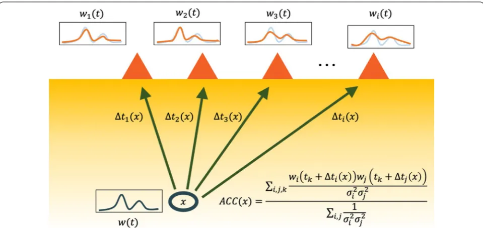
We introduce the average of the weighted cross-corre-lations (ACC) as the final function to maximize for x as
where the criterion for Clim is omitted. This approach also
allows us to compare the objective functions for different weight settings. Equation (13) is equivalent to Eq. (12) when the variances are fixed. Figure 1 shows a schematic diagram of our proposed location method.
Our ACC evaluation requires numerous evaluations of the correlation functions. We calculate the cross-correlations for each pair with travel time differences in the frequency domain via the fast Fourier transform method, as time differences are multiples of the sampling interval, and then store the cross-correlations in a table to reduce the computational requirements and costs of the method. We optimize our proposed method by cal-culating the cross-correlations as spline interpolations of values in our calculated table. By referring to this table, we can reduce the number of the evaluations of the cross-correlation functions between station pairs as much as the original envelope correlation method.
ACC optimization
We search for the maximum ACC using a combination of a grid search and a gradient method. The grid search, assuming a fixed tremor depth, picks several local ACC maxima as potential tremor epicenter locations. The vari-ances of the normalized envelope waveform error σi2 are
assumed to be proportional to the square of the hypo-central distance during this first step of the optimization. Note that we consider local maxima instead of the global maximum. This is because multiple tremors may occur at different locations in the same time window, such that the local maxima may reflect the occurrence of multiple tremors in a single time window.
We then maximize ACC using a gradient method, the conservative convex separable approximation (CCSA) algorithm (Svanberg 2002), with each potential tremor epicenter being used as an initial value, to determine the best hypocentral location of each tremor. When the hypocentral solutions from some potential locations are very close to each other, we unite these solutions.
We simply assume that the variances in the normalized envelope waveform errors are proportional to the square of the hypocentral distance in the grid search stage and locate potential tremor source epicenters. We then recal-culate the weights assuming that the variances are pro-portional to the squared difference between wi and wMLE,
such that
(14) σi2∝
Nt
k=1
wi(tk+�ti(x))−wMLE(tk,x) 2
A given seismic dataset may include very unusual observations that are unexpected in Gaussian statistics. We therefore employ two criteria to remove any outliers after the first tremor source estimation and repeat the procedure with the refined dataset until no outliers are identified.
The first criterion is based on the envelope cross-correlation, which requires each waveform in a pair of normalized envelope waveforms to meet a threshold cross-correlation Clim for consideration in the analysis.
We originally apply the criterion about the cross-corre-lation to select the pairs in Eq. (12), which means that the maximum of the cross-correlation function is always larger than Clim. However, the cross-correlation value at
a given time lag, which is calculated based on the poten-tial tremor source location, is equal to or lower than the maximum and may be smaller than Clim.
The second criterion is based on the similarity between the envelope and the template waveform. We reject an envelope when the cross-correlation of the envelope and the template is below the threshold Climt . This criterion is
introduced to eliminate signals that occurred at differ-ent locations. In this case, the cross-correlation of the pair may possibly be large, such that the pair meets the first criterion, whereas the second criterion is designed to reject these different seismic signals. We repeat the pro-cedure, where we estimate σi, remove the outliers, and
maximize ACC via the CCSA algorithm until no outliers are identified, to determine the best tremor hypocenter
xbest.
We estimate the tremor source location error using a bootstrap method. We randomly resample the same number of correlated component pairs allowing duplica-tion and locate the tremor source. We repeatedly exam-ine the above process Nb times and determine the error
as the standard deviation of these calculated source locations.
Source parameter estimation
We determine the hypocentral time, duration, and energy magnitude of each detected tremor as
(15)
Ri is the hypocentral distance to the station recording the
i-th component; and ρ and β are the density and S-wave velocity at the station, which are assumed as 3,000 kg/ m3 and 2.844 km/s, respectively. The hypocentral time
is defined as the time when the maximum E˙s(t) occurs.
The tremor duration is also estimated as the period when
˙
Es(t) exceeds a quarter of its maximum. The energy
mag-nitude Me is defined as (Choy and Boatwright 1995)
with the integration taken over the tremor duration.
Application to observed data Data and preprocessing
The seismic data consist of continuous velocity wave-forms recorded at 313 Hi-net stations in western Japan maintained by the National Research Institute for Earth Science and Disaster Resilience. We only use the two horizontal components in our analysis because the tremor signals are dominated by S waves, and we want to suppress any unwanted P-wave signature, which is com-monly visible in the vertical component at some stations. The seismic data cover the period April 2004 to Septem-ber 2016, with the original records consisting of ground velocities sampled at 100 samples per second. The seis-mic data undergo a preprocessing procedure, which includes bandpass filtering at 2–8 Hz, squaring, low-pass filtering below 0.2 Hz, and resampling at 1 Hz, with the square root of the data considered as the envelope.
Parameter settings
The time window for the analysis Tw is fixed at 300 s. We
analyze the continuous data using half-overlapping suc-cessive time windows. Cross-correlation functions are calculated for all component pairs whose inter-station distances are less than 100 km. The detection method is applied to a given time window when the number of correlations that exceed the threshold of cross-correlation, Clim, is larger than 15. The travel time is
cal-culated using ray theory and the JMA2001 1-D velocity model (Ueno et al. 2002) as the assumed S-wave velocity structure.
The following optimization parameters are assumed. The spatial interval for the grid search is 0.2°. The search area is limited to the region covered by the observation
(16)
Me=
log ˙
Es(t)dt−4.4
network, with every grid point within 100 km of the nearest station. The source depth is assumed to be 30 km in the grid search, which is a typical tremor depth in this region. We pick a grid point if it is the local maximum around 1° × 1° section, which we use as the initial loca-tions in the gradient method. We merge the soluloca-tions when the distance between two solutions from the gra-dient method is less than 0.2°. The thresholds for outlier rejection, Clim and Climt , are set to 0.6 and 0.4, respectively.
We control the quality of the solution in several ways. The error is estimated via the bootstrap method, with
Nb = 100. We remove any tremors where the error is
greater than 2 km. We also apply a clustering technique to remove any spatiotemporally isolated solutions. We reject an event if it has no neighboring event within
± 0.2° latitude and longitude and ± 1 day. This method also detects ordinary earthquakes and does not distin-guish them from tremors. We therefore select events with durations previously defined of longer than 10 s as tremors because ordinary earthquake signals are shorter than tremor signals.
Tremor detection examples
We encounter numerous scenarios for identifying deep seismic tremors across the study region, including a single tremor (Fig. 2), multiple tremors (Figs. 3, 4), and closely spaced tremors (Fig. 5). Here, we provide specific examples of the common tremor scenarios during the analysis and describe how we distinguish the detected tremors in each scenario.
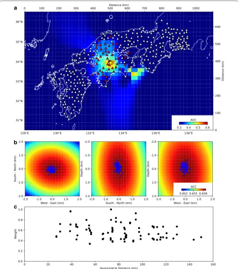
Figure 2a shows an example of the estimated tremor location, together with the spatial ACC distribution. The first grid search successfully selects the potential epi-central location that yields the maximum ACC, which represents a tremor source location, as the peak ACC dis-tribution is near the final location. The ACC disdis-tribution around the source is monophasic and suitable for further analysis via the gradient method (Fig. 2b). The bootstrap method results (blue dots) are concentrated in the high cross-correlation area. Figure 2c shows the relationship between the station distance and final weights, which have been adjusted during the iterative refinement. The weighting tends to decrease as the distance increases, which is consistent with the increased effect of seismic wave attenuation at greater distances. We successfully
reduce the effects of distant stations using this weighting scheme, where the signal qualities are generally poor.
We can potentially locate more than one event in a single time window by analyzing the local maxima. The ACC distribution in some cases shows two or more local maxima, suggesting that several events occurred. Fig-ure 3a shows an example analysis for a time window that captures two events. The tremor locations are denoted by the two stars, highlighting that they are well detected by these local ACC maxima. Figure 3b, c shows the time-shifted envelope waveforms calculated from each detected tremor location. The envelope waveform peaks are aligned systematically when the stations are near the epicenter. The waveform components of the distant sta-tions are automatically removed for each local maximum as a result of the outlier control scheme. In Fig. 3c, we can see the undetected peek around 180 s. Because we do not consider the temporal separation in a single time window, we only detect the largest signal. Therefore, the resolution of the temporal separation is limited by the length of the time window, 300 s.
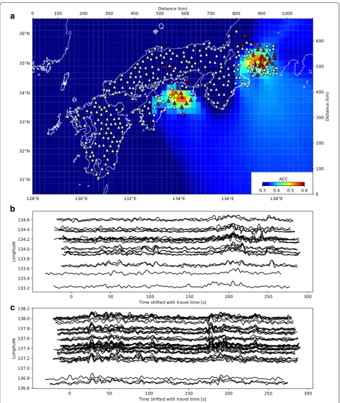
Figure 4 shows another multi-tremor example, with the location method detecting three events in a single time window. We note that there was persistent tremor activ-ity near each detected location for several hours prior to this time window.
The event separation may not be as large as that shown in previous examples. Figure 5 shows an example of a dif-ficult source location scenario, where two nearby events occurred. The signals from both events appear in the envelope waveforms recorded at some stations. Never-theless, our proposed method is able to successfully sepa-rate these two events.
The number and distribution of detected tremors
a
b
c
a
b
c
as 65,323 new events. Many of the missed events that were detected by the method of Ide (2010) are rejected on account of the short estimated tremor durations.
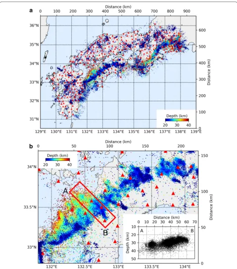
Figure 6 shows the detected tremor hypocenters via our proposed location method. Tremors are located in the vicinity of the plate boundary, which is consistent with the previous study. Our method also detects events outside of the tremor concentrated band. These include volcanic tremors and events occurring in Tottori (Ohmi and Obara 2002), Osaka Bay (Kamaya and Katsumata
2004; Aso et al. 2011), Kyushu (Yabe and Ide 2013), and Okayama (Ide and Tanaka 2014).
Discussion
Resolution of the location method
A unique feature of our proposed method is the detec-tion of multiple tremor events in a single time window.
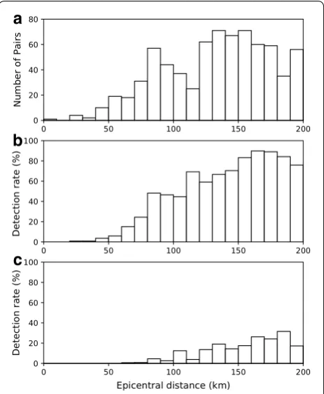
However, a pair of tremor events may be difficult to rec-ognize if they occur too close to each other. Therefore, we should determine the minimum separation required to detect multiple independent events. Figure 7a shows the number of detected tremor pairs by epicentral distance. There is a marked decrease in the simultaneous detection of event pairs in a single time window when the epicen-tral distance is less than 100 km, suggesting that the reso-lution of our method is ~ 100 km.
distribution with P(x) =e−x. The duration and magnitude
of Td are adjusted to the catalog value. The tremor focal
mechanism is assumed to be that of the moment tensor (strike = 228°, dip = 20°, and rake = 93°) determined for stacked broadband records by Ide and Yabe (2014). We then apply the location method to these synthetic wave-forms. Figure 7b shows the effectiveness of the location method in detecting two sources based on their epi-central distance, confirming that an epiepi-central distance of ~ 100 km is required between two tremor sources to locate them separately.
Weighting scheme
Our weighting scheme provides a major improvement. The implementation of our weighting scheme increases
the number of detected tremors from 55,327 to 132,704. The weighting scheme also reduces the tremor loca-tion errors and improves the resoluloca-tion of simultaneous tremor events. These improvements gained from imple-menting the weighting scheme can be seen by comparing the results with (Fig. 7b) and without (Fig. 7c) weighting factors. Simultaneous tremor events cannot be detected when weighting factors are not applied, highlighting the effectiveness of the weighting scheme in recognizing tremors that are spatiotemporally close to each other.
The effect of outlier controls
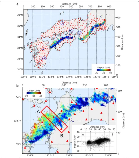
Outlier controls affect the number of detected tremor sources and their associated errors. Figure 8 shows the result when we ignore the second criterion. Although
this approach increases the number of detected events to 236,451, the resultant tremor sources are scattered over a broader region, suggesting numerous false detec-tions and larger location errors. Most of these events are falsely located or falsely assigned longer duration because of outlier data.
Conclusions
Here, we developed a new location method for deep tec-tonic tremors that is based on the envelope correlation method. We reviewed the relationship between the enve-lope correlation and maximum-likelihood methods and determined that envelope correlation weighting should be calculated as the inverse of the error variance for con-sistency with the maximum-likelihood estimates. Our implementation of this weighting scheme improved the number of detections by about 240% (132,704 vs. 55,327).
Tremor activity often occurs in several places in one seismic region. It is therefore possible to detect these tremors separately using some optimized station sets for each tremor location. However, this would require extensive a priori knowledge and may not be suitable for routine monitoring using many stations. Our method enables multiple tremor detections to be made in a sin-gle time window by analyzing the local maxima instead of the global maximum. The resolution of these multiple detections is approximately 100 km based on the large number of tremor pairs for such an epicentral distance and the use of synthetic waveforms to locate the two tremor sources.
Various methods have been proposed to detect and locate tremors, and each method possesses distinct pros and cons. Although our method is not as accurate as the matching-filter technique, it is computationally light and sufficiently efficient, making it suitable for automatic data processing using long, continuous seismogram records from many seismic stations. As the available data volume is continuing to increase, the proposed method presents a worthwhile approach for quickly analyzing such a data-set to determine the detectability of tremors and obtain a tremor catalog that is of acceptable quality.
a
b
c
Fig. 8 Detected event distribution without the second criterion of outlier control which rejects an envelope when the cross-correlation with the template is below the threshold, Ct
lim , for a western Japan and b western Shikoku. The dots show the located tremor hypocenters, with the colors
Abbreviation
ACC : the average of weighted cross-correlation functions.
Authors’ contributions
NM developed the method and analyzed the data, and SI designed the study. Both authors read and approved the final manuscript.
Acknowledgements
We thank our laboratory members for constructive discussions. Comments from Honn Kao and an anonymous reviewer helped to improve the manu-script. The implementation of our algorithm was coded using NLopt (Johnson 2014) and GNU Parallel (Tange 2018). The figures in this manuscript were produced using Matplotlib (Hunter 2007) and Basemap.
Competing interests
The authors declare that they have no competing interests.
Availability of data and materials
The data used in this paper are available from the National Research Institute for Earth Science and Disaster Resilience. The tremor catalog generated by our proposed method will be in the Slow Earthquake Database (Kano et al. 2018; http://www-solid .eps.s.u-tokyo .ac.jp/~slowe q/).
Consent for publication Not applicable.
Ethics approval and consent to participate Not applicable.
Funding
This study was supported by JSPS KAKENHI Grant Numbers 16H02219 and 18J13918, and MEXT KAKENHI Grant Number 16H06477.
Publisher’s Note
Springer Nature remains neutral with regard to jurisdictional claims in pub-lished maps and institutional affiliations.
Received: 31 January 2019 Accepted: 29 March 2019
References
Aso N, Ohta K, Ide S (2011) Volcanic-like low-frequency earthquakes beneath Osaka Bay in the absence of a volcano. Geophys Res Lett. https ://doi. org/10.1029/2011g l0469 35
Bostock MG, Royer AA, Hearn EH, Peacock SM (2012) Low frequency earth-quakes below southern Vancouver Island. Geochem Geophys Geosyst. https ://doi.org/10.1029/2012g c0043 91
Brown JR, Beroza GC, Shelly DR (2008) An autocorrelation method to detect low frequency earthquakes within tremor. Geophys Res Lett. https ://doi. org/10.1029/2008g l0345 60
Brown JR, Beroza GC, Ide S, Ohta K, Shelly DR, Schwartz SY, Rabbel W, Thorwart M, Kao H (2009) Deep low-frequency earthquakes in tremor localize to the plate interface in multiple subduction zones. Geophys Res Lett. https ://doi.org/10.1029/2009g l0400 27
Choy GL, Boatwright JL (1995) Global patterns of radiated seismic energy and apparent stress. J Geophys Res Solid Earth 100(B9):18205–18228. https :// doi.org/10.1029/95JB0 1969
Gibbons SJ, Ringdal F (2006) The detection of low magnitude seismic events using array-based waveform correlation. Geophys J Int 165(1):149–166. https ://doi.org/10.1111/j.1365-246X.2006.02865 .x
Hunter JD (2007) Matplotlib: a 2D graphics environment. Comput Sci Eng 9(3):90–95. https ://doi.org/10.1109/MCSE.2007.55
Ide S (2010) Striations, duration, migration and tidal response in deep tremor. Nature 466(7304):356–359. https ://doi.org/10.1038/natur e0925 1 Ide S, Tanaka Y (2014) Controls on plate motion by oscillating tidal stress:
evidence from deep tremors in western Japan. Geophys Res Lett 41(11):3842–3850
Ide S, Yabe S (2014) Universality of slow earthquakes in the very low frequency band. Geophys Res Lett 41(8):2786–2793. https ://doi.org/10.1002/2014G L0600 35
Ide S, Beroza GC, Shelly DR, Uchide T (2007) A scaling law for slow earthquakes. Nature 447(7140):76–79. https ://doi.org/10.1038/natur e0578 0
Johnson SG (2014) The NLopt nonlinear-optimization package. http://abini tio. mit.edu/nlopt . Accessed 8 Jan 2019
Kamaya N, Katsumata A (2004) Low-frequency events away from volcanoes in the Japan Islands. Zisin (J Seismol Soc Jpn) 57:11–28. https ://doi. org/10.4294/zisin 1948.57.1_11
Kaneko L, Ide S, Nakano M (2018) Slow earthquakes in the microseism frequency band (0.1–1.0 Hz) off Kii Peninsula, Japan. Geophys Res Lett 45(6):2618–2624. https ://doi.org/10.1002/2017g l0767 73
Kano M, Aso N, Matsuzawa T, Ide S, Annoura S, Arai R, Baba S, Bostock M, Chao K, Heki K, Itaba S, Ito Y, Kamaya N, Maeda T, Maury J, Nakamura M, Nishimura T, Obana K, Ohta K, Poiata N, Rousset B, Sugioka H, Takagi R, Takahashi T, Takeo A, Tu Y, Uchida N, Yamashita Y, Obara K (2018) Develop-ment of a slow earthquake database. Seismol Res Lett 89(4):1566–1575. https ://doi.org/10.1785/02201 80021
Kao H, Shan SJ (2004) The source-scanning algorithm: mapping the distribu-tion of seismic sources in time and space. Geophys J Int 157(2):589–594. https ://doi.org/10.1111/j.1365-246X.2004.02276 .x
La Rocca M, Galluzzo D, Malone S, McCausland W, Del Pezzo E (2010) Array analysis and precise source location of deep tremor in Cascadia. J Geo-phy Res Solid Earth. https ://doi.org/10.1029/2008j b0060 41
Maeda T, Obara K (2009) Spatiotemporal distribution of seismic energy radia-tion from low-frequency tremor in western Shikoku, Japan. J Geophys Res Solid Earth. https ://doi.org/10.1029/2008j b0060 43
Obara K (2002) Nonvolcanic deep tremor associated with subduction in southwest Japan. Science 296(5573):1679–1681. https ://doi.org/10.1126/ scien ce.10703 78
Obara K, Kato A (2016) Connecting slow earthquakes to huge earthquakes. Science 353(6296):253–257. https ://doi.org/10.1126/scien ce.aaf15 12 Ohmi S, Obara K (2002) Deep low-frequency earthquakes beneath the focal
region of the Mw 6.7 2000 Western Tottori earthquake. Geophy Res Lett 29(16):54-1. https ://doi.org/10.1029/2001g l0144 69
Payero JS, Kostoglodov V, Shapiro N, Mikumo T, Iglesias A, Pérez-Campos X, Clayton RW (2008) Nonvolcanic tremor observed in the Mexican subduc-tion zone. Geophys Res Lett. https ://doi.org/10.1029/2007g l0328 77 Peterson CL, Christensen DH (2009) Possible relationship between
nonvol-canic tremor and the 1998–2001 slow slip event, south central Alaska. J Geophys Res Solid Earth. https ://doi.org/10.1029/2008j b0060 96 Rogers G, Dragert H (2003) Episodic tremor and slip on the Cascadia
subduc-tion zone: the chatter of silent slip. Science 300(5627):1942–1943. https :// doi.org/10.1126/scien ce.10847 83
Rubin AM, Armbruster JG (2013) Imaging slow slip fronts in Cascadia with high precision cross-station tremor locations. Geochem Geophys Geosyst 14(12):5371–5392. https ://doi.org/10.1002/2013G C0050 31
Shelly DR, Beroza GC, Ide S (2007) Non-volcanic tremor and low-frequency earthquake swarms. Nature 446(7133):305–307. https ://doi.org/10.1038/ natur e0566 6
Svanberg K (2002) A class of globally convergent optimization methods based on conservative convex separable approximations. SIAM J Optim 12(2):555–573. https ://doi.org/10.1137/S1052 62349 93628 22
Takeo M (1985) Near-field synthetic seismograms taking into account the effects of anelasticity: the effects of anelastic attenuation on seismo-grams caused by a sedimentary layer. Pap Meteorol Geophys 36:245–257. https ://doi.org/10.2467/mripa pers.36.245
Tange O (2018) GNU Parallel 2018. https ://doi.org/10.5281/zenod o.11460 14. Accessed 8 Jan 2019
Ueno H, Hatakeyama S, Aketagawa T, Funasaki J, Hamada N (2002) Improve-ment of hypocenter determination procedures in the Japan Meteorologi-cal Agency. Q J Seismol 65:123–134
Wech AG, Creager KC (2007) Cascadia tremor polarization evidence for plate interface slip. Geophys Res Lett. https ://doi.org/10.1029/2007g l0311 67 Wech AG, Creager KC (2008) Automated detection and location of Cascadia
tremor. Geophys Res Lett. https ://doi.org/10.1029/2008g l0354 58 Yabe S, Ide S (2013) Repeating deep tremors on the plate interface beneath