Latitudinal and longitudinal displacement of cusp ion precipitation controlled
by IMF
B
yand
B
zKeiko T. Asai1, Kiyoshi Maezawa2, Toshifumi Mukai2, and Hajime Hayakawa2
1National Institute of Information and Communications Technology, 4-2-1 Nukuikita, Koganei, Tokyo 184-8795, Japan 2Institute of Space and Astronautical Science, 3-1-1 Yoshinodai, Sagamihara, Kanagawa 229-8510, Japan
(Received December 28, 2004; Revised April 25, 2005; Accepted April 25, 2005)
Dependence of the location of the cusp precipitation on the orientation of interplanetary magnetic field (IMF) is investigated using data from the Akebono satellite taken at altitudes of several thousands of km. More than a hundred cusp precipitation events have been identified with the low-energy particle detector (LEP) onboard Akebono. The observed energy spectra of ions precipitating at the cusp are dispersed by the convection motion of field lines. We pay special attention to the location where precipitating ions have the highest energy in the energy dispersion curve as recorded along the satellite’s path; such location would represent the one nearest to the foot point of the dayside reconnection line (we here assume that the cusp ion injection is triggered by the magnetopause reconnection). We study this location as a proxy for the foot point of the reconnection line and call it “ion entry point” in this paper. Our analysis shows that the location of the “ion entry point” has a strong dependence on the sign and magnitude of IMF By and Bz. By and Bz have almost orthogonal effects
on the location of the entry point, with the latitudinal displacement linearly related to Bz, and the longitudinal
displacement linearly related to By. We find that the Bz dependence of the ion entry point is represented by
a single regression line for entire range of Bz irrespective of its north/south polarity. We also find that the By
dependence is larger for positiveBzthan for negativeBz. The distribution of ion entry points for positive IMFBy
is almost a mirror image of that for negative IMFBywith respect to the noon-midnight meridian plane. We discuss
the dependence of the “ion entry point” on the IMF from the viewpoint of where and how the magnetopause reconnection (merging) occurs for various orientations of IMF.
Key words:Cusp, cusp precipitation, magnetic reconnection, dayside merging, interplanetary magnetic field.
1.
Introduction
The polar cusp is one of the most interesting regions of the Earth’s magnetosphere. It is defined as a region of weak magnetic field around a theoretical neutral point formed in each hemisphere when the Earth’s dipole magnetic field is compressed by the solar wind. Actually, the location of the polar cusp is not uniquely determined by the solar wind flow but it also depends on the IMF conditions and on magne-tospheric convection. Magnemagne-tospheric convection is driven by dayside reconnection and its low-altitude signature starts from the polar cusp, since the dayside reconnection that oc-curs on the dayside magnetopause is connected to the polar cusp by reconnected field lines. Through the polar cusp, magnetosheath plasma is injected along the reconnected field lines, and precipitates into the ionosphere. Injected plasma affects various phenomena occurring at the iono-spheric level; for example, it affects ionoiono-spheric conduc-tivity, cusp auroral emission, field aligned currents, iono-spheric plasma heating, etc.
Polar orbiting satellites such as Akebono provide an im-portant tool to survey the region below the polar cusp, called the low-altitude cusp, in order to obtain information on
Copy right cThe Society of Geomagnetism and Earth, Planetary and Space Sci-ences (SGEPSS); The Seismological Society of Japan; The Volcanological Society of Japan; The Geodetic Society of Japan; The Japanese Society for Planetary Sci-ences; TERRAPUB.
the dayside reconnection. This is because terrestrial mag-netic field lines on the dayside magnetopause all converge into the polar cusp and connect to the low-latitude cusp, so that the information about the processes occurring on the dayside magnetopause also converges into the low-altitude cusp.
The low-altitude cusp is known to be located around 12 LT but the study of its location from satellite observations has some ambiguity because of the finite extent of the cusp. Furthermore, its location requires careful statistics since it is known to vary with IMF orientations. On average, low-altitude satellite and ground-based observations indi-cate that the low-altitude cusp has a latitudinal width of 1–2 degrees and extends in longitude from about 10 to 14 MLT (magnetic local time) (Newellet al., 1989; Aparicioet al., 1991; Kremser and Rundin, 1990; Karlsonet al., 1996). There has been indication that the latitudinal extent narrows during southward IMF and widens during northward IMF (Newell and Meng, 1987).
Recent in situ observations of the polar cusp by Polar (Chandler et al., 1999; Stubbs et al., 2004; Faruggia et al., 2004) and Cluster (Twittyet al., 2004) spacecraft have added new evidence for the IMF control of the cusp location at high altitudes. Crookeret al.(1987) have reported that the location of the cusp changes in the azimuthal direction with IMF By, based on the magnetic field observations of
the dayside magnetopause. However, these observations do not cover the whole dayside magnetopause, since the day-side magnetopause is too wide to be completely surveyed by spacecraft.
On the other hand, the low-altitude observations of the polar cusp have the advantage that all the informa-tion about the dayside magnetopause converges into the low-altitude cusp. However, they also have some disad-vantages. Firstly, the observation is influenced by iono-spheric/magnetospheric convection. The convective motion of field lines disperses the location of precipitating ions as they drift in the direction of convection, and the degree of dispersion depends on ion energy. This energy dispersion structure was reported earlier by Rosenbaueret al.(1975) and Reiffet al.(1977). This means that the identification of the cusp depends on the ion energy that the particle detector onboard the satellite looks at. At higher energies, the loca-tion of the cusp is nearer to the foot of the injecloca-tion point (i.e. the foot of the field line connected to the reconnec-tion line), while at lower energies, the locareconnec-tion of the cusp should appear downstream of the injection point in terms of convection. The direction of ionospheric convection is known to be controlled by the IMF orientation. In partic-ular, the ionospheric convection around noon is directed poleward during southward IMF and equatorward during northward IMF (cf., e.g., Maezawa, 1976). Direction of ionospheric convection as a function of IMFByandBzhas
been summarized by Heelis (1984), Cowleyet al.(1991), Lockwoodet al.(1995), Ridleyet al.(1998), Maynardet al. (2001), Fuselieret al.(2002), Sandholt and Farrugia (2003), among others.
Another disadvantage of low altitude observations is the difficulty in distinguishing cusp from other types of ion pre-cipitation. In this regard, Newell and Meng (1988), Newell et al. (1991a, 1991b) and Lockwoodet al.(1997) classi-fied dayside precipitation for southward IMF conditions in detail, based on observations made by the DMSP satellites. Onsageret al. (1993, 1995) theoretically modeled ion in-jections triggered by dayside reconnection for the south-ward IMF and reported that the energy—dispersed struc-tures in modeled ion precipitation are consistent with the DMSP satellite observations of cusp ions. Cowley (1982) and Lockwoodet al.(1996) theoretically modeled the mag-netic slow shock caused by dayside reconnection and noted that the dayside ion precipitation observed at low altitudes includes a small amount of magnetospheric ions accelerated through the slow shock that mix with the main component of magnetosheath origin.
In the present study, we minimize ambiguities in deter-mining cusp location from the Akebono observations at middle-altitudes of several thousands km. Akebono cusp observations are not confined to the region around noon but are distributed also in the regions far from the noon, both on the dawnside and on the duskside. Such a wide distribu-tion motivated us to do the present study and to be sensitive about the determination of the location of the cusp precipi-tation.
Asaiet al.(1999), hereafter called Paper 1, investigated the dependence of cusp-ion latitudinal displacements on IMFBz. In Paper 1, the high-energy boundary of ion
dis-persion, called the starting point of cusp precipitation, rep-resented the point closest to the separatrix of reconnected magnetic filed lines. In spite of the simple definition of this point, a clear latitudinal displacement controlled by IMF Bzwas obtained for a wide range of theBz component,
in-cluding the cases of northward IMF orientations. It was found that thus defined starting latitude of cusp precipita-tion is correlated almost linearly with IMFBzregardless of
its sign, and that the solar wind velocity (Vsw) weakly
af-fects its latitude.
In the present paper, we elaborate on the IMF dependence of the cusp location including the influence of IMF By.
IMFBy andBzare important for the dayside reconnection
because these components are tangent to the surface of the dayside magnetopause. We discuss the dislocation of the cusp and the changes in the convection direction owing to the magnetopause reconnection from our results.
2.
Data Analysis
In this paper we define the “ion entry point” for cusp ion precipitation from the plasma data collected by the Japanese polar-orbiting satellite, Akebono. Akebono was launched on February 22, 1989, into the semi-polar orbit with the apogee of 10,500 km, the perigee of 270 km, and the in-clination of 75◦. The present apogee altitude is lower than 8,000 km while the perigee altitude remains the same as the initial one.
2.1 Database
Our data set consists of measurements taken in the years 1989–1993 with the low energy charged particle detectors (LEP) and the electric field detectors (EFD) onboard Ake-bono. The time resolution of these data is 8 sec (one spin pe-riod). The energy coverage of the LEP is from 10 eV to 16 keV for electrons and from 13 eV/Qto 20 keV/Qfor ions. The LEP data are limited in the latitudinal coverage, i.e., they are taken only poleward of±60◦invariant latitude. In this paper, the position of the satellite (its latitude and mag-netic local time) is represented in corrected geomagmag-netic co-ordinates (Hakura, 1965). Calibrated LEP data are available in the form of differential energy flux [eV/cm2/sr/sec/eV] for 29 energy channels divided logarithmically and for 18 pitch-angle channels in the range of 0–180◦. The EFD mea-sures 2-dimensional electric field with two sets of double probes in the GSMY-Z plain, which is perpendicular to the spin axis of the satellite. The calibrated EFD data are available in the form of the Cartesian three components in GSM coordinates. The GSM-Xcomponent is derived under the assumption that there exists no electric field component parallel to the ambient magnetic field. E×B convection velocities at the altitude of 120 km are calculated from the electric field data using the IGRF 1985 model for the field line projection. The details of the LEP and EFD instru-ments are given in Mukaiet al.(1990) and Hayakawaet al. (1990), respectively. For IMF and solar wind parameters, we use hourly values from IMP 8 distributed by NSSDC.
2.2 Definition of “ion entry point”
structures can be observed by a satellite whose orbit is at an oblique angle to the convection direction. Such a dis-persion structure often appears as latitudinal disdis-persion in which the energy of ions decreases poleward under pole-ward ionospheric convection. Polepole-ward convection at noon is a part of the two-cell convection pattern typically appear-ing durappear-ing southward IMF. Rosenbaueret al.(1975) have reported this energy dispersion (they called this type of pre-cipitation “mantle”) and Reiffet al. (1977) calculated the distance of the ion source from the energy dispersion curve from satellite observations made at altitudes of about 1,300 km. Woch and Lundin (1992) have reported energy disper-sions observed by the Viking spacecraft.
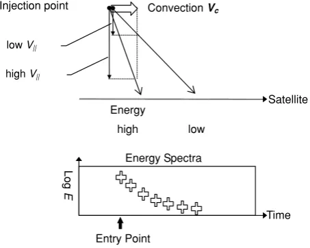
Figure 1 is a schematic diagram illustrating the “ion entry point” that we define in this paper from the data of cusp ion precipitation. Injected ions from the dayside polar cusp are dispersed by magnetospheric convection. Convection oc-curs perpendicular to the field lines, and the convection ve-locity,Vc=Ec×B /B2, is common to all the precipitating
ions (and electrons). However, at the ionospheric altitudes, ions with higher energies are found close to the foot of the injection point because of their shorter travel time along the field line, while ions with lower energies are observed far-ther from the injection point because of their longer travel time, during which ions are convected perpendicular to the field line. Such an energy dispersion structure of injected ions should always be seen except when the convection ve-locity vanishes or when it is exactly perpendicular to the satellite path. The “ion entry point” is defined as the loca-tion where highest energy ions are observed along the satel-lite path. We consider the magnetic field lines threading the “ion entry point” to represent the field lines nearest to the foot of the reconnection line, where the ions are injected into the magnetosphere). In other words, the ion entry point marks the most recently reconnected field lines encountered along the satellite path.
We show four representative cases of the cusp ion en-ergy dispersion for four different IMF conditions in Figs. 2– 5. Cases 1 and 2 occurred in the southern hemisphere
Injection point
Satellite Energy
high
Convection Vc
low
Time
Log
E
Energy Spectra
Entry Point
low V||
high V||
Fig. 1. Definition of “ion entry point” from observation of cusp ion precipitation. The ion entry point is the location where highest energy ions precipitate in the energy dispersion structure of ion precipitation.
for southward and northward IMF conditions, respectively. Cases 3 and 4 occurred in the northern hemisphere for pos-itive and negative IMFByconditions, respectively. The ion
entry points can be clearly identified for each of four cases. The data in Fig. 2 show the case of southward IMF on January 31, 1991 (Case 1). The top two color diagrams give the differential energy flux [eV/cm2/sr/sec/eV] of elec-trons (upper panel) and ions (lower panel). Shown is the maximum differential flux among six pitch angle bins from 0◦ to 180◦. The middle three panels show the integrated flux, average energy, and density of downward precipitat-ing electrons (blue) and ions (green), correspondprecipitat-ing to pitch angles of 90–180 in the southern hemisphere. The bottom panels show the three electric-field components obtained by the double probes. The blue vectors overlaid on theEyplot
indicateE×Bconvection velocities at an altitude of 120 km projected along the field lines; Vx is positive upward
(sunward) andVy is positive toward left (duskward). The
same vectors are plotted along the Akebono orbit projected onto the ionosphere at the bottom of the figure. Akebono traveled poleward near geomagnetic noon in the southern polar region. It encountered the cusp precipitation at lati-tudes of 72–76◦ in the corrected geomagnetic coordinates at 0738–0745 UT. The ion energy was highest at the lat-itude of about 72◦ and decreased with increasing latitude. This flux peak occurred a small distance away from the lo-cation of the energy peak. In addition, we note that the plasma convection obtained from the electric field was di-rected poleward for the corresponding time interval, and the satellite trajectory was almost parallel to the convection di-rection. The hourly values of solar wind parameters were: ion temperature 45,300 K, density 20.4 /cc, velocity 373 km/s, and IMF vector components Bx, By, and Bz,−5.9, −3.7, and−8.0 nT, respectively. It is known that during periods of such a strong southward IMF, a two-cell type convection pattern usually occurs in the polar region, which is consistent with the observed poleward convection near noon. The existence of ion precipitation having a latitudinal energy dispersion within the region of poleward convection is a typical signature for a strong southward IMF.
1
Fig. 2. An example of a cusp ion precipitation event observed in the southern hemisphere for the case of southward IMF on January 31, 1991 (Case 1). The Akebono trajectory is directed poleward near noon. A typical cusp ion precipitation with a clear energy dispersion is recorded, with the highest energy ions precipitating at latitude 72 and energies decreasing poleward. The automatically determined cusp precipitation interval for this case is 0737:56–0744:44 UT.
Figures 4 and 5 show, respectively, the data obtained dur-ing the period of positive IMF By on July 25, 1991 (Case
3) and during the period of negative IMFByon August 6,
1991 (Case 4). In both cases, Akebono traveled in the day-side northern polar region from dawnday-side toward duskday-side.
1
Fig. 3. The same as Fig. 2, but for the northward IMF case on October 5, 1989, observed in the southern hemisphere (Case 2). The satellite trajectory is almost the same as Case 1, but the data show cusp ion precipitation with clear energy dispersion with energies decreasing equatorward. The automatically determined cusp interval is 0825:40–0830:44 UT.
that there is a large difference in the IMFBycomponent
be-tween these two cases. Cusp ion precipitation in Case 3 was observed in the latitudinal range of 78–80◦and in the local time range of 10.4–12.2 MLT (2252–2259 UT). Cusp ion precipitation in Case 4 was observed in the latitudinal range of 76–78◦ and in the local time range of 12.9–13.9 MLT
1
UT 22:35 22:40 22:45 22:50 22:55 23:00 23:05 23:10 23:15 23:20 23:25 23:30 23:35
1991.07.25
(91072522)Akebono
Fig. 4. The same as Fig. 2, but observed in the northern hemisphere for the case of dawnward IMF on July 25, 1991 (Case 3). The satellite trajectory is directed duskward on the dayside. The data show cusp ion precipitation with a clear energy dispersion with energies decreasing duskward. The automatically determined cusp interval is 2251:56–2258:20 UT.
of convection suggested by the ion energy dispersion struc-ture in each case. The occurrence of ion precipitation hav-ing an energy dispersion within the region of east-west con-vection is a typical signature for strong IMF By periods.
The mainly east-west direction of convection around noon is consistent with the three-cell convection pattern observed
for the periods of large IMFBy.
Cases 1 to 4 show that the ion energy dispersion structure can be understood as a spatial structure controlled by IMF. The direction of ion convection around noon strongly de-pends on the sign of IMFByandBzcomponents. Cusp
1
UT 22:10 22:15 22:20 22:25 22:30 22:35 22:40 22:45 22:50 22:55 23:00 23:05 23:10
1991.08.06
(91080622)Akebono
Fig. 5. The same as Fig. 4, but for the case of duskward IMF on August 6, 1991 (Case 4). The satellite trajectory is directed duskward on the dayside. The data show cusp ion precipitation with a clear energy dispersion with energies decreasing dawnward. The automatically determined cusp interval is 2244:28–2251:16 UT.
a few hours of local time in the direction controlled by the signs of IMFByandBz. This dispersion effect makes it
dif-ficult to study the location of the foot of the injection point. Therefore, it would be interesting if we have a more accu-rate estimation of the foot point of the reconnection line. For this purpose, we determined the location of the ion
PASS 91013107
0737 UT ~ 0744 UT
Fig. 6. The 8-sec ion spectrograms for Case 1 (Fig. 2) taken at 0737–0744 UT. Horizontal axis represents pitch-angle (180◦–0◦) of ions in each box. (Ions going upward correspond to 180◦and ions going upward correspond to 0◦because of the southern hemisphere).
Table 1. Automatically determined temporal and spatial (latitude, magnetic local time) ranges of the ion precipitation event, and the determined position of “ion entry point” for Cases 1–4.
Date IMF Event start Event end “Ion entry point”
UT LAT MLT UT LAT MLT LAT MLT
1 910131 Bz− 0737:56 −75.89 12.39 0744:44 −72.35 12.25 −72.43 12.25
2 891005 Bz+ 0825:40 −83.25 12.24 0830:44 −79.32 11.98 −83.25 12.24
3 910725 By− 2251:56 80.23 12.22 2258:20 78.36 10.42 78.36 10.42
4 910806 By+ 2244:28 78.21 12.92 2251:16 76.27 13.95 76.36 13.91
LAT vs IMF Bz
y = 0.7436x + 77.223 R2 = 0.7064
y = 0.6601x + 76.397 R2 = 0.6952
60 65 70 75 80 85 90
-20 -10 0 10 20
IMF Bz (nT)
LAT
IMF By > 0 IMF By < 0 LAT vs IMF By
y = 0.0203x + 79.496 R2 = 0.0016
y = 0.0197x + 73.529 R2 = 0.0014 60
65 70 75 80 85 90
-20 -10 0 10 20
IMF By (nT)
LAT
IMF Bz > 0 IMF Bz < 0
Fig. 7. The IMF dependence of the latitude (LAT) of the ion entry point. The left panel shows the latitude versus IMFByplot. Green points are for the cases of positiveBzand pink points are for the cases of negativeBz. The right panel shows the latitude versus IMFBzplot. Blue points are for the cases of positiveByand red points are for the cases of negativeBy. The colored lines show the regression lines for each IMF polarity.
hand, comparing cases 3 and 4, we see a clear dependence of the local time of the ion entry point on IMFBy. In the
following sections we will investigate the dependence of the location of the ion entry point on the IMF statistically using a large volume of data set obtained by Akebono.
2.3 Cusp event selection
The statistics of cusp-ion precipitation derive from more than 3,000 orbits of Akebono observations from 1989– 1993, for which hourly IMF data were available. We be-lieve that hourly values are appropriate for our correlational study because IMF effects on the magnetosphere require a finite time (of the order of tens of minutes) to establish itself
in the form of convection. We excluded from our statistics the cases where eitherBzorBychanged sign from the
MLT vs IMF Bz
y = 0.0178x + 12.534 R2 = 0.0029
y = -0.0246x + 11.294 R2 = 0.0074 6
8 10 12 14 16 18
-20 -10 0 10 20
IMF Bz (nT)
MLT
IMF By > 0 IMF By < 0 MLT vs IMF By
y = 0.169x + 11.755 R2 = 0.2978
y = 0.0826x + 11.949 R2 = 0.0923 6
8 10 12 14 16 18
-20 -10 0 10 20
IMF By (nT)
MLT
IMF Bz > 0 IMF Bz < 0
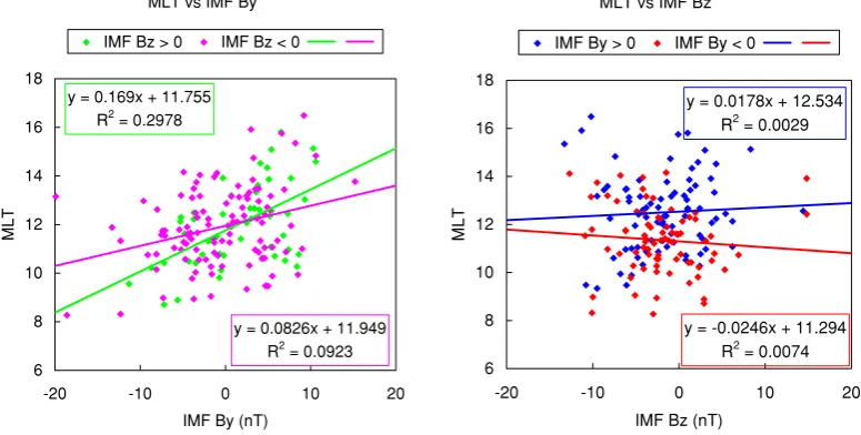
Fig. 8. Dependence of the magnetic local time (MLT) of the ion entry point on IMF, given in the same format as Fig. 7.
Vc-pole vs IMF Bz
y = -0.0488x + 0.1479 R2 = 0.3635
y = -0.0503x + 0.1969 R2 = 0.3011
-4 -3 -2 -1 0 1 2 3 4
-20 -10 0 10 20
IMF Bz (nT)
Vc-pole (km/s)
IMF By > 0 IMF By < 0
Vc-east vs IMF By
y = -0.1201x + 0.3005 R2 = 0.6796
y = -0.1043x + 0.1378 R2 = 0.414
-4 -3 -2 -1 0 1 2 3 4
-20 -10 0 10 20
IMF By (nT)
Vc-east (km/s)
IMF Bz > 0 IMF Bz < 0
Fig. 9. The IMF dependence of the convection flow vectors estimated from the observed electric field: the poleward component of the convection velocity (V p) is plotted against IMFBz (left) and the eastward components (V e) is plotted against IMF By (right). The colors have the same meanings as in Figs. 7 and 8.
the solar wind. These conditions are useful for distinguish-ing cusp from precipitation of magnetospheric origin. The latter two conditions are to avoid weak flux events for which the number of particle counts is close to the background noise level of the detector. Similar conditions have been im-posed by Newell and Meng (1987) for identifying the low-altitude cusp and its neighboring precipitation with DMSP data. For the present study, ion precipitation event is in-cluded in the analysis only when the above conditions were continuously satisfied during a period longer than 32 sec.
After a cusp precipitation event was automatically se-lected with a computer program, we required two additional criteria to be satisfied in order for the event to be included in the analysis. (5) The precipitation shows a clear ion disper-sion signature spanning at least one order of magnitude in energy. (6) The pitch angle-energy dispersion signature is recognized in 8-sec resolution ion data. Condition (5) is em-ployed to make the determination of the “ion entry point”
in the energy dispersion curve easier and more reliable. In order to see the meaning of the condition (6), we show in Fig. 6 examples of 8-sec pitch angle-energy ion spectro-grams for Case 1 (for the time interval of 0737–0744 UT). In each panel, the vertical axis represents ion energy and the horizontal axis represents ion pitch-angle (180◦ for down-ward directed ions and 0◦for upward directed ions). Pan-els are displayed in the order of increasing time. The pres-ence of pitch angle-dependent energy dispersion evidpres-ences that the ions have precipitated through magnetic flux tubes linked to the polar cusp; Burchet al.(1982) explained the pitch-angle energy dispersion in terms of the time-of-flight effect along the field lines assuming that the cusp ion source is narrow. Menietti and Burch (1988) calculated the field-aligned distance of the source to be about 10 Re from the observed point at an altitude of about 20,000 km.
60
00 12
18 06
IMF : By>0, Bz>=0
12 pass , |Kp|=1.9 1 km/s
60
00 12
18 06
IMF : By<0, Bz>=0
14 pass , |Kp|=2.9 1 km/s
60
00 12
18 06
IMF : By>0, Bz<0
26 pass , |Kp|=3.8 1 km/s
60
00 12
18 06
IMF : By<0, Bz<0
27 pass , |Kp|=3.9 1 km/s
NORTH: total 79
60
00 12
18 06
IMF : By>0, Bz>=0
4 pass , |Kp|=2.1 1 km/s
60
00 12
18 06
IMF : By<0, Bz>=0
13 pass , |Kp|=1.8 1 km/s
60
00 12
18 06
IMF : By>0, Bz<0
21 pass , |Kp|=3.8 1 km/s
60
00 12
18 06
IMF : By<0, Bz<0
20 pass , |Kp|=3.7 1 km/s
SOUTH: total 58
Fig. 10. Convection velocity vectors are plotted in such a way that they start from the observed positions of entry points (circles). Data for the northern hemisphere are shown on the left and data for the southern hemisphere on the right.
the northern hemisphere), and determined the location of the ion entry point for each event. Note that electron data were not used to identify the entry point because the energy range of cusp electron precipitation (about 100 eV on aver-age) is close to that of photoelectrons (<70 eV). The time intervals and the spatial ranges of ion precipitation events as determined by the above criteria for Cases 1–4 are listed in Table 1.
2.4 Statistics
We investigated the relationship between IMF conditions (in particular,Y andZcomponents) and the location of ion entry point for 159 cusp precipitation events.
Let us start with the latitude (LAT) and magnetic local time (MLT) of the entry point plotted in Figs. 7 and 8, re-spectively. The left panel of each figure shows the latitudes plotted against IMFBy; the green points are for positiveBz,
and the pink ones are for negativeBz. The right panels show
positiveBy, and red ones are for negativeBy. The colored
lines represent the linear regression lines for different IMF conditions.
The comparison of Cases 1 to 4 we made earlier indicated that the entry point is displaced in the longitudinal direction by IMF By and in the latitudinal direction by IMF Bz.
Since the longitudinal effect of IMF By in the northern
hemisphere is found to be opposite to that in the southern hemisphere, the southern and northern hemisphere events are plotted with the sign of IMFByreversed and the mirror
image of the satellite path is adopted with respect to the noon-midnight plane for the southern hemisphere events.
Figure 7 clearly shows that there is a clear linear relation-ship between the latitude of the ion entry point and IMFBz
(see the right panel) but no relationship for IMFBy(see the
left panel). As a mater of fact, the regression lines shown in the right panel are almost the same for positive and neg-ative By. We conclude that IMF By component does not
influence the latitudinal position of the ion entry point. On the other hand, Fig. 8 shows that the MLT (magnetic local time) of the ion entry point is related with IMF By;
the entry point tends to occur at a later local time for more positive IMFBy. Both two panels show that the MLT of the
ion entry point has a weakBzdependence in such a way that
the dependence onByis larger for northward IMF than for
southward IMF. This effect is addressed in the discussion section.
Note that the number of events for positive IMF Bz is
less than for negative IMF Bz. We suggest that this is due
to one of our criteria used to select cusp ion precipitation, i.e. the condition that the energy dispersion should cover at least one order of magnitude in energy. We found that a significant portion of the cusp ion precipitation events for northward IMF does not show a clear energy dispersion and hence does not satisfy this condition.
2.5 Convection with cusp precipitation
Each of Case 1–4 shows clear IMF ByandBz effects on
convection flows accompanied with cusp precipitation. The direction of convection flows projected onto the 120 km al-titude level obtained from the electric field data is consis-tent with that predicted from the spatial energy dispersion of cusp ion precipitation. Figures 9 and 10 show the con-vection flows averaged over each event obtained from the 8-sec electric field data. In Fig. 9, the poleward compo-nents (Vp) of the convection velocity is plotted against IMF
Bz (left) and the eastward components (Ve) of the
convec-tion velocity is plotted against IMFBy(right). The meaning
of colors is the same as Figs. 7 and 8. Figure 10 shows the same data in the form of the two-dimensional polar coordi-nate maps; northern hemisphere is shown to the left and the southern hemisphere is shown to the right. The small cir-cles indicate the locations of the ion entry points and the at-tached vectors represent the convection velocity vectors for the corresponding events. We note that the electric field data were not available for some of the selected events so that the number of events (137) shown in Figs. 9 and 10 are less than that shown in Figs. 7 and 8. It is found from these plots that (1) the convection velocity tends to have a large azimuthal component, (2) the azimuthal component is almost linearly related to IMF By, (3) the cases of equatorward
convec-Fig. 11. Schematic diagram showing the difference of magnetic field con-figuration around the polar cusp between the northward and southward IMF cases. The ion entry point is regarded as the poleward (equator-ward) edge of the polar cusp during northward (south(equator-ward) IMF.
tion are few and appear only for strong northward IMF, and (4) poleward convection is observed for southward IMF and even for northward IMF in some cases.
3.
Discussion
Since the ion entry point is probably associated with the magnetic foot point of the dayside reconnection line, we ex-amine the location of the ion entry point and its dependence on IMF in order to obtain information about the dayside re-connection sites.
3.1 Latitudinal displacement
The ion entry point is regarded as the point nearest to the foot point of the separatrix of reconnected field lines, so that its latitudinal displacement is attributed to a property of the high-latitude reconnection when IMFBz>0 and to a
prop-erty of the low-latitude reconnection whenBz <0. In other
words, the ion entry point for IMFBz > 0 is expected to
represent the poleward edge of the polar cusp and that for IMFBz <0 is expected to represent its equatorward edge.
Northward IMF and By > 0 Southward IMF and By > 0
6 18
12 18
12 6
Fig. 12. Schematic diagrams showing the region of the ion entry point (solid areas) and the assumed convection flow direction (white arrows) for dominantly positive (negative) IMFByin the northern (southern) hemisphere.
Fig. 13. The number of ion entry points as a function of MLT, the upper panel for northward IMF and the lower panel for southward IMF. For each panel, black lines show the cases with positive IMFByand grey lines with negative IMFBy.
IMF conditions. The relationship between the latitudinal position of the ion entry point and convection direction is easily understood in this figure. For southward IMF, terres-trial field lines are peeled off from the low-latitude magne-topause by the reconnection process occurring on the closed filed lines, so that the ion entry point moves toward lower latitudes, while the convection is directed poleward. On the other hand, for northward IMF, high-latitude reconnection occurs at the position tailward of the cusp so that the high-latitude field lines are peeled off and the ion entry point moves poleward while the convection is directed equator-ward. The white arrows in Fig. 11 indicate the direction of convection.
Results shown in the right panel of Fig. 7 suggest that the dependence of the the ion entry point on Bz can be
expressed by a single linear regression line irrespective of theByandBzsigns. The best-fit regression formula for the
distribution of all the 159 points is
L AT[deg]=0.71Bz[nT]+76.8. (1)
The correlation coefficient is 0.83. Note that our analysis is an average over different geomagnetic dipole tilt angles, and still a high degree of correlation has been obtained. The linear dependence suggests that the reconnection rate for the southward and northward IMF is not much different from each other. The continuity of the distribution of data points between the northward and southwardBzranges (see
the right panel of Fig. 7) suggests that there is no wide gap separating the poleward and equatorward edges of the cusp. This would imply that the latitudinal width of the cusp is narrow, but it would be difficult to quantify the result at this moment.
In Paper 1 we already reported the presence of a good correlation between the latitude of ion entry point and IMF Bz. We found that the solar wind velocity weakly but clearly
affects the latitudinal displacement of the ion entry point. It should be noted that the Vsw effect is not in the form
of the solar wind dynamic pressure but in the form of the solar wind electric field (E = −Vsw ×BIMF) which acts
to peel-off the terrestrial field lines. The dynamic pressure of the solar wind, ρVs2w, directly controls the size of the
magnetosphere but not the cusp latitude (see Sibecket al., 1991, and Shueet al., 1997, for statistical analyses). Paper 1 also indicated that latitudinal saturation seems to occur at about 65◦and 85◦for electric fields exceeding±5 mV/m.
Newellet al.(1989) reported the IMF effect on the po-sition of the dayside cusp precipitation on the basis of data taken by DMSP satellites (at an altitude of 840 km). How-ever, in Newell’s analysis, the energy dispersed nature of ion precipitation is not explicitly taken into account in the analysis of cusp location. They used for their analysis the position of the “cusp proper” where the number flux of ion precipitation was highest. They deduced different regres-sion lines for different polarities of IMF Bz. On the other
hand, our result suggests that the dependence can be ex-pressed by a single regression line for entire range of IMF Bz. It is interesting that our regression line for the entire
range of IMF Bz is very close to Newell’s regression line
for southward IMF, i.e., LAT[deg] = 0.76Bz[nT]+77.0,
but we regard the close similarity to be coincidental. It is also interesting to note that the correlation coefficient ob-tained from our analysis is significantly higher than that of Newell (0.70 for the southward IMF) in spite of the fact that our result includes both southward and northwardBzcases.
Z
Y
(duskward) Duskward IMF
(By > 0) Convection
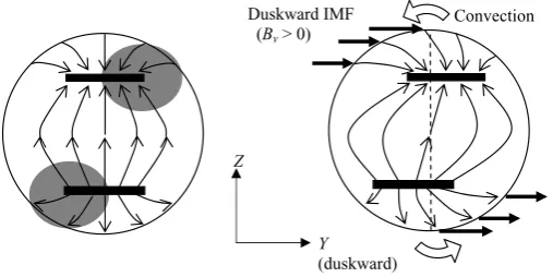
Fig. 14. Magnetic field line configuration on the dayside magnetopause as viewed from the sun. Undistorted magnetic field lines for the case of no IMF is shown in the left panel and a field line configuration distorted by the presence of duskward IMF (positiveBy) is shown in the right panel. The solid areas indicate the polar cusp, whose magnetic foot print would correspond to the ion entry points shown in Fig. 12.
of the cusp precipitation by introducing the concept of the ion entry point defined as the high-energy edge of the cusp ion precipitation. This definition is based on a theoretical consideration that it would represent the point closest to the foot point of the reconnection line along the satellite path. A high correlation coefficient obtained from our analysis may suggest that the latitudinal displacement of the ion en-try point really reflects the latitudinal change of the starting point of reconnection and that our method worked well to remove the ambiguity due to the energy dispersion effects. Freyet al. (2002, 2003) referred to the Newell’s result in the study of cusp proton aurora for southward IMF and not for northward IMF. Our result suggests that a single rela-tionship between the cusp position and IMFBz applies for
both northward and southward polarities.
3.2 Longitudinal displacement
Dayside convection is directed toward the pre-noon (post-noon) sector when IMF By is positive (negative) in
the northern hemisphere (Heelis, 1984; Goslinget al., 1990; etc.). Our results shown in Figs. 9 and 10 agree with these past studies. On the other hand, we found that the ion entry point defined in our paper shifts in the direction opposite to the convection direction, as shown in Fig. 8.
Figure 12 schematically shows the probable regions of the entry point (shaded areas) and the direction of the con-vection flow (white arrows) for dominantly positive (neg-ative) IMF By in the northern (southern) hemisphere (after
Basinskaet al., 2002). The right and left diagrams represent the cases for the negative and positive IMFBz, respectively.
Note that for the other polarity of By, i.e. for the cases of
negative (positive) IMFByin the northern (southern)
hemi-sphere, the whole diagram becomes a mirror image about the noon meridian of Fig. 12. Our result suggests that the Bydependence of the ion entry point is consistent with the
picture presented in Fig. 12. Our result also suggests that the ion entry point may be distributed in a longitudinally wide area, as is consistent with Fig. 12, since there is a large degree of scatter in magnetic local time plotted as a function of IMFByin Fig. 8.
We noted earlier that the magnitude of the IMFByeffect
on the azimuthal position of the ion entry point is differ-ent between the southward and northward IMF cases (see Fig. 8). To clarify this difference, Fig. 13 shows the MLT
distribution of ion entry points for different polarities of IMFBy for northward (upper panel) and southward (lower
panel) IMF conditions. In each panel, black lines are for positiveByand grey lines are for negativeBy. Colored
ver-tical dashed lines in each panel indicate the average MLT position of the entry point for each IMF polarities. We can clearly see that the magnitude of the local-time shift of ion entry point induced by IMF By is larger for northwardBz
than for southwardBz. In order to discuss the reason for this
tendency, magnetic field line configuration on the dayside magnetopause is schematically shown in Fig. 14, as viewed from the sun (cf., Crookeret al., 1987; Stasiewicz, 1991; Fuselieret al., 2003). Undistorted magnetic field lines for the case of no IMF is shown on the left and a field line configuration distorted by the presence of positive IMFBy
is shown on the right. The shaded areas in the left panel indicate the positions whose magnetic foot print would cor-respond to the region of ion entry point shown in Fig. 12. (Note that Fig. 12 is for the northern hemisphere.)
The sense of the By-related shift of the polar cusp has
been interpreted in the literature in the following way. Magnetospheric magnetic field lines on the magnetopause around the polar cusp have diverse directions, so that it is easy for them to satisfy the anti-parallel field condition, which has been proposed by some researchers to be a neces-sary condition for magnetic reconnection. When IMFByis
positive, the shadowed areas in the left diagram are a candi-date for the site of anti-parallel reconnection. In the north-ern hemisphere, for example, the shadowed area is on the duskside of the polar cusp, and the magnetic field lines on the duskside are peeled-off, and therefore the ion entry point moves toward dusk. This movement of the ion entry point is opposite to the convection direction shown by white arrows in Fig. 12 (and also shown in the right panel of Fig. 14), and is consistent with our statistics.
In conclusion, our result on the IMF By dependence of
ion entry point is consistent with the concept of anti-parallel reconnection. However, we should point out an important possibility that our result is also consistent with the concept of component merging. Crooker et al.(1997) studied on high latitude merging sites during periods of large IMFBy
of Fig. 14 shows the distorted magnetospheric field lines on the magnetopause based on their simulation. The magneto-spheric magnetic field lines are distorted because the IMF By component penetrates into the magnetosphere as a
re-sult of reconnection. We should point out that the sufficient condition for this kind of field line distortion is that IMF Bypenetrates into the magnetosphere, and the condition is
not related to the question of whether the anti-parallel con-dition or component merging concon-dition is satisfied at the reconnection point. Once the magnetospheric field lines are distorted in the way depicted in the right panel of Fig. 14, it would be a easy matter to see that the foot point of the dayside low latitude field lines, on which the component merging is assumed to occur, is also shifted toward dusk in the northern hemisphere and toward dawn in the south-ern hemisphere, in a way similar to the case of anti-parallel reconnection.
The above discussion implies that our results (as well as other similar results in literature) do not discriminate be-tween anti-parallel and component merging. We actually conjecture that reconnection can occur both on the low-latitude field lines and on the cusp field lines when IMF Bz is close to zero. The probability of high-latitude
re-connection would become higher for northward IMF and the probability of low-latitude reconnection would become higher for southward IMF. The strongerBydependence of
the MLT position of the ion entry point for northward IMF would then mean that the By dependence of the position
of the anti-parallel merging site around the cusp is stronger than the field line distortion effect associated with the low-latitude reconnection. We should also consider the fact that the low latitude reconnection line for the case of southward IMF is expected to be extended over a wide range of MLT so that the local time position of the ion entry point may have a large scatter, as is consistent with the result shown in Fig. 8.
4.
Summary
From the analysis of ion precipitation events observed by the Akebono satellite, we have statistically investigated lati-tudinal and longilati-tudinal displacements of cusp precipitation controlled by IMF. We introduced the concept of “ion entry point” which is defined to be the point where the precipita-tion ion energy was the maximum along the satellite path. The ion entry point is interpreted to be the point nearest to the magnetic foot point of the dayside magnetic reconnec-tion line along the satellite path.
Our analysis showed that the location of the ion entry point has a strong dependence on the sign and magnitude of IMF By and Bz. By and Bz have almost orthogonal
effects on the location of the entry point, with the latitudinal displacement linearly related to Bz, and the longitudinal
displacement linearly related toBy. We have found that the
Bzdependence of the ion entry point can be represented by
a single regression line for entire range of Bz irrespective
of its north/south polarity. We have also found that the By dependence is larger for positive Bz than for negative
Bz. The distribution of ion entry points for positive IMFBy
is almost a mirror image of that for negative IMF Bywith
respect to the noon-midnight meridian plane. We discussed
the dependence of the ion entry point on the IMF from the viewpoint of where magnetopause reconnection (merging) occurs on the dayside magnetosphere and how the field lines are distorted by the reconnection process. We conclude that the observed dependence of the ion entry point on IMF By is consistent with both the anti-parallel and component
merging models of the dayside reconnection.
Acknowledgments. The solar wind and IMF data used in this analysis were provided by NSSDC.
References
Aparicio, B., B, Thelin, and R. Lundin, The polar cusp from a particle point of view: A statistical study based on Viking data,J. Geophys. Res.,96, 14023–14031, 1991.
Asai, K., K. Maezawa, N. Kaya, and T. Mukai, Latitudinal displacement of cusp ion precipitation: Akebono observations,Adv. Space Res.,23, 1761–1764, 1999.
Basinska, E. M., W. J. Burke, N. C. Maynard, W. J. Hughes, J. D. Winning-ham, and W. B. Hanson, Small-scale electrodynamics of the cusp with northward Interplanetary Magnetic Field,J. Geophys. Res.,97, 6369– 6379, 1992.
Burch, J. L., P. H. Reiff, R. A. Heelis, J. D. Winningham, W. B. Hanson, C. Gurgiolo, J. D. Menietti, R. A. Hoffman, and J. N. Barfield, Plasma injection and transport in the mid-altitude polar cusp,Geophys. Res. Lett.,9, 921–924, 1982.
Chandler, M. O., S. A. Fuselier, M. Lockwood, and T. E. Moore, Evidence of component merging equatorward of the cusp,J. Geophys. Res.,104, 22,623–22,634, 1999.
Cowley, S. W. H., The couses of convection in the Earth’s magnetosphere: A review of developments during IMS,Rev. Geophys.,20, 531–565, 1982.
Cowley, S. W. H., J. P. Morelli, and M. Lockwood, Dependence of convec-tive flows and particle precipitation in the high-latitude dayside iono-sphere on the X and Y components of the interplanetary magnetic field,
J. Geophys. Res.,96, 5557–5564, 1991.
Crooker, N. U., J. Berchem, and C. T. Russell, Cusp displacement at the magnetopause for large IMF Y component,J. Geophys. Res.,92, 13467–13471, 1987.
Crooker, N. U., J. G. Lyon, and J. A. Fedder, MHD model merging with IMF By: Lobe cells, sunward polar cap convection, and overdraped lobes,J. Geophys. Res.,103, 9143–9152, 1998.
Farrugia, C. J., P. E. Sandholt, R. B. Torbert, and N. Østgaard, Temporal and spatial aspects of the cusp inferred from local and global ground-and space-based observations in a case study,J. Geophys. Res.,109, A04209, 2004.
Frey, H. U., S. B. Mende, T. J. Immel, S. A. Fuselier, E. S. Claflin, J.-C. G´erard, and B. Hubert, Proton aurora in the cusp,J. Geophys. Res.,107, 1091, 2002.
Frey, H. U., S. B. Mende, S. A. Fuselier, T. J. Immel, and N. Østgaard, Proton aurora in the cusp during southward IMF,J. Geophys. Res.,108, 1277, 2003.
Fuselier, S. A., H. U. Frey, K. J. Trattner, S. B. Mende, and J. L. Burch, Cusp aurora dependence on interplanetary magnetic fieldBz,J.
Geo-phys. Res.,107, 1111, 2002.
Fuselier, S. A., S. B. Mende, T. E. Moore, H. U. Frey, S. M. Petrinec, E. S. Claflin, and M. R. Collier, Cusp dynamics and ionospheric outflow,
Space Science Reviews,109, 285–312, 2003.
Gosling, J. T., M. F. Thomsen, S. J. Bame, R. C. Elphic, and C. T. Russell, Plasma flow reversals at the dayside magnetopause and the origin of asymmetric polar cap convection, J. Geophys. Res., 95, 8073–8084, 1990.
Hakura, Y., Tables and maps of geomagnetic coordinates corrected by the higher order spherical harmonic terms,Rep. Ionos. Space Res. Japan, 19, 121–157, 1965.
Hayakawa, H.,et al., Electric field measurement on the Akebono (EXOS-D) satellite,J. Geomag. Geoelectr.,42, 371–384, 1990.
Heelis, R. A., The effects of interplanetary magnetic field orientation on dayside high-latitude ionospheric convection,J. Geophys. Res.,89, 2873–2880, 1984.
Karlson, K. A., M. Oieroset, J. Moen, and P. E. Sandholt, A statistical study of flux transfer event signatures in the dayside aurora: The IMF
1996.
Kremser, G. and R. Lundin, Average spatial distributions of energetic particles in the midaltitude cusp/cleft region observed by Viking,J. Geophys. Res.,95, 5753–5766, 1990.
Lockwood, M., Relationship of dayside precipitation to the open-closed separatrix and the pattern of convection flow,J. Geophys. Res.,102, 17475–17487, 1997.
Lockwood, M., S. W. Cowley, P. E. Sandholt, and U. P. Lovhaug, Causes of plasma flow bursts and dayside auroral transients: an evaluation of two models invoking reconnection pulses and chaned in the Y component of the magnetosheath field,J. Geophys. Res.,100, 7613–7626, 1995. Lockwood, M., S. W. H. Cowley, and T. G. Onsager, Ion acceleration at
both the interior and exterior Alfven waves associated with the magne-topause reconnection site: Signatures in cusp precipitation,J. Geophys. Res.,101, 21501–21513, 1996.
Maezawa, K., Magnetospheric convection induced by the positive and negative Z components of the interplanetary magnetic field: quantitative analysis using polar cap magnetic records,J. Geophys. Res.,81, 2289– 2303, 1976.
Maynard, N. C., W. J. Burke, P. E. Sandholt, J. Moen, D. M. Ober, M. Lester, D. R. Weimer, and A. Egeland, Observations of simultaneous effects of merging in both hemispheres,J. Geophys. Res.,106, 24551– 24578, 2001.
Menietti, J. D. and J. L. Burch, Spatial extent of the plasma injection region in the cusp-magnetosheath interface,J. Geophys. Res.,93, 105–113, 1988.
Mukai, T., N. Kaya, E. Sagawa, M. Hirahara, W. Miyake, T. Obara, H. Miyaoka, S. Machida, H. Yamagishi, M. Ejiri, H. Matsumoto, and T. Itoh, Low energy charged particle observation in the “auroral” magne-tosphere: First results from Akebono (EXOS-D) satellite,J. Geomag. Geoelectr.,42, 479–496, 1990.
Newell, P. T. and C.-I. Meng, Cusp width andBz: Observations and con-ceptual model,J. Geophys. Res.,92, 13673–13678, 1987.
Newell, P. T. and C.-I. Meng, The cusp and the cleft/boundary layer: Low-altitude identification and statistical local time variation,J. Geophys. Res.,93, 14549–14556, 1988.
Newell, P. T., C.-I. Meng, D. G. Sibeck, and R. Lepping, Some low-altitude cusp dependencies on the interplanetary magnetic field,J. Geophys. Res.,94, 8921–8927, 1989.
Newell, P. T., W. J. Burke, C.-I. Meng, E. R. Sanches, and M. E. Greenspan, Identification and observations of the plasma mantle at low altitude,J. Geophys. Res.,96, 35–45, 1991a.
Newell, P. T., W. J. Burke, C.-I. Meng, E. R. Sanches, M. E. Greenspan, and C. R. Clauer, The low-latitude boundary layer and the boundary plasma sheet at low altitude: Prenoon precipitation regions and convec-tion reversal boundaries,J. Geophys. Res.,96, 21013–21023, 1991b.
Onsager, T. G., C. A. Kletzing, J. B. Austin, and H. MacKiernan, Model of magnetosheath plasma in the magnetosphere: Cusp and mantle particles at low-altitudes,Geophys. Res. Let.,20, 479–482, 1993.
Onsager, T. G., S.-W. Chang, J. D. Perez, J. B. Austin, and L. X. Janoo, Low-altitude observations and modeling of quasi-steady magnetopause reconnection,J. Geophys. Res.,100, 11831–11843, 1995.
Onsager, T. G., J. D. Scudder, M. Lockwood, and C. T. Russell, Reconnec-tion at the high-latitude magnetopause during northward interplanetary magnetic field conditions,J. Geophys. Res.,106, 25467–25488, 2001. Reiff, P. H., T. W. Hill, and J. L. Burch, Solar wind plasma injection at the
dayside magnetospheric cusp,J. Geophys. Res.,82, 479–491, 1977. Ridley, A. J., G. Lu, C. R. Clauer, and V. O. Papitashvili, A statistical
study of the ionospheric convection response to changing interplanetary magnetic field conditions using the assimilative mapping of ionospheric electrodynamics technique,J. Geophys. Res.,103, 4023–4040, 1998. Rosenbauer, H., H. Grunwaldt, M. D. Montgomery, G. Paschmann, and
N. Sckopke, Heos 2 plasma observations in the distant polar magneto-sphere: the plasma mantle,J. Geophys. Res.,80, 2723–2737, 1975. Sandholt, P. E. and C. J. Farrugia, Does the aurora provide evidence for
the occurrence of antiparallel magnetopause reconnection?,J. Geophys. Res.,108, 1466, 2003.
Shue, J.-H., J. K. Chao, H. C. Fu, C. T. Russell, P. Song, K. K. Khurana, and H. J. Singer, A new functional form to study the solar wind control of the magnetopause size and shape,J. Geophys. Res.,102, 9497–9511, 1997.
Sibeck, D. G., R. E. Lopez, and E. C. Roelof, Solar wind control of the magnetopause shape, location, and motion,J. Geophys. Res.,96, 5489– 5495, 1991.
Stasiewicz, K., A global model of gyroviscous field line merging at the magnetopause,J. Geophys. Res.,96, 77–86, 1991.
Stubbs, T. J., P. J. Cargill, M. Lockwood, M. Grande, B. J. Kellett, and C. H. Perry, Extended cusp-like regions and their dependence on the Polar orbit, seasonal variations, and interplanetary conditions,J. Geophys. Res.,109, A09210, 2004.
Twitty, C., T. D. Phan, G. Paschmann, B. Lavraud, H. R`eme, and M. Dunlop, Cluster survey of cusp reconnection and its IMF dependence,
Geophys. Res. Lett.,31, L19808, 2004.
Woch, J. and R. Lundin, Magnetosheath plasma precipitation in the polar cusp and its control by the interplanetary magnetic field,J. Geophys. Res.,97, 1421–1430, 1992.