ABSTRACT
BJERKAAS, JAMES KEVIN. Modeling Ground Sensor Acquisitions of Low Earth Orbit Objects. (Under the direction of Professor Thom J. Hodgson).
The United States Strategic Command (STRATCOM) utilizes a sensor network to
accomplish several of its missions. These missions include missile defense, missile warning, intelligence collection, and space surveillance. For the task of space surveillance, the
locations of all man-made satellites, as well as debris formed by the collisions of these satellites, is of great interest to the United States.
Previous work has focused on assigning the various sensors in the sensor network to the separate tasks required. This thesis focuses on developing a simulation to learn more about the dynamic interactions between the sensors and the constantly moving orbiting field of satellites and debris.
The stochastic model developed shows over time what happens to the knowledge of the objects in Low Earth Orbit (LEO) when the sensors assigned to tracking their progress are changed. When sensors are reassigned from space surveillance to another task, the
Modeling Ground Sensor Acquisitions of Low Earth Orbit Objects
by
James Kevin Bjerkaas
A thesis submitted to the Graduate Faculty of North Carolina State University
in partial fulfillment of the requirements for the degree of
Master of Science
Operations Research
Raleigh, North Carolina 2010
APPROVED BY:
_______________________________ ______________________________
Thom J. Hodgson Russell E. King
BIOGRAPHY
James Kevin Bjerkaas was born in Urbana, Illinois in 1970. He attended University of Maryland at College Park and graduated in May 1993 with a Bachelor of Science in Mathematics and a Bachelor of Science in Mathematics Education. After Graduation, he began Basic Combat Training at Fort Leonard Wood, Missouri, where he began his training as a Personnel Administration Assistant in the United States Army Reserve. After serving four years in the United States Army Reserves, he was commissioned as a Second Lieutenant in the United States Army in 1997 through Officer Candidate School (OCS) at Fort Benning, Georgia. He was branched Engineers and returned to Fort Leonard Wood, Missouri to begin his military officer education as a combat engineer.
Rolla and a Master of Science Degree in Industrial Engineering from New Mexico State University in Las Cruces, New Mexico.
James currently holds the rank of Major in the United States Army, and upon graduation, will serve as a mathematics instructor at the United States Military Academy at West Point, New York.
ACKNOWLEDGEMENTS
I would like to recognize and express my appreciation to the following people for their help and support to me while I worked on this thesis.
My wife Julie
My parents and brothers
Derek Tharaldson
TABLE OF CONTENTS
LIST OF TABLES ... vii
LIST OF FIGURES ... viii
1 INTRODUCTION ... 1
1.1 Background ... 1
1.2 Problem ... 2
1.3 Assumptions and Limitations ... 3
1.4 Overview ... 6
2 LITERATURE REVIEW ... 7
2.1 Current Models ... 7
3 MODEL ... 8
3.1 Overall Model Structure ... 9
3.2 Step One: Initialization... 10
3.2.1 Generate Positions for Objects in Low Earth Orbit (LEO)... 11
3.2.2 Generate Positions for Sensors ... 25
3.2.3 Initialize Object Lists ... 29
3.3 Step Two: Increment Time ... 30
3.4 Step Three: Actions at each Time Step ... 30
3.4.1 Update Positions for Objects in Orbit and Sensors ... 30
3.4.2 Calculate Detections of Objects in Orbit by Sensors ... 32
3.4.3 Update Known, Unknown, and Update Lists ... 34
3.5 Simulation Input ... 35
3.5.1 Orbiting Objects Data ... 35
3.5.2 Sensor Data ... 36
3.5.3 Simulation Parameters ... 37
3.6 Simulation Output ... 37
4 EXPERIMENTATION ... 38
4.1 Parameter Selection ... 39
4.1.3 Probability of Detection for an Object within a Radar‟s Field of View ... 45
4.1.4 Movement Times between Object Lists ... 46
4.2 Test Runs ... 49
4.2.1 Demonstration of Steady State Behavior ... 50
4.2.2 Demonstration of Sensor Changes ... 51
4.2.3 Demonstration of Sensor Changes with Actual Data for Objects... 52
5 FUTURE RESEARCH ... 54
5.1 Constant Velocity ... 54
5.2 Additional Sensor Types ... 55
5.3 Orbital Perturbations ... 55
5.3.1 Orbital Perturbations due to the Non-Spherical Shape of the Earth ... 55
5.4 Geographical Locations for Additional Sensors ... 57
REFERENCES ... 58
LIST OF TABLES
Table 3.1. Orbital Parameters for International Space Station ... 13
Table 3.2. XY Coordinates for ISS within Orbital Plane... 15
Table 3.3. XY Coordinates for ISS within Orbital Plane adjusted for Argument of the Perigee ... 19
Table 3.4. XYZ Coordinates for ISS with Adjustment for Inclination ... 21
Table 3.5. XYZ Coordinates for ISS with Adjustment for Right Ascension of the Ascending Node ... 23
Table 3.6. XYZ Coordinates for ISS with time indexing... 25
Table 3.7. Sensor Positions with a Latitude of 30 degrees ... 29
Table 3.8. Phased Array Radar Locations Used ... 36
Table 4.1. Interpolation Error by Number of Partitions... 43
LIST OF FIGURES
Figure 3.1. Simulation Structure ... 10
Figure 3.2. International Space Station Two-Line Elements ... 12
Figure 3.3. Elliptical Parameters ... 14
Figure 3.4. Graphical Representation of ISS Orbit within Orbital Plane ... 16
Figure 3.5. Argument of the Periapsis ... 18
Figure 3.6. Graphical Representation of ISS Orbit within Orbital Plane with Adjustment for Argument of the Perigee ... 19
Figure 3.7. Inclination ... 20
Figure 3.8. Graphical Representation of ISS Orbit with Adjustment for Inclination ... 21
Figure 3.9. Right Ascension of the Ascending Node... 22
Figure 3.10. Graphical Representation of ISS Orbit with Adjustment for Right Ascension of the Ascending Node ... 24
Figure 3.11. Sensor Positions with a Latitude of 30 degrees ... 28
Figure 3.12. Object Lists State Diagram ... 34
Figure 3.13. Sample Simulation Output ... 38
Figure 4.1. Possible Detections by Orbit Partitions ... 40
Figure 4.6. Simulation Results for a Lapse Time of 0.5 Days ... 47
Figure 4.7. Simulation Results for a Lapse Time of 0.25 Days ... 48
Figure 4.8. Simulation Results for a Lapse Time of 0.75 Days ... 49
Figure 4.9. Object Lists Over Time ... 51
Figure 4.10. Object Lists over Time with Subtraction of Sensor ... 52
1 INTRODUCTION
1.1 Background
Two recent events have demonstrated the importance of tracking debris in orbit around the Earth. In January 2007 China conducted an anti-satellite test (Fengyn-1C), and in February 2009 two satellites, Iridium 33 and Cosmos 2251, collided 490 miles (790 kilometers) above the surface of the Earth. These two events created approximately 5000 objects of debris over 10 centimeters in diameter in Low Earth Orbit (LEO), increasing the number of objects tracked by the National Aeronautics and Space Administration (NASA) Space Debris
program by about 50%. (Liou, 2010) This increase in debris makes it increasingly likely that man made satellites will suffer collisions during their orbit around the Earth. In addition, these objects pose risks to manned vehicles in orbit, including the International Space Station.
monitoring and collecting information on all man-made objects in orbit around Earth. From this information they produce a satellite catalog, “used by predictive orbital analysis tools to anticipate satellite threats and mission opportunities for friendly, adversary, and third party-assets.” (3-14, 2009)
Previous work has been conducted in allocating sensors to this task, as well as other tasks such as missile defense, missile warning, and intelligence collection. Dulin developed a heuristic method for determining an optimal allocation of these sensors to their tasks. (Dulin, 2009) In his research, he treated space surveillance as a secondary task, and considered only the probability of success in these tasks. The interaction between sensors and objects in orbit was considered static, while in reality it is a dynamic system. Dulin identified the need to model this task of space surveillance as a dynamic system to achieve a greater level of precision in the overall model. Subsequent work will update Dulin‟s heuristic with a dynamic representation of this task of Space Surveillance. In support of this ongoing research, this thesis provides a simulation for modeling this task of Space Surveillance with greater fidelity and providing insight into the behavior of this dynamic system when sensors are removed or added to the network.
1.2 Problem
range in size from small bolts to large man-made satellites, is non-trivial. Of particular interest is an understanding of what happens to the knowledge of these objects when one or more sensors are reassigned from the task of monitoring the objects to another higher priority task. The questions of interest are: 1) What is the steady state of the system when all sensors are focused on tracking the objects in orbit, 2) What happens to this steady state when one or more sensors are removed. In addition, 2a) what is the new steady state, and 2b) How long does it take to reach this new state? The steady state of the system is defined as the long run average values of what is known about the objects in orbit. For example, with three sensors working to track objects in orbit, how many objects, on average, do they have data on from recent detections.
The simulation represents the movement of these objects in orbit in and out of the acquisition range of the sensors; the acquisition of these objects by the sensors when they are in range of the sensors; and the loss of individual sensors and the effect on the overall system.
1.3 Assumptions and Limitations
1.3.1.1 Perturbations to Orbits due to Non-Spherical Shape of the Earth
where the object is closest to the Earth along its orbit, changes due to the shape of the Earth. For this simulation, the exact positions of objects are not required. The emphasis of the simulation is on the ability to track objects in LEO, not the exact locations of these objects. Ideally, the positions should be simulated as accurately as possible, however, because of run time considerations these perturbations are ignored. This topic is covered in more depth in Chapter 5 Future Research.
1.3.1.2 Perturbations to Orbits due to other Factors
Other perturbations to the orbits around the Earth are also ignored. These include the gravitational forces of other objects, such as the Moon and the Sun, and atmospheric conditions such as atmospheric drag and solar winds. These perturbations have less of an impact on the orbits than the perturbations due to the shape of the Earth. (Capderou, 2005)
1.3.1.3 Galilean Frame of Reference
The simulation assumes a Galilean frame of reference for the orbits in question. This means that the frame of reference is fixed with the origin at the Earth‟s center, the Z axis oriented along the line running from the North to South Pole, and the plane formed by the X and Y axes lies along the equatorial plane of the Earth, with the X axis oriented towards the Vernal Equinox.
1.3.1.4 Constant Velocity
shortens run-time. For the sample set of 4880 object in orbit used for this thesis, 4803 have eccentricities less than 0.1, where an eccentricity of 0 represents a circular orbit.
1.3.1.5 Sensors Modeled
The sensors modeled are assumed to have similar characteristics to the Phased Array radar. Exact operating data was not available, so approximate ranges and failure rates were
parameterized. In addition, the Space Fence was not modeled. The Space Fence is a set of transmitters and receivers along 33 degrees North latitude which detect any objects passing over the United States.
1.3.1.6 Sensors not Modeled
Long range sensors, such as optical telescopes, were not modeled. The focus of the model was on sensors focused on LEO, which are defined for purposes of this simulation as any orbit with an altitude of less than 2000 km from the surface of the Earth. In addition, passive receivers, which track transmissions from functioning man-made satellites, are not modeled.
1.3.1.7 Time Dependency of Object Lists
orbit, or a maneuverable satellite changing course, this simulation deals with only changes due to elapsed time.
1.3.1.8 Classification of Parameters
In addition, some information, such as the reliability of the radars, and the schedules for which sensors are used when to track objects in orbit, was unavailable. Some of this information is sensitive, and not releasable to the public, while other information changes over time. For purposes of this thesis, parameters are used in place of this actual
information. In particular, for the probability of detection equations, the actual probabilities of detection for a given phased array radar are estimated using the equation explained in Chapter 3. The purpose of these parameters is to allow the simulation to function as designed, but also allow for changes if actual data becomes available.
1.4 Overview
2 LITERATURE REVIEW
2.1 Current Models
There are currently two main types of models used by NASA to help in understanding space debris, engineering models and evolutionary models. (Stansbery, 2009) In addition, the North American Aerospace Defense Command (NORAD), uses several models, including SPG4, to predict positions of objects in orbit. (Hoots & Roehrich, 1980)
Engineering models, such as ORDEM2000 (Orbital Debris Engineering Model), are used to model the orbital debris environment in detail. This model is useful to spacecraft designers and mission planners in determining what type of protection the spacecraft will require. It is also useful to those interesting in sensing orbital debris in determining the best strategy for detecting debris. ORDEM2000 uses altitude, latitude and debris size to model the debris environment. (Liou, Matney, Anz-Meador, Kessler, Jansen, & Theall, 2002) ORDEM2000 does not model the behavior of sensors, however, and provides more detail than necessary for the problem.
NORAD uses a series of models to predict the locations of objects in orbit around the Earth. These models include SGP4 (Simplified General Perturbations), developed in 1970, for predicting positions of near Earth satellites, SDP4 (Simplified Deep-Space Perturbations), developed in 1979 for predicting deep space orbits, and SGP8, developed in 1980 which also predicts orbits near Earth. All of these models use the standard NORAD two-line data set, and take into account perturbations to individual orbits. These models are highly detailed, and take into account the methods by which the two line elements are generated by NORAD. (Hoots & Roehrich, 1980)
For the current problem, a model is needed that will simulate both the behavior of objects in orbit and the behavior of sensors detecting the objects in orbit. The models listed do not take sensors into account, but focus only on the objects in orbit. In addition, the level of detail used in the engineering models and the NORAD predictive models is not required for this problem. So a new simulation was developed to meet the specific goals of this thesis.
3 MODEL
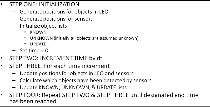
3.1 Overall Model Structure
Figure 3.1. Simulation Structure
3.2 Step One: Initialization
3.2.1 Generate Positions for Objects in Low Earth Orbit (LEO)
Before the model can determine the location of each object and sensor for a given time, the model generates a reference table for each object in the form of an array representing one complete orbit around the Earth. This array is composed of a set of XYZ coordinates
referenced by a time t. As time is incremented in the simulation, each position is determined by interpolating between the appropriate times stored in this array. This section describes the construction of this array for each object in LEO.
The positions of man-made satellites in orbit around the Earth, as well as space debris, are cataloged according to their orbital parameters. Orbital parameters are a set of six elements which can uniquely determine the position of an object with respect to the Earth. The
3.2.1.1 Converting Orbital Parameters into Time-stepped Cartesian Coordinates
There are six orbital parameters necessary to describe an object‟s position along its orbital path in space. These orbital elements describe the object of interest‟s Keplerian motion in space and are used by NASA in tracking the positions of satellites and debris in orbit. (Grimaldi, 1997). The six elements can be divided into three main groups: the elements which describe the object‟s orbital ellipse, the elements which orient this ellipse within the frame of reference, and an element which fixes the position of the object at a set time. The next section explains in detail each of the orbital elements, discussing how these elements are used within the model, and demonstrating this process through an example: the International Space Station (ISS).
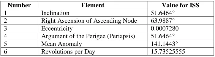
Figure 3.2. International Space Station Two-Line Elements
Figure 3.2 shows the orbital parameters for the International Space Station in the standard form of the data tracked for each known object in orbit. The shaded numbers represent the six orbital parameters, identified in Table 3.1 below.
ISS (ZARYA)
1 25544U 98067A 10060.39299677 .00014318 00000-0 10455-3 0 6766 2 25544 51.6464 63.9887 0007280 0.0341 141.1443 15.73525555646494
Table 3.1. Orbital Parameters for International Space Station
Number Element Value for ISS
1 Inclination 51.6464°
2 Right Ascension of Ascending Node 63.9887°
3 Eccentricity 0.0007280
4 Argument of the Perigee (Periapsis) 51.6464°
5 Mean Anomaly 141.1443°
6 Revolutions per Day 15.73525555
3.2.1.2 The Characteristics of the Orbit’s ellipse.
The elements which describe the characteristics of the object‟s orbital ellipse are the
eccentricity and the length of the semi-major axis. NASA uses revolutions per day instead of the length of the semi-major axis. However, the length of the semi-major axis can be derived from the revolutions per day using the equation for the Keplerian Period. (Capderou, 2005)
(3.1)
Figure 3.3. Elliptical Parameters
Then the distance from either foci to the center of the ellipse, c, can be found.
(3.2)
(3.3)
For the ISS example, these equations yield the following values: a = 3.441994, b = 3.441993 and c = 0.002506. The semi-major and semi-minor axes are very close in length, as the orbit of the ISS is nearly circular (with eccentricity 0.000728). In terms of eccentricity a perfect circle has eccentricity 0, while an eccentricity of 1 describes a parabola, and values greater than 1 describe hyperbola. For our purposes, the orbits we are interested in are ellipses, so their eccentricities lie between 0 and 1.
Assuming constant velocity around the ellipse, an X and Y coordinate system (within the plane of the ellipse) is then derived, incrementing t from 0 to 360 degrees. Equations (3.4) and (3.5) demonstrate this procedure, using Cartesian coordinates in the plane of the orbit.
c
For the remainder of equations used throughout this section, either Cartesian or Polar coordinates are used for simplicity. In the simulation, whichever set of coordinates was simpler to manipulate was used, the equations for only the sets of coordinates used within the simulation are included in this section.
(3.4)
(3.5)
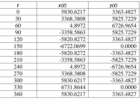
For the ISS example, incrementing t by 30 degrees, breaking the orbit into 12 steps,
following XY coordinates are obtained. The dimensions for x(t) and y(t) are with respect to the center of the Earth.
Table 3.2. XY Coordinates for ISS within Orbital Plane
t x(t) y(t)
0 5830.6217 3363.4827
30 3368.3808 5825.7229
60 4.8972 6726.9654
90 -3358.5863 5825.7229
120 -5820.8272 3363.4827
150 -6722.0699 0.0000
180 -5820.8272 -3363.4827
210 -3358.5863 -5825.7229
240 4.8972 -6726.9654
270 3368.3808 -5825.7229
300 5830.6217 -3363.4827
330 6731.8644 0.0000
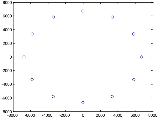
Figure 3.4. Graphical Representation of ISS Orbit within Orbital Plane
There is another orbital parameter, the Mean Anomaly, which describes the position of the object along the orbital path at a specified time. This parameter is not used due to the constant velocity assumption. The starting position of each object in orbit is determined randomly, thus eliminating the need for this parameter. In the ISS example, we would simply randomly select one of the 12 coordinate sets to start with at time 0.
3.2.1.3 The Orientation of the Orbital Plane with Respect to the Reference Plane
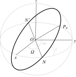
To orient the elliptical plane within the frame of reference, three angles are needed. They are the argument of the periapsis, the inclination, and the right ascension of the ascending node. These are sometimes referred to as Euler angles, or the angle of proper rotation, the angle of nutation, and the angle of precession, respectively. (Capderou, 2005)
-8000 -6000 -4000 -2000 0 2000 4000 6000 8000 -8000
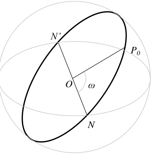
3.2.1.4 The Argument of the Periapsis
Figure 3.5. Argument of the Periapsis
In Polar coordinates, this is accomplished by the following equation. The variable θ
represents the angle (in polar coordinates), of the current position along the orbital path of the object.
(3.6)
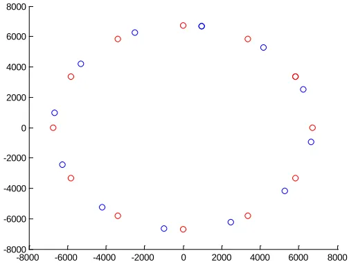
For the ISS, this rotates the XY coordinates to the following values shown in Table 3.3 and Figure 3.6. In the figure and the table, red represents the coordinates before the
transformation, and blue represents the transformed coordinates. This color coding is also followed for the remainder of the figures in this section.
N
N’
ω
P
0Table 3.3. XY Coordinates for ISS within Orbital Plane adjusted for Argument of the Perigee
t old x(t) new x(t) old y(t) new y(t)
0 5830.6217 980.3456 3363.4827 6659.4360
30 3368.3808 -2478.3861 5825.7229 6256.4078
60 4.8972 -5272.2221 6726.9654 4178.0093
90 -3358.5863 -6652.5561 5825.7229 981.1456
120 -5820.8272 -6249.5289 3363.4827 -2477.5863
150 -6722.0699 -4171.1312 0.0000 -5271.4219
180 -5820.8272 -974.2680 -3363.4827 -6651.7552
210 -3358.5863 2484.4637 -5825.7229 -6248.7270
240 4.8972 5278.2997 -6726.9654 -4170.3285
270 3368.3808 6658.6337 -5825.7229 -973.4648
300 5830.6217 6255.6065 -3363.4827 2485.2671
330 6731.8644 4177.2088 0.0000 5279.1027
360 5830.6217 980.3456 3363.4827 6659.4360
-8000 -6000 -4000 -2000 0 2000 4000 6000 8000 -8000
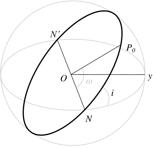
3.2.1.5 The Inclination
The inclination, i, describes the angle between the orbital plane and the equatorial plane of the Earth. In Figure 3.7, the inclination describes the angle between the orbital plane (N, O, P0) and the equatorial plane (N, O, y).
Figure 3.7. Inclination
In Cartesian coordinates, this translation is accomplished by the following equations.
(3.7)
(3.8)
(3.9)
N
N’
ω
P
0O
i
For the International Space Station, the following table and figure demonstrate this
translation, with an inclination of approximately 51 degrees, the orbit is inclined 51 degrees from the equator.
Table 3.4. XYZ Coordinates for ISS with Adjustment for Inclination
t x(t) y(t) z(t)
0 980.3456 4132.2660 5222.3046
30 -2478.3861 3882.1819 4906.2514
60 -5272.2221 2592.5087 3276.3791
90 -6652.5561 608.8135 769.4107
120 -6249.5289 -1537.3743 -1942.9138
150 -4171.1312 -3270.9854 -4133.8291
180 -974.2680 -4127.5000 -5216.2813
210 2484.4637 -3877.4158 -4900.2282
240 5278.2997 -2587.7427 -3270.3559
270 6658.6337 -604.0475 -763.3874
300 6255.6065 1542.1403 1948.9371
330 4177.2088 3275.7514 4139.8524
3.2.1.6 The Right Ascension of the Ascending Node
The last angle is the right ascension of the ascending node, Ω, which describes the angle describing the point where the orbit‟s path crosses the equatorial plane. In Figure 3.9, Ω is the angle xON, where N is the point where the path of the orbit crosses the Earth‟s equatorial plane, from below the equator to above the equator, hence „ascending,‟ O is the Earth‟s center, and x is chosen so that Ox points to a distant star to fix the reference frame.
Figure 3.9. Right Ascension of the Ascending Node
This translation is accomplished by the following equation, in cylindrical coordinates.
(3.10)
Ω
N
N’
ω
P
0O
i
y
x
Note that Equation (3.10) looks very similar to Equation (3.6), however, because of the order in which the translations are applied, they do not perform the same action. When the
argument of the periapsis was applied in Equation (3.6), it was still a two-dimensional problem within the orbital plane. In Equation (3.10) this is no longer the case, and the z coordinate is kept fixed, while orientation of the x and y coordinate‟s in the Earth‟s equatorial plane is adjusted.
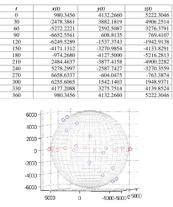
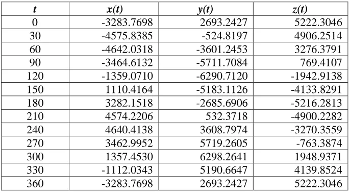
The following figure and table portray the completed orbit for the International Space Station. In its current form, the table of XYZ values is indexed by an angle t which ranges from 0 through 360 degrees. The final step for determining the reference points for the ISS is to index these XYZ coordinates by time.
Table 3.5. XYZ Coordinates for ISS with Adjustment for Right Ascension of the Ascending Node
t x(t) y(t) z(t)
0 -3283.7698 2693.2427 5222.3046
30 -4575.8385 -524.8197 4906.2514
60 -4642.0318 -3601.2453 3276.3791
90 -3464.6132 -5711.7084 769.4107
120 -1359.0710 -6290.7120 -1942.9138
150 1110.4164 -5183.1126 -4133.8291
180 3282.1518 -2685.6906 -5216.2813
210 4574.2206 532.3718 -4900.2282
240 4640.4138 3608.7974 -3270.3559
270 3462.9952 5719.2605 -763.3874
Figure 3.10. Graphical Representation of ISS Orbit with Adjustment for Right Ascension of the Ascending Node
3.2.1.7 Time
The last step is to assign a time value for each set of XYZ coordinates. This is done by multiplying the period T of the orbit by the fractional revolution of the orbit.
(3.11)
Table 3.6. XYZ Coordinates for ISS with time indexing
t (min) x(t) y(t) z(t)
0.00 -3283.7698 2693.2427 5222.3046
7.63 -4575.8385 -524.8197 4906.2514
15.25 -4642.0318 -3601.2453 3276.3791
22.88 -3464.6132 -5711.7084 769.4107
30.50 -1359.0710 -6290.7120 -1942.9138
38.13 1110.4164 -5183.1126 -4133.8291
45.76 3282.1518 -2685.6906 -5216.2813
53.38 4574.2206 532.3718 -4900.2282
61.01 4640.4138 3608.7974 -3270.3559
68.64 3462.9952 5719.2605 -763.3874
76.26 1357.4530 6298.2641 1948.9371
83.89 -1112.0343 5190.6647 4139.8524
91.51 -3283.7698 2693.2427 5222.3046
3.2.1.8 MATLAB function for Initial Object Locations
The MATLAB code for the process of defining the initial positions of each object in low Earth orbit is included in the appendix, the function name is ORBIT.
3.2.2 Generate Positions for Sensors
The initial positions for Earth-based sensors are determined through a similar method to objects in orbit. However, a simpler method for sensors can be used, since they are on the surface of the Earth. The Latitude and Longitude of the sensors position determine where the sensor orbits the Earth, as well as the sensor‟s starting position. The starting position is important, since it also fixes the sensors‟ positions relative to each other.
3.2.2.1 The Characteristic’s of the Orbit’s ellipse.
The sensor‟s rotation is modeled as an orbit along the surface of the Earth with a period of rotation of one day. The orbital plane of this orbit then becomes a circle – with eccentricity of 0. To determine the length of the semi-major axis, or radius for a circle, the Latitude is used. The Latitude measures approximately the angle between a line running from the center of the Earth to the sensor‟s location, and a line running from the center of the Earth to a point on the Equator along the same Longitude as the sensor. In reality, this number is slightly different due to the non-spherical nature of the Earth. However, for this simulation, the Earth is assumed to be spherical, therefore the Latitude is used for this simulation. To determine the radius of the circular path of the sensor, the following equation is used.
(3.12)
the semi-major and semi-minor axes are both equal to the radius, and there is only one focus, the center of the circle. In algebraic notation, a = b and c = 0. The equations then become:
(3.13)
(3.14)
3.2.2.2 The Orientation of the Orbital Plane with Respect to the Reference Plane
This orientation also simplifies for a circular orbit. Because the sensor moves in a circle parallel to the equator, the orbit never crosses the equatorial plane. Therefore, the Right Ascension of the Ascending Node is not relevant. Similarly, the inclination of this circular path to the orbital plane is 0 degrees. The only parameter that is relevant for the sensors circular orbit is the Argument of the Periapsis (or Perigee). This parameter is replaced by the Longitude of the sensor‟s position. The Longitude is similar to the Latitude in that it
3.2.2.3 Time
The last step is to assign a time value for each set of XYZ coordinates. This is done exactly the same as with objects in low Earth orbit, only using a period of 1 day. Equation (3.11) then becomes:
(3.16)
where θ represents the portion of 360 degrees represented by a given set of XYZ coordinates. The following figure and table show the results of these calculations for a sensor with
Latitude of 30 degrees.
Table 3.7. Sensor Positions with a Latitude of 30 degrees
t (min) x(t) y(t) z(t)
0.0000 2758.7239 4778.2500 3185.5000 0.0833 0.0000 5517.4478 3185.5000 0.1667 -2758.7239 4778.2500 3185.5000 0.2500 -4778.2500 2758.7239 3185.5000 0.3333 -5517.4478 0.0000 3185.5000 0.4167 -4778.2500 -2758.7239 3185.5000 0.5000 -2758.7239 -4778.2500 3185.5000 0.5833 0.0000 -5517.4478 3185.5000 0.6667 2758.7239 -4778.2500 3185.5000 0.7500 4778.2500 -2758.7239 3185.5000 0.8333 5517.4478 0.0000 3185.5000 0.9167 4778.2500 2758.7239 3185.5000 1.0000 2758.7239 4778.2500 3185.5000
3.2.2.4 MATLAB function for Initial Sensor Locations
The MATLAB code for the process of defining the initial positions of each sensor is included in the appendix, the function name is SENSORPOSITION.
3.2.3 Initialize Object Lists
the total number of objects simulated in low Earth orbit. The transitions between these lists are discussed in Section 3.4.
3.3 Step Two: Increment Time
After all positions of objects in low Earth orbit and sensors on the Earth are initialized, and the initial object lists are set, time is incremented by a set step size, dt.
3.4 Step Three: Actions at each Time Step
After the time has been incremented, the simulation performs three actions. It updates the locations of all objects and sensors in the simulation, it calculates which objects have been detected, and it updates the object lists. All of these steps are explained in detail in the following sections.
3.4.1 Update Positions for Objects in Orbit and Sensors
At each time increment in the simulation, all of the positions of the objects in orbit and the sensor locations are updated. The simulation accomplishes this task by linearly interpolating between points in the initial position locations. Because there are only a finite set of
3.4.1.1 Determining Upper and Lower Time Bounds
For a given time and a given object, the simulation must first determine how far along in time the object has moved from its initial position. The simulation divides the current time by the period of rotation of the object of interest. It then uses the remainder (or modulo) to then find the desired sets of coordinates. The simulation finds the first time index greater than this remainder. It then selects the time index below, or the last time index less than the
remainder. These two sets of coordinates are then used for interpolation.
3.4.1.2 Linearly Interpolating to Determine Current Location
Linear interpolation is used to find the desired location. Given two time referenced sets of coordinates, (x1,y1,z1,t1) and (x2,y2,z2,t2) and the current time, t, the following equations are used.
(3.17)
(3.18)
(3.19)
3.4.1.3 MATLAB function for Interpolating Object Positions
3.4.2 Calculate Detections of Objects in Orbit by Sensors
To determine which objects have been acquired by sensors in the given time period, the simulation calculates which objects have passed within the field of view of each sensor, and then determines if they have been detected based upon probability of detection.
3.4.2.1 Determining Objects within Field of View of Sensors
To determine which objects are in a given sensors field of view, the simulation calculates the angle between a line running from the center of the Earth to the sensor‟s location, and a line running from the sensor‟s location to the location of the object in low Earth orbit.
(3.20)
After determining this angle, the simulation checks to see if this angle is less than the field of view of the sensor. If it is, it moves on to the next step.
The simulation determines if the object is within the sensors field of view by calculating the azimuth and elevation from the sensor to the object in orbit. The elevation is determined from the angle θ calculated previously.
(3.21)
(3.22)
In equation (3.22) A represents the Sensor while B represents the object in LEO. This azimuth lies between -90 and 90 degrees. To convert to an azimuth between 0 and 360 degrees, the simulation determines which quadrant the resulting azimuth belongs to, adding 180 degrees if necessary.
3.4.2.2 Checking for Detection within Field of View of Sensors
If an object falls within the field of view of a sensor, the simulation generates a random number between 0 and 1 and compares the result to the probability of detection for the given sensor. The test runs for the simulation utilized both of these methods for this probability, as the actual data was unavailable. The first method was to simply set a probability of detection for an object within a sensor‟s field of view.
(3.23)
The second method was to use a probability dependent on the angle of detection, where E is the field of view of the sensor in terms of elevation, M is the midpoint angle of that field of view, and θ is the angle determined in the previous step. This method increases the
In either case, if the randomly generated number is less than the calculated probability, the object has been detected.
3.4.2.3 MATLAB function for Checking for Detections
The MATLAB code for the process of checking for detection within a sensor‟s field of view is included in the appendix, the function name is FINDANGLE. In addition, the function TESTHORIZON is also used for this process, calculating the azimuth and elevation for a given object in orbit with respect to a given sensor.
3.4.3 Update Known, Unknown, and Update Lists
There are four possible transitions between the known, unknown and update lists.
Figure 3.12. Object Lists State Diagram
If an object is detected for the first time, it moves from the unknown list to the known list. If an object is detected while it is on the update list, it moves to the known list. If an object is
UNKNOWN
KNOWN
UPDATE
λ
1λ
2λ
3detected while on the known list, it remains on the known list. As an object is detected, the last time it was detected is stored. The simulation uses this time to determine when an object moves from the Known or Update lists. If an object is on the Known list, and has not been detected in a certain amount of time, t*, the object moves to the Update lists. If an object is on the Update list, and has not been detected in a certain amount of time, s*, the object moves to the Unknown list. In this manner the lists are maintained. The rates, λi, from one object list to another, can then be determined based on the behavior of the object lists over time.
The MATLAB code for updating the object lists is included in the main program file, which is included in the appendix, the function name is SIMORBIT.
3.5 Simulation Input
The simulation uses three main sources of data. First, data for the orbital elements of the objects simulated in LEO, which are obtained by observed data. Second, data for the sensors on the surface of the Earth, which are based on the actual geographical locations and
limitations of the radars simulated. Third, various parameters within the simulation are set for each run. The following sections describe each of these inputs.
North American Aerospace Defense Command‟s (NORAD) two line format, which included approximately 5,000 objects of the 15,000 objects currently catalogued. From each of these two line elements, the six orbital parameters of interest were obtained. The entire set of 15,000 objects, or a random subset of these objects, can be used to simulate the effect of changing sensors over time. The original sets of two line elements for each object were obtained from the CelesTrak website, www.celestrak.com, associated with the Center for Space Standards and Innovation. (Kelso, 2010) Sample input data is included in the Appendices.
3.5.2 Sensor Data
For the sensors in the simulation, the locations of eight Phased Array Radar are used. These radar are part of the Space Surveillance Network utilized by the United States Department of Defense. The coordinates for each radar, as well as the azimuth and elevation limits for their fields of view are summarized in the following table, from a 2001 list furnished by Dr. Nicholas Johnson, Chief Scientist for Orbital Debris, NASA Johnson Space Center.
Table 3.8. Phased Array Radar Locations Used
Location Latitude Longitude Azimuth Limits Elevation Limits
Eglin AFB, FL 30.57° N 273.79° E 120°-240° 1°-105°
Thule AFB, Greenland 76.57° N 291.70° E 297°-177° 3°-80°
RAF Fylingdales, UK 54.37° N 359.33° E 0°-360° 4°-70°
Clear AS, AK 64.29° N 210.81° E 170°-110° 1.5°-90°
Cavalier AS, ND 48.72° N 262.10° E 298°-78° 1.9°-95°
Cape Cod AS, MA 41.75° N 289.46° E 347°-227° 3°-80°
Beale AFB, CA 39.14° N 238.65° E 126°-6° 3°-80°
The MATLAB code for loading the data for the actual sensors is located in the appendix, the function name is GETREALSENSORS.
3.5.3 Simulation Parameters
Throughout the development of the simulation, values for several key parameters were chosen. These parameters include the number of steps to partition each object‟s orbit into, the time step used to increment the simulation, the probability of detection given an object is within a sensor‟s field of view, and the time threshold for moving an object from the known list to the update list, and from the update list to the unknown list. The values chosen for these parameters are discussed in Chapter 4.
3.6 Simulation Output
Figure 3.13. Sample Simulation Output
4 EXPERIMENTATION
This section summarizes the experimentation conducted using the simulation. This includes experimentation involved in the selection of key parameters necessary for the simulation to function. In addition, this section discusses some test runs conducted to demonstrate the simulation‟s ability to model the dynamic system of sensors and orbiting objects.
0 5 10 15 20 25
0.0 0.5 1.0 1.5 2.0 2.5 3.0 3.5 4.0 4.5 5.0 5.5 6.0 6.5 7.0 7.5 8.0 8.5 9.0 9.5
N u m b e r o f O b je ct s in O rb it
Time in Days
Object Lists over Time (25 objects, 2 sensors)
Unknown
Update
4.1 Parameter Selection
4.1.1 Number of Partitions for Orbiting Objects
As mentioned previously in Chapter 3, the simulation generates a reference data set for each object in low Earth orbit. This data set consists of a time referenced set of XYZ coordinates. One important parameter for the simulation is how many time indexes, or partitions, should be used to generate this set. In the International Space Station (ISS) example illustrated previously, 12 partitions were used. This number is a little low, as the distance between each point in the data set for 12 partitions is over 3,000 kilometers.
Figure 4.1. Possible Detections by Orbit Partitions
Further runs were made varying the partitions of the sensor position while maintaining the orbit partitions constant. Figure 4.2 shows the results when orbit partitions were held
constant at 60 while the number of partitions for sensor positions was varied from 10 to 120. Again, these runs consisted of the same 100 objects and 6 sensors and ran for 1.25 days simulated time. The results of this latter experiment shows the increase in detections when the number of partitions is small. This is a result of the exaggerated field of view of the sensor when only a small number of partitions are used. For the remainder of the simulation runs referenced in this section, we used 60 partitions for both objects in orbit and sensors on the ground. 9000 9100 9200 9300 9400 9500 9600 9700 9800
0 20 40 60 80 100 120
N um be r of P os si bl e D e te ct ion s
Number of Orbit Partitions for Each Object
Figure 4.2. Possible Detections by Sensor Partitions
To determine if this size partition is appropriate, consider the resulting error in determining the position of each object in orbit by interpolation. The greater the number of partitions used, the greater the distance is between any two points, and so the interpolation between those two points will result in a greater degree of error. Using 60 partitions, the greatest magnitude of error due to interpolation would be approximately 10 km at an altitude of 1000 km above the surface of the Earth. To determine the approximate error, assume the orbit is near circular between the two points used to interpolate. In Figure 4.3, ti and ti+1 represent
8000 8500 9000 9500 10000 10500 11000 11500 12000 12500 13000
0 20 40 60 80 100 120 140
N um be r of P os si bl e D e te ct ions
Number of Position Partitions for Each Sensor
coordinates of the two points, RS, D and θ are known. The Error is then calculated using the Pythagorean Theorem. For an object in LEO with an altitude of 1000 km, this error is approximately 10.10 km.
Figure 4.3. Interpolation Error
Table 4.1 shows the resulting approximate error (in kilometers) for varying numbers of partitions for objects in orbit altitudes of 1000 km and 2000 km. For the purposes of our test runs, 60 partitions is satisfactory. If a greater level of accuracy in altitude is required, the number of partitions can be increased, with a penalty to run time.
t
iO
t
i+1θ
R
SE
R
ITable 4.1. Interpolation Error by Number of Partitions
Number of Partitions Error for an Orbit at 2000km Error for an Orbit at 1000km
10 410 361
20 103 91
30 46 40
40 26 23
50 17 15
60 11 10
70 8 7
80 6 6
90 5 4
100 4 4
4.1.2 Time Step
Figure 4.4. Effects of Changing Time Steps on Detections
The impact of this compromise is on how much time passes between each step within the simulation. The greater this time, the more likely it is that a possible detection will not be calculated, degrading the accuracy of the simulation. For a sensor with a 120 degree field of view, the diameter of what this sensor sees at 1000 km is approximately 1700 km using a simple law of cosines approximation. According to the NASA Orbital Debris Program Office, debris travels at 7 to 8 km/s. (Stansbery, 2009) This translates to roughly 420 to 480 km/min. For any time increment greater than 4 minutes, the likelihood of missing possible detections increases, as we saw in out small experiments. Again, for a desired level of accuracy, a smaller time step can be used.
0 10 20 30 40 50 60 70 80 0 10 20 30 40 50 60 70 80 90 100
2 3 4 5 6 7 8 9 10 11 12
R un Ti m e in Se conds P e rc e nt of O bj e ct s D e te ct e d
Step Size in Minutes
Effects of Changing Time Steps on Detections
Known at 12 Hours
Known at 24 Hours
4.1.3 Probability of Detection for an Object within a Radar’s Field of View
As mentioned in Chapter 3, two different methods for determining probability of detection were considered for use within the simulation. The first method involved a simple Bernoulli distribution, with a set probability of detection given the object entered the radar‟s field of view. The second method also involved a Bernoulli distribution for the probability of
detection, but also used the angle of detection to adjust this probability, as shown in Equation (4.1). The effect of this adjustment was to cause the probability of detection to increase the closer the object to be detected is to the center of the radar‟s field of view. Data sets were not available to use in validating this choice of probability, and so a value of 0.99 was selected as what is called the probability factor, which adjusts the calculated probability based on the angle of elevation. This value can be set at different levels to calibrate the model to actual probabilities if they are known.
(4.1)
where p is the probability factor, θ is the angle of elevation of the object in orbit from the
given sensor, M is the midpoint of that sensor‟s elevation range, and E is the sensor‟s
course of the simulation run. Little variation occurred as a result of this change in probability factor, as most of the probability of detection is a function of the angle of elevation.
Figure 4.5. Impact of Change in Probability Factor
4.1.4 Movement Times between Object Lists
In this simulation, an object moves between the Known List, the Update List, and the Unknown List as a function of time. This time period was set at 0.5 days, but the actual mechanism that changes objects is unknown. The value of 0.5 days was chosen by taking the average time between detections and adding two standard deviations to this value. This would allow most detections to occur within a lapse time interval. For one sensor, Eglin AFB, the average time between detections was approximately 0.1 days, or 2.4 hours. The
0 0.1 0.2 0.3 0.4 0.5 0.6 0.7 0.8 0.9 1 0 100 200 300 400 500 600 700 800 900
1 0.99 0.98 0.97 0.96 0.95 0.94 0.93 0.92 0.91 0.9
D e te ct io n R at e A ve ra ge K no w n O bj e ct s Probability Factor
Impact of Change in Probability Factor
in a value of 0.46 days for a lapse time, which was rounded to 0.5 days, or 12 hours, for simplicity. This period of time coincides with the observation that most objects are detected several times a day. (Johnson, 2004)
Figure 4.6. Simulation Results for a Lapse Time of 0.5 Days
Figure 4.6 shows the results of a simulation run with 1000 objects and 1 sensor (Eglin AFB) over a simulated time period of 10 days. Steady state behavior seems to emerge at about 1 day, or two lapse time periods. This outcome occurred in all simulated runs made during the development of the model. The steady state could not emerge prior to this time, as no object could have moved from the Known list to the Unknown list in any time less than two lapse
0 100 200 300 400 500 600 700 800 900 1000
0 1 2 3 4 5 6 7 8 9
N um be r of O bj e ct s
Simulated Time (Days)
1000 Objects, Eglin AFB Radar (0.5 L)
more, with the size of the Known list ranging from approximately 400 objects to 550 objects, a range of 150 objects. This range was approximately 50 objects with a lapse time of 0.5 days. In addition, the average value of the Known objects is approximately 450 with a lapse time of 0.25 versus an average of approximately 800 objects with a lapse time of 0.5 days. Similar results are obtained by increasing the lapse time to 0.75 hours. The longer the lapse time period, the greater chance that objects will remain in the Known list, so the average known objects increases.
Figure 4.7. Simulation Results for a Lapse Time of 0.25 Days
0 100 200 300 400 500 600 700 800 900 1000
0 1 2 3 4 5 6 7 8 9
N um be r of O bj e ct s
Simulated Time (Days)
1000 Objects, Eglin AFB Radar (0.25 L)
Figure 4.8. Simulation Results for a Lapse Time of 0.75 Days
As mentioned in the assumptions, there are other events which could potentially move an object from the Known list to the Update or even Unknown list. For a man-made satellite, these could include navigation changes triggered remotely or automatically based on certain criteria. For foreign satellites, this information would not always be known, and so satellite positions could change significantly. In addition, collisions between satellites and debris in orbit could alter the path of the satellites orbit significantly. These effects are not currently modeled within the simulation.
4.2 Test Runs
0 100 200 300 400 500 600 700 800 900 1000
0 1 2 3 4 5 6 7 8 9
N um be r of O bj e ct s
Simulated Time (Days)
1000 Objects, Eglin AFB Radar (0.75 L)
4.2.1 Demonstration of Steady State Behavior
In order for the simulation to help detect changes in performance due to the addition or subtraction of a sensor, the simulation must be able to define the state of the system at a given point in time. This state is defined by the Object Lists for a given time. The following output shows that a steady state is reached after an initial warm-up period. Because the Object Lists begin at 0 known and all unknown, objects must be detected to populate the lists. In this sample run, 5000 random objects and 5 random sensors were generated; these sensors had azimuth ranges of 0 to 360 degrees, with elevation of 0 to 90 degrees. The simulation was run for 60 days with an update rate of 2.5 days. After about 5 days in
Figure 4.9. Object Lists Over Time
4.2.2 Demonstration of Sensor Changes
The next run subtracted one sensor after 10 simulated days. Then, after 15 simulated days, the sensor was again put back into the simulation. The effect of this change can be seen in the following figure. Because the lists are not updated until the lapse time has passed, it takes two lapse time periods (or 1 days for this run), until the changes in the steady states take effect. In this example, 5000 objects in orbit and 3 sensors were used, and the model
0% 10% 20% 30% 40% 50% 60% 70% 80% 90% 100%
0 4 8 12 16 20 24 28 32 36 40 44 48 52 56
P e rc e nt of O bj e ct s
Simulated Time (Days)
Object Lists over Time
down, although the initial change in the Known lists takes less time as those objects detected are immediately moved to the Known list. There is a cyclical behavior present in the 2 sensor state, as the Eglin radar and the Thule radar remain in coverage. Once the Fylingdales radar is returned to coverage, this variation disappears and returns to the previous steady state.
Figure 4.10. Object Lists over Time with Subtraction of Sensor
4.2.3 Demonstration of Sensor Changes with Actual Data for Objects
The following figure shows the results of running the simulation with 4880 actual objects, one to three sensors (Eglin, Thule and Fylingdales) run for 30 simulated days. At the tenth day, 2 additional sensors are added (Thule and Fylingdales), and then at the fifteenth day, 1 sensor (Fylingdales), is removed.
0% 10% 20% 30% 40% 50% 60% 70% 80% 90% 100%
0 2 4 6 8 10 12 14 16 18
P e rc e nt of O bj e ct s
Simulated Time (Days)
5000 Objects, 3-2-3 Sensors
Figure 4.11. Results with Addition then Subtraction of Sensors
For each transition period, the transient time appears to take two lapse time periods, or 1 day. In Table 4.2 the numerical results of the average size of each Object List, as well as the standard deviation for each list, is displayed. The table takes these averages two days after the sensor change to avoid including the transient period in the results. The impact of the addition of two sensors can be seen in an increase from an average of 81% of objects known, to an average of 96% of objects known. In addition, the lists are less sensitive to the orbital position of the sensor. With only one sensor, there is greater variation in the size of the Known list than with three sensors. One sensor exhibits a standard deviation of 1.3% of the
0% 10% 20% 30% 40% 50% 60% 70% 80% 90% 100%
0 2 4 6 8 10 12 14 16 18 20 22 24 26 28
P e rc e nt of O bj e ct s
Simulated Time (Days)
5000 Objects, 1-3-2 Sensors
Table 4.2. Results with Addition then Subtraction of Sensors
5 FUTURE RESEARCH
Several of the assumptions used during the development of this simulation could be revisited for future improvements to this simulation. In addition, the simulation could be used as a tool in examining additional problems. Some of these assumptions include constant velocity, type of sensor utilized, and orbit perturbations. Additionally, the simulation could be useful in determining geographic locations for future and/or mobile sensors.
5.1 Constant Velocity
For this thesis, constant velocity was assumed. However, this is not the case for elliptical orbits, near circular or not. Further work could be conducted to determine the impact on the performance and accuracy of this model by using variable velocity. In addition to more accurately determining the positions of each object in LEO, this could also be used to
increase the fidelity of the detection calculations. The position and speed of the object would be used to determine whether or not an object is detected by a given radar.
Known Update Unknown 1 Sensor Mean 80.88% 11.76% 7.36% 2 to 10 Std Dev 1.31% 1.28% 0.14%
3 Sensors Mean 96.03% 0.66% 3.31% 12 to 15 Std Dev 0.17% 0.17% 0.04%
5.2 Additional Sensor Types
For this thesis, a phased-array radar was used as the basis of all sensors used. In reality, several different types of sensors, with different capabilities and reliabilities, are used as part of the Space Surveillance Network. In addition to other types of radar, some optical
telescopes, as well as the Space Fence, are key contributors to space surveillance. While optical telescopes mainly concentrate on Deep Space and Geosynchronous Orbits, they would add further fidelity to the simulation. In addition, the altitude and azimuth for each sensor could be more accurately modeled, and the resulting impact on the simulation assessed.
5.3 Orbital Perturbations
As mentioned in section 1, the non-spherical shape of the Earth has an impact on all objects in orbit around it. In addition, the gravity of the moon and other objects in space, as well as atmospheric drag, all work to perturb the orbits. Work could be done to assess the value of adding these perturbations into the simulation.
5.3.1 Orbital Perturbations due to the Non-Spherical Shape of the Earth
(5.1)
(5.2)
In Equations (5.1) and (5.2), Jn represents the harmonic coefficient for the geopotential, a quantity which is approximately 1.624 x 10⁻³ for the Earth. (Haymes, 1971), i represents the orbit‟s inclination, a the length of the orbit‟s semi-major axis, and e the orbit‟s eccentricity. For the change in the Right Ascension, Ω, the effect is that as the orbit moves around the Earth, it is pulled Westward, and so crosses the Equator (the Right Ascension), further and further from its „original‟ crossing point. The variables i and e refer to the orbit‟s inclination and eccentricity respectively. This effect is not realized for a polar orbit, with and inclination of 90 degrees, as cos(90)=0. The second element effected is the Argument of the Periapsis, ω. As the object moves around the Earth, its perigee will shift at each subsequent orbit. An
orbit around the Earth that is near equatorial (with 0 degrees inclination), will exhibit little or no change in the Argument of the Periapsis, as sin(0)=0.
For all other orbits, these changes have significant impact on the orbits. As an example, for an orbit with an inclination of 45 degrees, the Right Ascension will change by -3.37º per day, and the Argument of the Periapsis by 3.58 º per day. (Haymes, 1971)
orbit are updated throughout the run. But the values of the Right Ascension and the
Argument of the Perigee are constantly changing, so these reference tables would need to be constantly changed. One possible solution would be to generate a reference table covering the entire desired run length of the simulation. This would only have to be generated once. Then subsequent runs could interpolate positions from these pre-generated numbers that include perturbative effects.
5.4 Geographical Locations for Additional Sensors
REFERENCES
3-14, J. P. (2009, January 9). Space Operations. United States Strategic Command.
Arney, K. (2008). Global Sensor Management: Allocation of Military Surveillance Assets. Raleigh, NC: North Carolina State University.
Capderou, M. (2005). Satellites: Orbits and Missions. Paris: Springer.
Dulin, J. L. (2009). Global Sensor Management: Real-Time Reallocation of Military Assets among Competing Tasks and Functions . Raleigh, NC: North Carolina State University.
Grimaldi, B. (1997, June 19). NASA/NORAD 2-Line Elements. Retrieved February 24, 2010, from Science at NASA: http://science.nasa.gov/Realtime/rocket_sci/orbmech/state/2line.html
Haymes, R. C. (1971). Introduction to Space Science. New York: John Wiley & Sons, Inc.
Hoots, F. R., & Roehrich, R. L. (1980). Spacetrack Report No. 3. Peterson AFB, CO: Aerospace Defense Center.
Johnson, N. L. (2004). The world state of orbital debris measurements and modeling. Acta Astronautica 54 , 267-272.
Kelso, T. (2010, February 22). CelesTrak. Retrieved March 14, 2010, from CelesTrak: http://celestrak.com/
Liou, J.-C., Matney, M. J., Anz-Meador, P. D., Kessler, D., Jansen, M., & Theall, J. R. (2002). The New NASA Orbital Debris Engineering Model ORDEM2000. Houston, Texas: National Aeronautics and Space Administration.
Stansbery, E. (2009, July 22). NASA Orbital Debris Program Office. Retrieved March 13, 2010, from NASA: http://www.orbitaldebris.jsc.nasa.gov/index.html
U.S. Strategic Command Public Affairs Office. (2009, March). United States Strategic Command Fact Sheet. Retrieved March 3, 2010, from United States Strategic Command:
http://www.stratcom.mil/factsheets/snapshot/
SIMORBIT (Main Program):
function
[times,known,unknown,update,Object,Sensor,period,sensorperiod,diffTimes] = simorbit(numorbits,numsensors,userealsensors,lapsetime,usesatdata,SD,simti me)
% THESIS VERSION NOTES
% Simulates detection of objects in Low Earth Orbit (LEO) by ground based % sensors. Outputs lists of Known, Update, and Unknown sensors over time. % Either randomly generates objects and sensors, or user provided input % data. Assumes no perturbations to orbits due to shape of Earth, or other
% factors.
% DATE LAST MODIFIED: 19 March 2010
% INPUT PARAMETERS
% numorbits=1; % number of objects to simulate in orbit % numsensors=1; % number of sensors to simulate
% userealsensors; % 1 if real sensors used, 0 o/w
% lapsetime = 2.5; % time since last detection for satellite to change lists
% usesatdata = 0; % 1 if sat data used, 0 o/w generates random data % SD; % database of orbital parameters of satdata
% simtime=10; % time to be simulated (in days)
% OUTPUT
% times: vector of size n=numtimesteps with simtime at each step % known: vector of size n with values of known list at each time step % unknown: vector of size n with values of unknown list at each time step % update: vector of size n with values of update list at each time step % Object: reference table (array) of orbiting values used for run
% Sensor: reference table (array) of sensors used for run % period: vector with object periods
% sensorperiod: vector with sensor periods
% diffTimes: test vector used to calculate avg time between unique time % acquisitions
tic
% SET RUN PARAMETERS
fprintf('---START---');
% PLOT 3D REPRESENTATION OF EARTH if (graphics==1)
hold off; drawearth; end
% GENERATE ORBITS (for numorbits of objects in Low Earth Orbit) classification=zeros(1,numorbits);
LTA=zeros(1,numorbits); badorbitcount=0;
Object=zeros(4,n+1,numorbits); %1 = X, 2 = Y, 3 = Z, 4 = time period=zeros(1,numorbits);
for i=1:numorbits
if (usesatdata==1) %use external data SD e=SD(i,3); p=SD(i,4); inc=SD(i,1); L=SD(i,2); RPD=SD(i,6); M=SD(i,5);
else %use random data e=unifrnd(0.0,0.12); p=unifrnd(0,180); inc=unifrnd(0,90); L=unifrnd(0,360); RPD=unifrnd(12.5,16.5); M=unifrnd(0,360); end
[t,A,B,C,badorbit]=orbit(e,p,inc,L,RPD,M,n); %generates orbit vectors from orbital parameters
if (badorbit==1) %if orbit identified bad orbit == orbit with < 160km altitude
badorbitcount=badorbitcount+1; end
while (badorbit==1) %if badorbit detected, alter eccentricity and period until goodorbit achieved
Object(4,:,i)=t;
period(i)=1/RPD;
classification(i)=0;% 0 = unknown, 1 = known, 2 = needs updating LTA(i)=0; % Last Time Acquired
% OPTIONAL GRAPH INSTRUCTIONS % plot3(A(1),B(1),C(1),'o'); % grid on;
% axis square; % hold on;
end
badorbitcount
% TEST ORBITS FOR CRASHES
numcrash=testorbitsforcrash(Object,numorbits,n) % s/b 0!
% GENERATE SENSORS (for numsensors located on the surface of the Earth)
Sensor=zeros(4,n+1,numsensors); %1 = X, 2 = Y, 3 = Z, 4 = time sensorperiod = zeros(1,numsensors);
sensorLat = zeros(1,numsensors); sensorLong = zeros(1,numsensors); LAzimuth1 = zeros(1,numsensors); RAzimuth1 = zeros(1,numsensors); LAzimuth2 = zeros(1,numsensors); RAzimuth2 = zeros(1,numsensors); LElevation = zeros(1,numsensors); UElevation = zeros(1,numsensors); MElevation = zeros(1,numsensors);
numsensorstogenerate=numsensors+2; %to allow for adding sensors to sensor network during run
if (userealsensors==1) % Generate actual sensors
[Sensor,sensorperiod,LAzimuth1,LAzimuth2,RAzimuth1,RAzimuth2,LElevation,UE levation,MElevation]=genrealsensors(n,numsensors);
Sensor(3,:,k)=sC; Sensor(4,:,k)=st;
LAzimuth1(k) = 0.; RAzimuth1(k) = 360.;
LAzimuth2(k) = 0.; RAzimuth2(k) = 0.;
LElevation(k) = 0.; UElevation(k) = 90.;
MElevation(k) = 0.5*(UElevation(k)-LElevation(k)); sensorLat(k)=lat; sensorLong(k)=long; sensorperiod(k)=1; end end
% MAIN SIMULATION -
% - increments time by tstep for numtimeint
% - for each discrete time event, calculates position of objects in orbit % and sensors on the earth, and then determines whether or not objects % have been detected
% - updates respective lists of objects in orbit (known, update, unknown)
known=zeros(1,numtimeint); unknown=zeros(1,numtimeint); update=zeros(1,numtimeint); times=zeros(1,numtimeint); known(1)=0; unknown(1)=numorbits; update(1)=0; times(1)=tindex; printtime=160; numpossdetect=0; numdetect=0; testvector=zeros(3,numorbits); sensor1vector=zeros(3,numsensors); for j=1:numtimeint
if (j==2400) % PROGRAM subtraction of sensor numsensors=numsensors-1