Optimal Design for Parameter Estimation in EEG Problems in a 3D Multilayered Domain

(1)

Optimal Design for Parameter Estimation in EEG Problems in a

3D Multilayered Domain

March 30, 2014

H.T. Banks†, D. Rubio‡ , N. Saintier[ , M.I. Troparevsky] †_{CRSC, North Carolina State University,USA,}_{[email protected]}

‡_{Centro de Matem´}_{atica Aplicada, Universidad de San Mart´ın, Buenos Aires, ARG,}_{[email protected]} [_{Instituto de Ciencias, Universidad Nacional Gral. Sarmiento, Buenos Aires, ARG,}_{[email protected]} ]_{Dep. de Matem´}_{atica, Facultad de Ingenier´ıa, Universidad de Buenos Aires, ARG,}_{[email protected]}

Abstract

The fundamental problem of collecting data in the “best way” in order to assure statistically efficient estimation of parameters is known asOptimal Experimental Design. Many inverse problems consist in selecting best parameter values of a given mathematical model based on fits to measured data. These are usually formulated as optimization problems and the accuracy of their solutions depends not only on the chosen optimization scheme but also on the given data. We consider an electromagnetic interrogation problem, specifically one arising in an electroencephalography (EEG) problem, of finding optimal number and locations for sensors for source identification in a 3D unit sphere from data on its boundary. In this effort we compare the use of the classicalD-optimal criterion for observation points as opposed to that for a uniform observation mesh. We consider location and best number of sensors and report results based on statistical uncertainty analysis of the resulting estimated parameters.

(2)

1 Introduction

In a series of recent works [6, 7, 8, 11, 12] several authors have developed a design framework based on the Fisher Information Matrix (FIM) for a system of differential equations to determine when and where an experimenter should take samples and what variables to measure in collecting information on a physical or biological process that is modeled by a vector dynamical system. This framework has also been proposed for use in inverse problem methodologies in the context of dynamical system or mathematical model param-eter estimation when one investigates the sufficiency of the number of observations of one or more states (variables). Experimental design using the Fisher Information Matrix (FIM), which is based on sensitivity functions (traditional and generalized), is described in [7] for the case of scalar data. In [8], the authors develop an experimental design theory using the FIM to identify optimal sampling times for experiments on physical processes (modeled by an ODE system) in which scalar or vector data will be taken. The methodol-ogy can be readily applied to problems involving ordinary, partial and delay differential equations dynamics but requires both a mathematical model and astatistical model. Early efforts published in this area were concerned with parameter estimation for one dimensional dynamic systems in one space or time dimension. More recently, these ideas were successfully applied in [11] for an experimentally validated six-compartment HIV model and a thirty-eight dimensional enzyme kinetics model of the Calvin Cycle in spinach.

In [13] and [14] proof-of-concept numerical results for a distributed parameter system in a 3Done layer spherical domain are presented for several different design criteria (D-optimal, SE-optimal, IGSF-optimal). In this present effort, a more general case in 3D is studied. Motivated again by classical problems in EEG analysis, we consider a stationary process modeled by a Poisson type equation withmultiple interfacesgiven by

∇ ·(κ(x)∇u(x, θ)) = g(x, θ) x∈Ω. (1)

Hereθ∈Rpis the parameter to be estimated, Ω is the multilayered sphere inR3,κ(x) is a piecewise positive

constant conductivity function, u(x, θ)∈R, x∈∂Ω is the output and g:R3+p →Ris the source. For this

investigation we suppose that there exists a real valueθ0such that the equation (1) accurately describes the process.

For the estimation process, we formulate a statistical model [35] of the form (absolute error)

Y(x) = u(x, θ0) +E(x), x∈∂Ω, (2)

where θ0 is the vector of true values of the unknown parameters and E is a vector random process that represents observation error for the measured variables. Realizations of the statistical model (2) can be written as

y(x) = u(x, θ0) +(x), x∈∂Ω. (3)

In almost every real problem only a discrete set of output data is available. We denote{y1, ..., yn} the measurements at Λ ={x1, . . . , xn} ⊂∂Ω. In this context, the parameter valueθ0 may be estimated by an Ordinary Least Square (OLS) procedure yielding an estimate ˆθ. That is,

ˆ

θ= arg min θ∈AJΛ(θ)

whereAis the set of admisible parameter values andJΛ(θ) denotes the square errors between the measured and simulated outputs at the observation points, i.e.,

JΛ(θ) = n X

j=1

(3)

Different choices of the points x1, . . . , xn ∈Λ may lead to different estimates, and thus it is important to look for theoptimalset of observation points that will lead to an accurate parameter estimation. This is the purpose of the so-called Optimal Design methods, like D-Optimal, SE-Optimal, E-optimal design methods (see [6, 7]). For the sake of clarity, in the remainder of this article we omit the subindexes Λ onJ.

The results presented here will clearly illustrate the advantages of performing some type of design such as D-Optimal design in connection to the estimation of the parameters in the problem described by (1).

2 The EEG Inverse Problem

The electrical activity of the brain consists of currents generated by biochemical sources at the cellular level. The electric and magnetic fields that they produce can be estimated by means of Maxwell equations (see [27, 33]). Based on the properties of the tissues involved, the velocity of propagation of the electromagnetic waves caused by potential changes within the brain is such that the effect may be detected simultaneously at any point in the brain or in the surrounding tissues. This fact justifies the use of a static approximation of Maxwell equations. This approximation uncouples the equations for the magnetic and electric fields leading to a 3D Poisson-type equation with interfaces that relates the electric potential u in the head with the impressed currentC.

The equation that relates the electric potential u and the impressed currentCreads:

∇ ·(κ(x)∇u(x)) =∇ ·C, x∈Ω, ∂u

∂ν = 0 x∈∂Ω,

where the volume Ω represents the head,ν is the external normal vector andκis the conductivity function. The impressed current is often represented by an electric dipole, C(x) = q δ(x−rq), where δ is the Dirac distribution,rq is a fixed point in the brain which represents the dipole location, andqis the dipole moment [27]. Observe that, since a static approximation is considered, the values of u(x) do not depend on time; instead they correspond to a precise instant of the underlaying process.

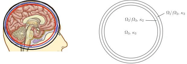
A simplified geometric model is usually considered where the head is represented by a 3D three-layered sphere. The nested subsets Ω3,Ω2\Ω3and Ω1\Ω2correspond to the brain, skull and scalp, respectively. The location of the dipole rq ∈Ω3(see Fig. 1) is in the brain. The function κ(x) represents the conductivity of

Figure 1: 3D Three-layered Domain

the tissues involved and is usually considered as a positive piecewise constant function

κ(x) =    

  

κ3 x∈Ω3, κ2 x∈Ω2\Ω3, κ1 x∈Ω1\Ω2,

(4)

Assuming that the potential and its normal derivative multiplied by the conductivity function are con-tinuous across the transition surfaces, the following interface conditions are imposed

[u] _S

i

= 0 [κ(x)∂u ∂ν]

_S

i

= 0 i= 2,3.

where [·] Si

denotes the difference between the values of the functions inside the brackets through the interface

surfaces Si=∂Ωi, i= 1, ..,3 that surround the different subsets.

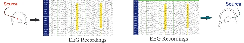
In this framework, the forward problem of EEG consists in finding the electric potential u in the head for a given current source C. Conversely the inverse problem of EEG consists in finding the location rq of the electric dipole and its moment q, for a given scalp potential u. The remaining parameters of the model κ1, κ2, κ3, as well as the radii of the spheres, are supposed to be known. We recall that the values of u(x), x∈∂Ω, do not depend on time, since they are collected at a precise instant.

Figure 2: Forward and inverse problems of EEG

Electroencephalographic source localization by noninvasive techniques is an area of interest in clinic epileptology, in particular concerning models of dipolar and distributed sources for the investigation of focal epilepsy. In this context the scalp data corresponding to an instant of a seizure should be considered. An accurate solution to the inverse problem could provide useful information to determine the location of epileptogenic zones within the brain from EEG recordings. In the last decade several authors have been working in this area. Source models were analyzed in [20, 34, 38] while forward and inverse problem solutions were studied in [28, 31, 32], among others. In [16], the authors developed a method for EEG source localization based on rational approximation techniques in the complex plane and they presented results using simulated data. We refer to the references therein for a review of the principal results concerning the inverse problem in EEG.

Since in practice the scalp potentialuis measured only at a finite set of pointsx1,· · · , xn, on the scalp where the electrodes are placed, the inverse problem of EEG consists in recoveringrq andqfrom u(x1),· · ·u(xn). Challenged by this problem, we analyze the corresponding mathematical model considering that only a finite set of potential values are available. Parameter estimation techniques and optimal design schemes are performed to solve the inverse problem accurately.

3 Mathematical model

Motivated by the above formulation we consider the following second order elliptic partial differential equa-tion (PDE)

∇ ·(κ(x)∇u(x, θ)) =∇ ·F(x, θ), in Ω, ∂u

∂ν(x, θ) = 0 in ∈∂Ω,

(5)

where Ω is the unit ball of _R3_{, and}_κ_{is a positive piecewise constant function defined by}

κ(x) =    

  

κ3 x∈Ω3, κ2 x∈Ω2\Ω3, κ1 x∈Ω1\Ω2,

0 x /∈Ω,

(6)

where Ω1= Ω and Ω2, Ω3 are balls centered at the origin with radiir2, r3 such that 0< r3< r2<1. The mathematical formulation is completely defined with the following interface and boundary conditions:

[u] _S

i

= 0 [κ(x)∂u ∂ν]

_S

i

= 0 i= 2,3. (7)

∂u(x)

∂η = 0, x∈∂G (8)

where [·]Si denotes the difference between the values of the functions inside the brackets through the surface

Si =∂Ωiandη is the external normal vector. This type of system appears in a number of applied problems such electrostatic interrogation systems, medical imaging, geophysical exploration and nondestructive testing, etc, [2, 3, 4, 5, 10, 15, 17, 18, 24, 25, 26, 29, 30].

Once again based on the formulations discussed above, we consider a functionF of the formF(x, θ) = qδ(x−rq), whereδdenotes the dirac distribution. Then the source ∇ ·F(x, θ) could represent for example an electric dipole with moment q= (q1, q2, q3)∈R3 and locationrq = (rq1, rq2, rq3)∈Ω3. The parameter of the model is thenθ= (rq, q)∈R6. Existence and uniqueness of a solution u(x, θ) to this case have been

studied in [19] and its dependence with respect to Ω and κappears in [36, 37], respectively.

In [19] the author gives an explicit formula in terms of a series, foruand its derivatives with respect to the parameters for spherical domains. This formula allows one to computeuat any point of Ω given a dipole that can be located anywhere in Ω. Since we are only interested in computing u(x) forxin the boundary ∂Ω of the domain and with a dipole located in the innermost layer, i.e., rq ∈ Ω3, we will only recall the expression ofuin this situation. The formula forugiven in [19] is

4πu(x) =q· rq krqk

(S1−S0cosω) + x

kxkS0

, (9)

where cosω= rq

krqk

x

kxk is the cosine of the angle formed by the observation pointx, the dipole locationrq and the origin, and S0,S1are given by

S0= 1 r0

X

n≥1

(2n+ 1)Rn(r0, r)Pn0(cosω), and S1= X

n≥1

(2n+ 1)R0_n(r0, r)P_n0(cosω). (10)

Here r0 =krqk,r=kxk,Pn is the n-th Legendre polynomial and Pn0 its derivative which can be computed from the recursive formula

P0(x) = 1, P1(x) =x, (11)

(n+ 1)Pn+1(x) = (2n+ 1)xPn(x)−nPn−1(x), n≥2. (12)

Finally,rq ∈Ω3 impliesr0< r3, hence the definitions ofRn andR0n given in [19] reduce to

Rn(r0, r) =−

{U3(r0,0)}12

A r

n

0, and R 0

n(r0, r) =−

{U3(r0,0)}22

κ3A r

(6)

whereA={U1(r1, r2)U2(r2, r3)U3(r3,0)}22, and the matrixUj(ra, rb) is defined as

(2n+1)Uj(ra, rb) =     

   

ra

rb

−2n−2 nr_ra

b −

ra

κj

−n(n+1)κj

rb n+ 1

!

+ n+ 1 rb

κj

n(n+1)κj

ra

nrb

ra

!

ifra, rb∈(rj+1, rj), j= 1,2

₀ 1 κ3 0 _rn

a

ifrb= 0, j= 3.

(13) We can thus rewriteRn and R0n as

Rn(r0, r) =− rn

0 (2n+ 1)κ3A

and R0_n(r0, r) =− nr

n−1 0 (2n+ 1)κ3A

, (14)

so that

S0=−1

κ3 X

n≥1

Pn0(cosω)

A r

n−1

0 and S1=− 1 κ3

X

n≥1

nPn0(cosω)

A r

n−1

0 . (15)

The formula (9) withS0 andS1 given by the previous formula (15) allow us to compute easily the solution to (5) when rq ∈Ω3 andx∈∂Ω.

4 Inverse problem formulation

We consider the inverse problem or parameter estimation for the mathematical model described by (5). It consists in estimating the unknown parameter θ= (rq, q)∈R6 from the data y1, .., yn, corresponding ton observation points atx1, .., xn on the boundary∂Ω.

We choose the Ordinary Least Square (OLS) method to calculate estimates ˆθofθ0; that is, we minimize

J(θ) = n X

j=1

|u(xj, θ)−yj|2, θ∈ A, (16)

whereA={(r, q)|r∈Ω3}. We compute the solution uof our model by means of (9). The OLS-estimator ˆθis then

ˆ

θ= arg min θ∈AJ(θ).

Theoretical results concerning existence and ill-posedness of the inverse problem associated with (5 )-(8) have been studied in [21, 22, 23].

As already noted, a statistical model is necessary to study and implement inverse problem techniques properly. Here we take the absolute error model (2) with realizations (3). In this context the inverse problem consists of the estimation of the unknown parametersθ0 from the data

yi:=u(xi, θ0) +i , i= 1, .., n,

where we assume that the additive noises1, .., nare independent realizations of a centered normal random variable with varianceσ2_.

Recall that ˆθ is a realization of a random variable ˆΘ. It can be proved that under suitable hypothesis (see [9, 35]), ˆΘ has asymptotically normal distribution

ˆ

Θ∼N(θ0,(σ2F(x1, .., xn, θ0))−1), (17)

whereF(x1, .., xn, θ)∈R6×6is the usual Fisher Information Matrix defined by

Fij(x1, .., xn, θ) = n X

k=1 ∂u ∂θi

(xk, θ) ∂u ∂θj

(7)

The partial derivatives ∂u

∂θj(xk, θ) are the traditional sensitivity functions that, assuming smoothness on u,

quantify the variations in u with respect to changes in the jth component of the parameter θ. A precise discussion of the hypothesis and the approximations involved in the above theory is given in [9].

For our model representation, the sensitivities ofuwith respect toθcan be easily computed by directly differentiating (9). The computation of the derivative ∇quofuwith respect to the momentqof the dipole is immediate from (9). For the derivative ∇rquthe author in [19] found that

4π∇rqu(x) =

rq r0

n q· rq

r0 3S₀

r0 cosω− S1

r0 +S2−2S3cosω+S4(cosω)

2₊_q_·_x_S 3−

S0

r0 −S4cosω o

+qnS1 r0

−S0

r0

cosωo+xnq·rq

r0

S3−S0

r0

−S4cosω+q·xS4o, (19)

whereS0andS1are given in (15), andS3,S4are defined as

S4= 1 r2

0 X

n≥1

(2n+ 1)Rn(r0, r)Pn00(cosω) =− 1 κ3

X

n≥1

Pn00(cosω)

A r

n−2 0 ,

S3= 1 r0

X

n≥1

(2n+ 1)R0_n(r0, r)P_n0(cosω) =− 1

κ3 X

n≥1

nP_n0(cosω)

A r

n−2 0 .

Here P_n00 is the 2nd derivative ofPn that can be calculated from (11), and one can use the expressions (14) ofRn andR0n to make the simplifications, and obtain

S2=X n≥1

(2n+ 1)Rn00(r0, r)Pn(cosω).

Then using

R00_n(r0, r) =

n(n+ 1) r2

0

Rn(r0, r)− 2 r0R

0

n(r0, r) =−

n(n−1) (2n+ 1)κ3Ar

n−2 0 ,

we find

S2=− 1 κ3

X

n≥1

n(n−1)Pn(cosω)

A r

n−2 0 .

4.1 Optimal Design

It is often useful to have some criteria to determine where samples should be taken for any type of inter-rogation problem, especially those that can be expensive and/or invasive. This is the goal of the optimal design techniques: to search for the optimal set of observation points in order to carry on the estimation procedures. Different criteria generally give rise to different selections of observation points. In most cases optimal design methods for parameter estimation problems choose the sampling distribution by minimizing a specific cost function related to the error or to the accuracy in parameter estimates. Data collected in this

optimalway will lead to parameter estimates with increased accuracy.

In view of the asymptotic distribution (17)-(18) it is natural to choose the points xi that minimize F(x1, .., xn, θ0) in some sense (see [6, 7]). A well-known and widely used optimal design method is the D-optimal criteria that consists in minimizing detF(x1, ...xn, θ)−1. Geometrically, this corresponds to min-imizing the volume of the confidence ellipsoid for the covariance matrixCov=σ2_F−1_.

With that purpose we choose the set ΛD = {x1,D. . . , xn,D} ⊂ ∂Ω of n observation points where the measurements{y1, ..., yn}are to be obtained by minimizing the function

(8)

starting with some initial set of points and consideringθ0 as an initial guess value for the parameter. After having selected the observation points, we perform OLS with the optimal set ΛD and the initial guess θ0. In the next section we present a detailed description of the way our numerical calculations were performed for the problems of interest to us in this presentation.

5 Numerical Preliminaries

Since we consider simulated data, we are able to study the actual errors and analyze the performance of Optimal Design for an optimal selection of data.

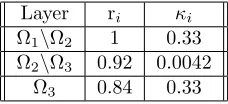
The values used in the numerical simulation are given in the following two tables. Table 1 contains the values for the mathematical model that are used in each numerical experiments. They are fixed values of the model and they are assumed to be known.

Layer ri κi Ω1\Ω2 1 0.33 Ω2\Ω3 0.92 0.0042

Ω3 0.84 0.33

Table 1: Known model values (used for all simulations).

Two different electric dipoles were chosen to illustrate a general behaviour. The first potential dipole (Example 1) is defined by F(x, y, z) = (3,4,0)δ((x, y, z)−(0.3,0.4,0))). It is a parallel dipole since its momentq= (3,4,0) is parallel to the vector positionrq = (0.3,0.4,0). The second electric dipole (Example 2) is given by F(x, y, z) = (2,−1,1)δ((x, y, z)−(0.3,0.4,0))). Note that we kept the dipole position while its moment is significantly different. These parameter values and their respective initial relative errors are shown in Table 2.

Potential Dipole (Case 1) Potential Dipole (Case 2) Positionrq Momentq Positionrq Momentq True Parameter valuesθ0 (0.3, 0.4, 0) (3, 4, 0) (0.3, 0.4, 0) (2, -1, 1) Initial Guess valuesθg (0.2, 0.2, 0.1) (2, 2, -1) (0.1, 0.2, -0.1) (0, 1, -1)

Initial Relative Error 0.4899 0.8466 0.6000 1.4142

Table 2: Parameter values for inverse problem experiments

The observation data is simulated as

yi=ui,+i, i= 1, . . . , n. (20)

where the valuesui=u(xi, θ0), i= 1,· · · , nare computed as a sum of 20 terms of the form given in (9), for θ0= (0.3,0.4,0,3,4,0) in the first example andθ0= (0.3, 0.4,0,2,−1,1) in the second.

The observation noisei at each observation point xi is calculated by the Matlab functionrandn with standard deviations σ = 0,0.05,0.1,0.15 and 0.2 to produce noise free data as well as data sets with nontrivial increasing noise levels.

(9)

0 1 2 3 4 5 6 7 0

0.5 1 1.5 2 2.5 3 3.5

φ

α

1 2 3 31

32 33 62

63

961 931

93

4

-1 -0.8 -0.6 -0.4 -0.2 0 0.2 0.4 0.6 0.8

-1 -0.5 0 0.5 1 -1 -0.8 -0.6 -0.4 -0.2 0 0.2 0.4 0.6 0.8 1

Figure 3: Rectangular grid in (φ,α) (left) and Spherical grid (right).

(αi, φj) whereαi= (i−1)∗∆α, i= 1, ...,31,φj= (j−1)∗∆φ, j= 1, ...,31. The gridpoints are numbered on the rectangular grid from left to right and from bottom to top as shown in Fig. 3 (left). The spherical gridpoints are shown in Fig. 3, on the right. Note that the bottom line of gridpoints correspond toα= 0 and the top line to α =φ. Each of these lines correspond to only one point on the unit sphere, they are (0,0,1) and (0,0,−1) in cartesian coordinates, which are thepoles. On the other hand, the extreme points of the same line are the same, due to the periodicity of trigonometrical functions. One needs to take these facts into account when considering observation points.

As mentioned before, the estimated value for the parameter is based on the initial set Λ of observation points.

We ran numerical experiments considering different numbers of measurements fromn= 7 ton= 20. For each case, the points xi, i = 1, .., nin Λ are chosen from the set of observablegridpoints as follows. First, we fix the first and the last points of Λ at the gridpoints numbered as 100 and 650, respectively; that is x1=xg100,xn =xg650. In this way we are sure that they fall far from the poles. The rest of the points are

uniformlydistributed on the numbered grid, which means

xl=xgk, k= 100 + (l−1) 550

n−1, l= 1, ..., n. (21)

6 Parameter estimation

We obtain two estimates ˆθΛ and ˆθDofθ0 performing OLS with the initial guessθg and two different sets of observations pointsx1, . . . , xn:

• the estimate ˆθΛ is obtained performing OLS with the initial guessθg and the set Λ ={x˜1, . . . ,x˜n} of observation points given by (21).

• we obtain a second estimate ˆθD of θ0 applying OLS using the observation points arising from the D-optimal design criteria as follows. We first look for a set ΛD={xD1, . . . , xDn}ofnobservation points minimizing the function

(10)

starting with Λ as initial observation points. We then perform OLS withθg as initial guess forθ and the observation points in ΛD .

The D-optimal set of observations points are calculated by means of the Matlab functionfminconwith the following optimset: MaxIter=50000,MaxFunEvals=700000,TolFun=1e-21,TolX=1e-6, with constraints 0, πforαand 0,2πforφ.

The OLS-estimate is computed by the Matlab function lsqnonlin with the same options as fmincon except that in this case we set TolFun=1e-10.

We repeat these procedures N times (generating a new set of perturbations 1, , n each time) thus we obtain 2N different estimates: N of them denoted byθj_Λ= (ˆr_qj_Λ,qˆ_Λj), j= 1, . . . , N ( OLS estimates) and the remaining ones denoted by θj_D = (ˆrj_qD,qˆj_D), j = 1, . . . , N ( D-Optimal -OLS estimates). We then compute the relatives errors forrq andq:

ej_Λ(rq) :=

krˆqj_Λ−rq0k

krq0k

, ej_Λ(q) :=kqˆ j Λ−q0k

kq0k

, j= 1, .., N,

ej_D(rq) :=

krˆqj_D−rq0k

krq0k

, ej_D(q) := kqˆ j D−q0k

kq0k , i=j, .., N,

and then average them:

¯ eΛ(rq) =

1 N

N X

j=1

ej_Λ(rq), e¯D(rq) = 1 N

N X

j=1

ej_D(rq), (22)

¯

eΛ(q) = 1 N

N X

j=1

ej_Λ(q), e¯D(q) = 1 N

N X

j=1

ej_D(q). (23)

6.1 Example 1: (parallel dipole)

We first consider a parallel dipole where the “true” values for the parameters are given by

θ0= (0.3,0.4,0,3,4,0)

and the initial “guess” values are

θg= (0.2,0.2,0.1,2,2,−1).

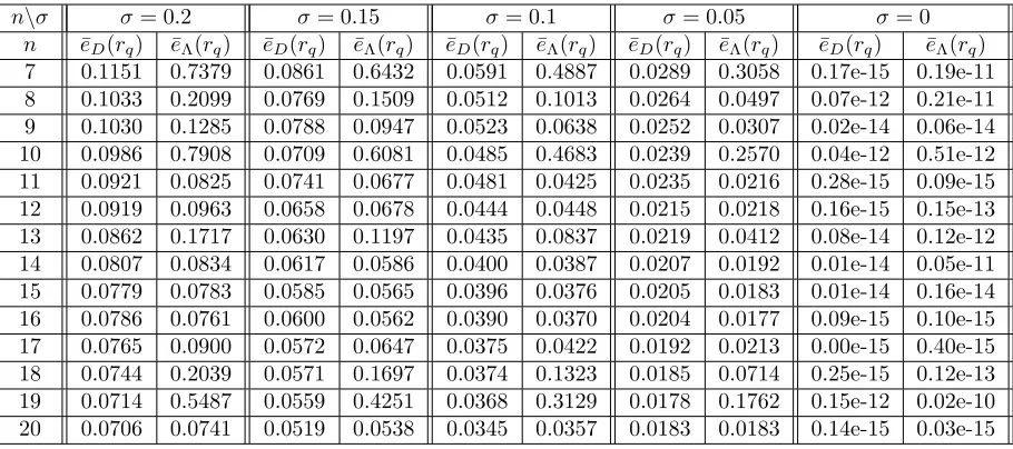
Tables 3 and 4 give the resulting values for ¯eΛ(rq), ¯eD(rq), and for ¯eΛ(q), ¯eD(q), respectively, forN = 500 with n= 7, . . . ,20 observation points and noise standard deviationsσ= 0,0.05,0.1, 0.15,0.2 for Example 1 (the parallel dipole example). These values are displayed graphically in Figures 4 (No optimal design) and 5 (D-optimal design).

We denote by ˆθΛ = ( ˆrqΛ,qˆΛ) and ˆθD = ( ˆrqD,qˆD) the average of the estimated parameters{θˆ j Λ}1≤j≤N and{θˆj_D}1≤j≤N, namely

ˆ θΛ=

1 N

N X

i=1 ˆ

θi_Λ, θˆD= 1 N

N X

i=1 ˆ θi_D.

(11)

n\σ σ= 0.2 σ= 0.15 σ= 0.1 σ= 0.05 σ= 0 n ¯eD(rq) eΛ(r¯ q) e¯D(rq) eΛ(r¯ q) e¯D(rq) eΛ(r¯ q) e¯D(rq) eΛ(r¯ q) ¯eD(rq) ¯eΛ(rq) 7 0.2855 1.1511 0.2053 1.0705 0.1299 0.8931 0.0654 0.6581 0.65e-15 0.49e-11 8 0.2079 0.6825 0.1549 0.5100 0.0995 0.3342 0.0498 0.1671 0.47e-12 0.76e-11 9 0.2024 0.4586 0.1535 0.3454 0.1017 0.2370 0.0493 0.1121 0.16e-14 0.11e-14 10 0.1990 1.2967 0.1362 1.1389 0.0931 0.9728 0.0453 0.5965 0.10e-12 0.61e-12 11 0.1946 0.3172 0.1453 0.2392 0.0958 0.1481 0.0467 0.0728 0.27e-15 0.77e-15 12 0.1790 0.3753 0.1328 0.2595 0.0845 0.1649 0.0404 0.0821 0.74e-15 0.54e-13 13 0.1837 0.3752 0.1297 0.2846 0.0896 0.1863 0.0432 0.0951 0.60e-14 0.20e-12 14 0.1636 0.3295 0.1213 0.2175 0.0793 0.1375 0.0400 0.0722 0.25e-14 0.20e-12 15 0.1601 0.2622 0.1232 0.1996 0.0793 0.1294 0.0402 0.0629 0.14e-14 0.56e-14 16 0.1521 0.2581 0.1181 0.1865 0.0744 0.1252 0.0384 0.0603 0.41e-15 0.77e-15 17 0.1546 0.2990 0.1153 0.2133 0.0732 0.1385 0.0371 0.0676 0.34e-15 0.90e-15 18 0.1489 1.0426 0.1091 0.9104 0.0727 0.7076 0.0373 0.4087 0.16e-15 0.38e-13 19 0.1481 0.8855 0.1063 0.7488 0.0720 0.6297 0.0355 0.4026 0.48e-12 0.13e-10 20 0.1360 0.2067 0.1019 0.1477 0.0695 0.1024 0.0350 0.0494 0.12e-15 0.36e-15

Table 3: Example 1. Mean relative errors ¯eD(rq) and ¯eΛ(rq) forrq as defined in (22) for different number of observation points nand different value of the noise standard deviationσ.

n\σ σ= 0.2 σ= 0.15 σ= 0.1 σ= 0.05 σ= 0

n ¯eD(rq) eΛ(r¯ q) e¯D(rq) eΛ(r¯ q) e¯D(rq) eΛ(r¯ q) e¯D(rq) eΛ(r¯ q) ¯eD(rq) ¯eΛ(rq) 7 0.1151 0.7379 0.0861 0.6432 0.0591 0.4887 0.0289 0.3058 0.17e-15 0.19e-11 8 0.1033 0.2099 0.0769 0.1509 0.0512 0.1013 0.0264 0.0497 0.07e-12 0.21e-11 9 0.1030 0.1285 0.0788 0.0947 0.0523 0.0638 0.0252 0.0307 0.02e-14 0.06e-14 10 0.0986 0.7908 0.0709 0.6081 0.0485 0.4683 0.0239 0.2570 0.04e-12 0.51e-12 11 0.0921 0.0825 0.0741 0.0677 0.0481 0.0425 0.0235 0.0216 0.28e-15 0.09e-15 12 0.0919 0.0963 0.0658 0.0678 0.0444 0.0448 0.0215 0.0218 0.16e-15 0.15e-13 13 0.0862 0.1717 0.0630 0.1197 0.0435 0.0837 0.0219 0.0412 0.08e-14 0.12e-12 14 0.0807 0.0834 0.0617 0.0586 0.0400 0.0387 0.0207 0.0192 0.01e-14 0.05e-11 15 0.0779 0.0783 0.0585 0.0565 0.0396 0.0376 0.0205 0.0183 0.01e-14 0.16e-14 16 0.0786 0.0761 0.0600 0.0562 0.0390 0.0370 0.0204 0.0177 0.09e-15 0.10e-15 17 0.0765 0.0900 0.0572 0.0647 0.0375 0.0422 0.0192 0.0213 0.00e-15 0.40e-15 18 0.0744 0.2039 0.0571 0.1697 0.0374 0.1323 0.0185 0.0714 0.25e-15 0.12e-13 19 0.0714 0.5487 0.0559 0.4251 0.0368 0.3129 0.0178 0.1762 0.15e-12 0.02e-10 20 0.0706 0.0741 0.0519 0.0538 0.0345 0.0357 0.0183 0.0183 0.14e-15 0.03e-15

Table 4: Example 1. Mean relative errors ¯eD(q) and ¯eΛ(q) for q as defined in (23) for different number of observation points nand different value of the noise standard deviationσ.

and{ui,Λ}1≤i≤ndefined in (20) using the set of observation points ΛDand Λ respectively. We then compute the estimated variances ˆσ2

Λ and ˆσ2Ddefined as

ˆ

σ2_Λ= 1 n−6

n X

i=1

ui,Λ−u(˜xi,θˆΛ) 2

, σˆ_D2 = 1 n−6

n X

i=1

ui,D−u(xDi ,θˆD) 2

(12)

The standard errorsSE(ˆθΛ), SE(ˆθD)∈R6 are then defined as

SE_k2(ˆθΛ) = ˆσ2_Λ(F(˜x1, . . . ,x˜n; ˆθΛ)−1)kk, SEk2(ˆθD) = ˆσ2D(F(x D 1, . . . , x

D

n; ˆθD)−1)kk

where k= 1, . . . ,6, and F is the Fisher matrix defined in (18). The approximate CI at the (1−α)% level for the k-th componentθ0,k ofθ0 corresponding to ˆθΛ and ˆθD are then given respectively by

[ ˆθΛ,k −t1−α/2SEk(ˆθΛ),θˆΛ,k +t1−α/2SEk(ˆθΛ) ] (24)

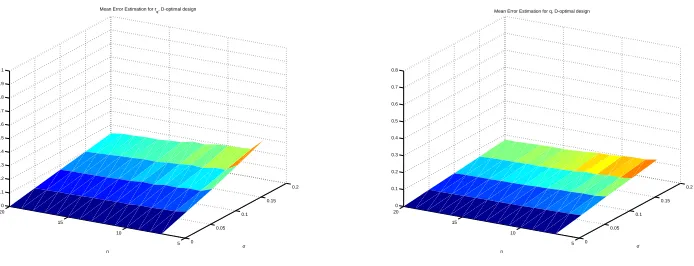
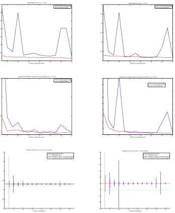
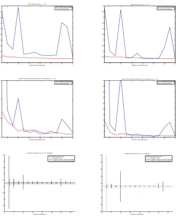
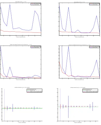
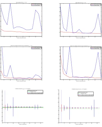
[ ˆθD,k −t1−α/2SEk(ˆθD),θˆD,k +t1−α/2SEk(ˆθD) ]. (25) The results forrq(1) (the first component ofrq) and q(1) (the first component ofq) are shown in Figures (6)-(9). Figure 6 depicts the results when σ= 0.05. From top to bottom: The mean relative errors, length of the confidence intervals (built using formula (24) (in blue) and (25)) and the confidence intervals. On the left are the results for rq(1) and on the right are the results for q(1). Similar results forσ= 0.1,0.15,0.2 are depicted in Figures 7 - 9.

0 0.05

0.1 0.15

0.2

5 10 15 20 0 0.1 0.2 0.3 0.4 0.5 0.6 0.7 0.8 0.9 1

σ

Mean Error Estimation for rq, No optimal design

n

0 0.05

0.1 0.15

0.2

5 10 15 20

0 0.1 0.2 0.3 0.4 0.5 0.6 0.7 0.8

σ

Mean Error Estimation for q, No optimal design

n

Figure 4: Mean relative errors ¯eΛ(rq) and ¯eΛ(q) (no optimal design) as functions ofnandσ.

0 0.05

0.1 0.15

0.2

5 10 15 20 0 0.1 0.2 0.3 0.4 0.5 0.6 0.7 0.8 0.9 1

σ

Mean Error Estimation for rq, D-optimal design

n

0 0.05

0.1 0.15

0.2

5 10 15 20

0 0.1 0.2 0.3 0.4 0.5 0.6 0.7 0.8

σ

Mean Error Estimation for q, D-optimal design

n

(13)

8 10 12 14 16 18 20 0

0.1 0.2 0.3 0.4 0.5 0.6 0.7

Number of observation points Mean relative error for rq - σ = 0.05

Using D-optimal design No optimal design

8 10 12 14 16 18 20

0 0.05 0.1 0.15 0.2 0.25 0.3

Number of observation points Mean relative error for q - σ = 0.05

8 10 12 14 16 18 20

0 0.5 1 1.5

Number of observation points Length of the confidence intervals for the 1st component of rq - σ = 0.05

8 10 12 14 16 18 20

0 1 2 3 4 5 6 7 8 9

Number of observation points Length of the confidence intervals for the 1st component of q - σ = 0.05

6 8 10 12 14 16 18 20

-1 -0.5 0 0.5 1 1.5 2

Number of observations Confidence Intervals for rq(1), σ = 0.05 Example 1

Real parameter value Initial guess value Confidence intervals (No optimal design) Confidence intervals (D-optimal design)

6 8 10 12 14 16 18 20

-1 0 1 2 3 4 5 6 7 8

Number of observations Confidence Intervals for q(1), σ = 0.05 Example 1

(14)

8 10 12 14 16 18 20 0

0.1 0.2 0.3 0.4 0.5 0.6 0.7 0.8 0.9 1

Number of observation points Mean relative error for r

q - σ = 0.1

8 10 12 14 16 18 20

0 0.05 0.1 0.15 0.2 0.25 0.3 0.35 0.4 0.45 0.5

8 10 12 14 16 18 20

0 0.5 1 1.5

8 10 12 14 16 18 20

0 2 4 6 8 10 12 14 16 18 20

6 8 10 12 14 16 18 20

-2 -1.5 -1 -0.5 0 0.5 1 1.5 2 2.5

6 8 10 12 14 16 18 20

-15 -10 -5 0 5 10 15 20 25

(15)

8 10 12 14 16 18 20 0

0.2 0.4 0.6 0.8 1 1.2

q - σ = 0.15

8 10 12 14 16 18 20

0 0.1 0.2 0.3 0.4 0.5 0.6 0.7

8 10 12 14 16 18 20

0 1 2 3 4 5 6 7

8 10 12 14 16 18 20

0 2 4 6 8 10 12 14 16 18 20

6 8 10 12 14 16 18 20

-3 -2 -1 0 1 2 3 4 5 6

6 8 10 12 14 16 18 20

-15 -10 -5 0 5 10 15 20 25

(16)

8 10 12 14 16 18 20 0

0.2 0.4 0.6 0.8 1 1.2

q - σ = 0.2

8 10 12 14 16 18 20

0 0.1 0.2 0.3 0.4 0.5 0.6 0.7 0.8

8 10 12 14 16 18 20

0 1 2 3 4 5 6 7 8

8 10 12 14 16 18 20

0 2 4 6 8 10 12 14 16 18 20

6 8 10 12 14 16 18 20

-3 -2 -1 0 1 2 3 4

6 8 10 12 14 16 18 20

-15 -10 -5 0 5 10 15 20 25

(17)

6.2 Example 2: (nonparallel dipole)

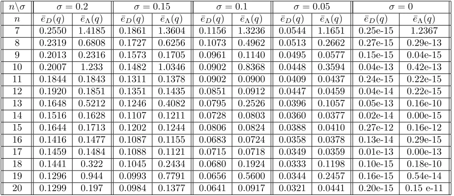
To illustrate our findings with a second example, we consider Example 2 introduced above where the moment and location arenon parallel. In this case we chose true values forθ0= (0.3,0.4,0,2,−1,1) and used initial guess parameter valuesθg = (0.1, 0.2, -0.1, 0, 1, -1). Results for different levels of noise are given in Tables 5 and 6. Findings for mean relative errors and confidence intervals of level 90 % are given in Figures 12 - 15.

n\σ σ= 0.2 σ= 0.15 σ= 0.1 σ= 0.05 σ= 0

n e¯D(rq) e¯Λ(rq) e¯D(rq) e¯Λ(rq) e¯D(rq) e¯Λ(rq) ¯eD(rq) ¯eΛ(rq) ¯eD(rq) e¯Λ(rq) 7 0.6689 1.6881 0.5211 1.6300 0.3268 1.6121 0.1615 1.4561 0.77e-015 1.8753 8 0.6009 1.2706 0.4581 1.2127 0.2975 1.0428 0.1480 0.6399 0.51e-015 0.70e-13 9 0.4500 0.6348 0.3317 0.4826 0.2133 0.3018 0.1061 0.1496 0.81e-015 0.28e-15 10 0.4272 1.5717 0.3194 1.4599 0.2005 1.2102 0.0951 0.6284 0.23e-13 0.56e-13 11 0.3774 0.5114 0.2665 0.1378 0.1790 0.2730 0.0886 0.1257 0.79e-15 0.26e-15 12 0.4544 0.4597 0.3227 0.3693 0.2077 0.2291 0.1082 0.1103 0.12e-14 0.85e-15 13 0.3573 0.9601 0.2855 0.7718 0.1748 0.5196 0.0898 0.2374 0.14e-13 0.47e-10 14 0.3666 0.4256 0.2572 0.3180 0.1653 0.2064 0.0833 0.1004 0.17e-14 0.40e-15 15 0.3891 0.4339 0.2700 0.3063 0.1865 0.2006 0.0890 0.0998 0.73e-12 0.47e-12 16 0.3235 0.4291 0.2384 0.3217 0.1589 0.2043 0.0766 0.0983 0.30e-14 0.65e-15 17 0.3107 0.4009 0.2277 0.3129 0.1559 0.1928 0.0758 0.0988 0.17e-13 0.11e-13 18 0.3306 1.079 0.2494 0.8558 0.1645 0.6944 0.0779 0.4231 0.49e-15 0.36e-10 19 0.3067 1.225 0.2317 1.0808 0.1562 0.7549 0.0783 0.3312 0.33e-15 0.34e-14 20 0.2957 0.444 0.2294 0.3061 0.1429 0.2042 0.0719 0.0976 0.14e-15 0.38e-11

Table 5: Example 2. Mean relative errors ¯eD(q) and ¯eΛ(q) for q as defined in (22) for different number of observation points nand different value of the noise standard deviationσ.

n\σ σ= 0.2 σ= 0.15 σ= 0.1 σ= 0.05 σ= 0

n e¯D(q) ¯eΛ(q) e¯D(q) ¯eΛ(q) e¯D(q) ¯eΛ(q) e¯D(q) eΛ(q)¯ ¯eD(q) eΛ(q)¯ 7 0.2550 1.4185 0.1861 1.3604 0.1156 1.3236 0.0544 1.1651 0.25e-15 1.2367 8 0.2319 0.6808 0.1727 0.6256 0.1073 0.4962 0.0513 0.2662 0.27e-15 0.29e-13 9 0.2013 0.2316 0.1573 0.1705 0.0961 0.1140 0.0495 0.0577 0.15e-15 0.04e-15 10 0.2007 1.233 0.1482 1.0346 0.0902 0.8368 0.0448 0.3594 0.04e-13 0.42e-13 11 0.1844 0.1843 0.1311 0.1378 0.0902 0.0900 0.0409 0.0437 0.24e-15 0.22e-15 12 0.1920 0.1851 0.1351 0.1435 0.0851 0.0912 0.0447 0.0459 0.04e-14 0.22e-15 13 0.1648 0.5212 0.1246 0.4082 0.0795 0.2526 0.0396 0.1057 0.05e-13 0.16e-10 14 0.1516 0.1628 0.1107 0.1211 0.0728 0.0803 0.0360 0.0377 0.02e-14 0.00e-15 15 0.1644 0.1713 0.1202 0.1244 0.0806 0.0824 0.0388 0.0410 0.27e-12 0.16e-12 16 0.1416 0.1477 0.1087 0.1155 0.0683 0.0724 0.0358 0.0378 0.13e-14 0.29e-15 17 0.1459 0.1484 0.1088 0.1121 0.0715 0.0718 0.0349 0.0359 0.01e-13 0.00e-13 18 0.1441 0.322 0.1045 0.2434 0.0680 0.1924 0.0333 0.1198 0.10e-15 0.18e-10 19 0.1296 0.944 0.0993 0.7791 0.0656 0.5600 0.0344 0.2457 0.16e-15 0.54e-14 20 0.1299 0.197 0.0984 0.1377 0.0641 0.0917 0.0321 0.0441 0.20e-15 0.15 e-11

(18)

0 0.05

0.1 0.15

0.2

5 10 15 20

0 0.2 0.4 0.6 0.8 1 1.2 1.4 1.6

σ

Mean Error Estimation for rq, No optimal design

n

0 0.05

0.1 0.15

0.2

5 10 15 20 0 0.5 1 1.5

σ

Mean Error Estimation for q, No optimal design

n

Figure 10: Mean relative errors ¯eΛ(rq) and ¯eΛ(q) (no optimal design) as functions ofnandσ.

0 0.05

0.1 0.15

0.2

5 10 15 20

0 0.2 0.4 0.6 0.8 1 1.2 1.4 1.6

σ

Mean Error Estimation for rq, D-optimal design

n

0 0.05

0.1 0.15

0.2

5 10 15 20 0 0.5 1 1.5

σ

Mean Error Estimation for q, D-optimal design

n

(19)

8 10 12 14 16 18 20 0

0.2 0.4 0.6 0.8 1 1.2 1.4

q - σ = 0.05

8 10 12 14 16 18 20

0 0.2 0.4 0.6 0.8 1 1.2 1.4

8 10 12 14 16 18 20

0 0.5 1 1.5 2 2.5 3

8 10 12 14 16 18 20

0 1 2 3 4 5 6 7 8 9 10

6 8 10 12 14 16 18 20

-0.5 0 0.5 1 1.5 2

6 8 10 12 14 16 18 20

-0.5 0 0.5 1 1.5 2 2.5 3 3.5 4

(20)

8 10 12 14 16 18 20 0

0.2 0.4 0.6 0.8 1 1.2 1.4 1.6 1.8 2

q - σ = 0.1

8 10 12 14 16 18 20

0 0.2 0.4 0.6 0.8 1 1.2 1.4 1.6 1.8 2

8 10 12 14 16 18 20

0 0.5 1 1.5 2 2.5 3

8 10 12 14 16 18 20

0 1 2 3 4 5 6 7 8 9 10

6 8 10 12 14 16 18 20

-2 -1.5 -1 -0.5 0 0.5 1 1.5 2 2.5 3

6 8 10 12 14 16 18 20

-1 0 1 2 3 4 5 6

(21)

8 10 12 14 16 18 20 0

0.2 0.4 0.6 0.8 1 1.2 1.4 1.6 1.8 2

q - σ = 0.15

8 10 12 14 16 18 20

0 0.2 0.4 0.6 0.8 1 1.2 1.4 1.6 1.8 2

8 10 12 14 16 18 20

0 0.5 1 1.5 2 2.5 3 3.5 4 4.5 5

8 10 12 14 16 18 20

0 1 2 3 4 5 6 7 8 9 10

6 8 10 12 14 16 18 20

-2 -1.5 -1 -0.5 0 0.5 1 1.5 2 2.5 3

6 8 10 12 14 16 18 20

-6 -4 -2 0 2 4 6 8 10

(22)

8 10 12 14 16 18 20 0

0.2 0.4 0.6 0.8 1 1.2 1.4 1.6 1.8 2

q - σ = 0.2

8 10 12 14 16 18 20

0 0.2 0.4 0.6 0.8 1 1.2 1.4 1.6 1.8 2

8 10 12 14 16 18 20

0 0.5 1 1.5 2 2.5 3 3.5 4 4.5 5

8 10 12 14 16 18 20

0 1 2 3 4 5 6 7 8 9 10

6 8 10 12 14 16 18 20

-4 -2 0 2 4 6 8

Number of observations Confidence Intervals for rq(1), σ = 0.2. Example 2

6 8 10 12 14 16 18 20

-10 -5 0 5 10 15 20

(23)

7 Conclusions

In this paper we have investigated a typical interrogation problem such as those used in EEG. We have shown the value of using some type of optimal design criterion (such as those studied in [6, 7, 8, 11, 12]) in determining how to best collect data. From the numerical results, we would conclude that:

• D-optimal design techniques provide a set observations points leading to a more accurate estimate of the parameters of interest. The results of this paper emphatically demonstrate the benefits of using some type of optimal design criterion (D-optimal in this case) in deciding how data should be collected in a specific application.

• For the specific EEG problem investigated, the length of the confidence intervals as well as the mean relative error do not decrease significantly for more than 10 or 11 observation points. Hence an optimal array of sensors of this size is sufficient in practice. Moreover, there are dramatic differences between estimation accuracies with a smaller number of sensors (≈7 or 8) and the optimal values of 10 or 11 sensors.

Acknowledgements

This research was supported in part by the Air Force Office of Scientific Research under grant numbers AFOSR FA9550-12-1-0188 and FA9550-10-1-0037, and in part by the National Institute of Allergy and Infectious Diseases under Grant Number NIAID R01AI071915-10.

References

[1] I. Akduman and R. Kress, Electrostatic imaging via conformal mapping, Inverse Problems18 (2002), 1659–1672.

[2] R.A. Albanese, R.L. Medina and J.W. Penn, Mathematics, medicine and microwaves,Inverse Problems, 10(1994), 995–1007.

[3] R.A. Albanese, J.W. Penn and R.L. Medina, Short-rise-time microwave pulse propagation through dis-persive biological media,J. Optical Society of America A6(1989), 1441–1446.

[4] N. D. Aparicio and M. K. Pidcock, The boundary inverse problem for the Laplace equation in two dimensions,Inverse Problems,12, (1996), 565–577.

[5] H.T. Banks, M.W. Buksas and T. Lin,Electromagnetic Material Interrogation Using Conductive Inter-faces and Acoustic Wavefronts, Frontiers in Applied Mathematics, Vol. FR21, SIAM, Philadelphia, PA, 2000.

[6] H.T. Banks, S. Dediu and S.L. Ernstberger, Sensitivity functions and their uses in inverse problems,J. Inverse and Ill-posed Problems,15(2007), 683–708.

[7] H.T. Banks, S. Dediu, S.L. Ernstberger and F. Kappel, A new optimal approach to optimal design problem,J. Inverse and Ill-posed Problems,18(2010), 25–83.

[8] H.T. Banks, K. Holm and F. Kappel, Comparison of optimal design methods in inverse problems, CRSC-TR10-11, July 2010;Inverse Problems,27(2011), 075002.

(24)

[10] H. T. Banks and F. Kojima, Boundary shape identification in two-dimensional electrostatic problems using SQUIDs, CRSC-TR98-15, April, 1998;J. Inverse and Ill-Posed Problems,8(2000), 487–504.

[11] H.T. Banks and K.L. Rehm, Experimental design for vector output systems, CRSC-TR12-11, April, 2012;Inverse Problems in Sci. and Engr.,21(2013), 1–34. DOI: 10.1080/17415977.2013.797973

[12] H.T. Banks and K.L. Rehm, Experimental design for distributed parameter vector sys-tems, CRSC-TR12-17, August, 2012; Applied Mathematics Letters, 26 (2013), 10–14; http://dx.doi.org/10.1016/j.aml.2012.08.003.

[13] H.T.Banks, D. Rubio, N. Saintier and M.I. Troparevsky, Optimal design techniques for distributed parameter systems, CRSC-TR13-01, N. C. State University, Raleigh, NC, January, 2013; Proceedings 2013 SIAM Conference on Control Theory, CT13, SIAM, (2013), 83–90.

[14] H.T.Banks, D. Rubio, N. Saintier, M.I. Troparevsky, Optimal electrode positions for the inverse problem of EEG in a simplified model in 3D, MACI,4(2013), 521–524. ISSN 2314–3282.

[15] F. Ben Hassen, Y. Boukari and H. Haddar, Inverse impedance boundary problem via the conformal mapping method: the case of small impedances,Revue ARIMA, 13(2010), 47–62.

[16] M. Clerc, J. Leblond, J-P Marmorat and T. Papadopoulo, Source localization using rational approxi-mation on plane sections,Inverse Problems, 28(2012), 1–24.

[17] D. Colton and R. Kress, Inverse Acoustic and Electromagnetic Scattering Theory, Springer Applied Mathematical Sciences, Vol. 93, 3rd ed., Springer Verlag, 2013.

[18] D. Colton, R. Kress and P. Monk, A new algorithm in electromagnetic inverse scattering theory with an application to medical imaging,Math Methods Applied Science,20(1997), 385–401.

[19] J.C. de Munck, The potential distribution in a layered anisotropic spheroidal volume conductor, J. Appl. Phys.,64 (1988), 464–470.

[20] J.C. de Munck, H. Huizenga, L.J. Waldrop, and R.M. Heethaar, Estimating stationary dipoles from MEG/EEG data contaminated with spatially and temporal correlated background noise, IEEE Trans. On Signal Processing, 50(2002), 1565–1572.

[21] A. El Badia, A inverse source problem in an anisotropic mdium by boundary measurements, Inverse Problems,16(2000), 651–663.

[22] A. El Badia, Summary of some results on an EEG inverse problem,Neurology and Clinical Neurophys-iology,2004(2004), 102.

[23] A. El Badia and M. Farah, Identification of dipole sources in an elliptic equation from boundary mea-surements: application to the inverse EEG problem,J. Inv. Ill-Posed Problems,14, (2006), 331–353.

[24] C. Gabriel, S. Gabriel and E. Corthout, The dielectric properties of biological tissues: I. Literature survey,Phys. Med. Biol. 41(1996), 2231–2249.

[25] S. Gabriel, R.W. Lau and C. Gabriel, The dielectric properties of biological tissues: II. Measurements in the frequency range 10 Hz to 20 GHz,Phys. Med. Biol.41(1996), 2251–2269.

[26] S. Gabriel, R.W. Lau and C. Gabriel, The dielectric properties of biological tissues: III. Parametric models for the dielectric spectrum of tissues,Phys. Med. Biol. 41(1996), 2271–2293.

(25)

[28] H. Huizenga, J.C. de Munck, L.J. Waldrop, and R.P. Grasman, Spatiotemporal EEG/MEG source analysis based on a parametric noise covariance model,IEEE Trans. Biomedical Engineering,49(2002), 533–539.

[29] R. Kress, Inverse Dirichlet problem and conformal mapping,Mathematics and Computers in Simulation, 2004 DOI:10.1016/j.matcom.2004.02.006

[30] R. Kress and W. Rundell, Nonlinear integral equations and the iterative solution for an inverse boundary value problem,Inverse Problems,21(2005), 1207-1223.

[31] J.C. Mosher, R.M. Leahy and P.S. Lewis, EEG and MEG: Forward solutions for inverse methods,Trans. Biomedical Engineering,46 (1999), 245–259.

[32] D. Rubio and M. I. Troparevsky, The EEG forward problem: theoretical and numerical aspects, Latin American Applied Research,36(2006), 87–92.

[33] J. Sarvas, Basic mathematical and electromagnetic concepts of the biomagnetic inverse problem,Phy. Med Biol.,32(1987), 11–22.

[34] P. H. Schimpf, C. Ramon and J. Haneisen, Dipole models for EEG and MEG,IEEE Trans. Biomedical Engineering,49(2002), 409–418.

[35] G.A.F. Seber and C.J. Wild,Nonlinear regression, Wiley Intersciences, Hoboken , NJ, 2003.

[36] M.I. Troparevsky and D. Rubio, On the weak solutions of the forward problem in EEG,J. of Applied Mathematics, 12(2003), 647–656.

[37] M.I. Troparevsky and D. Rubio, Weak solutions of the forward problem in EEG for different conductivity values,Mathematical and Computer Modeling,41(2005), 1403–1492.