DOI: 10.1534/genetics.110.115774
A Two-Stage Approximation for Analysis of Mixture
Genetic Models in Large Pedigrees
D. Habier,*
,†,1L. R. Totir
‡and R. L. Fernando
†*Institute of Animal Breeding and Husbandry, Christian-Albrechts University of Kiel, 24098 Kiel, Germany,‡Pioneer Hi-Bred International, Johnston, Iowa 50131 and†Department of Animal Science and Center for Integrated
Animal Genomics, Iowa State University, Ames, Iowa 50011 Manuscript received February 19, 2010 Accepted for publication March 30, 2010
ABSTRACT
Information from cosegregation of marker and QTL alleles, in addition to linkage disequilibrium (LD), can improve genomic selection. Variance components linear models have been proposed for this purpose, but accommodating dominance and epistasis is not straightforward with them. A full-Bayesian analysis of a mixture genetic model is favorable in this respect, but is computationally infeasible for whole-genome analyses. Thus, we propose an approximate two-step approach that neglects information from trait phenotypes in inferring ordered genotypes and segregation indicators of markers. Quantitative trait loci (QTL) fine-mapping scenarios, using high-density markers and pedigrees of five generations without genotyped females, were simulated to test this strategy against an exact full-Bayesian approach. The latter performed better in estimating QTL genotypes, but precision of QTL location and accuracy of genomic breeding values (GEBVs) did not differ for the two methods at realistically low LD. If, however, LD was higher, the exact approach resulted in a slightly higher accuracy of GEBVs. In conclusion, the two-step approach makes mixture genetic models computationally feasible for high-density markers and large pedigrees. Furthermore, markers need to be sampled only once and results can be used for the analysis of all traits. Further research is needed to evaluate the two-step approach for complex pedigrees and to analyze alternative strategies for modeling LD between QTL and markers.
D
UE to advances in molecular genetics, high-density single-nucleotide polymorphisms (SNPs) are becoming available in animal and plant breeding. These can be used for whole-genome analyses such as prediction of genomic breeding values (GEBVs) and fine mapping of quantitative trait loci (QTL). Genomic selection (GS) (Meuwissenet al. 2001) is promising to improve response to selection by exploiting linkage disequilibrium (LD) between SNPs and QTL (Hayes et al. 2009; Vanradenet al. 2009), but the accuracy of GEBVs depends on additive-genetic relationships be-tween the individuals used to estimate SNP effects and selection candidates (Habier et al. 2007, 2010). Use of cosegregation information, in addition to LD, may reduce this dependency and improve GS. Caluset al. (2008) used a variance components linear model for this purpose in which random QTL effects are modeled conditional on marker haplotypes. The covariance between founder haplotypes allows one to include LD (Meuwissen and Goddard2000), and the covariance between nonfounder haplotypes computed as in Fernandoand Grossman(1989) allows one to include cosegregation. The resulting covariance matrices,however, can be nonpositive definite, which necessi-tates bending with the effect that information can be lost (Legarra and Fernando 2009). Furthermore, accommodating dominance and epistasis is not straightforward with linear models, especially for crossbred data. In contrast with mixture genetic models, genetic covariance matrices do not enter into the analysis, and accommodating dominance and epistasis is more straightforward (Goddard 1998; Pong-Wong et al. 1998; Stricker and Fernando 1998; Du et al. 1999; Du and Hoeschele 2000; Hoeschele 2001; Yi and Xu 2002; Pe´ rez-Enciso 2003; Yiet al. 2003, 2005).
Mixture model analyses, however, are more compu-tationally demanding because the unknowns to be estimated in these analyses include the effects of un-observable QTL genotypes. In linear model analyses, in contrast, it is effects of observable marker genotypes that are estimated. The mixture model analysis can be thought of as a weighted sum of linear model analyses corresponding to each possible state for the unobserv-able QTL genotypes, where the weights are the proba-bilities of the QTL genotype states conditional on the observed marker genotypes and trait phenotypes. In practice, the analysis needs to consider all possible haplotypes at the markers also because even when all 1Corresponding author: Institute of Animal Breeding and Husbandry,
Christian-Albrechts University of Kiel, Olshausenstrasse 40, 24098 Kiel, Germany. E-mail: [email protected]
marker genotypes are observed, some of the marker haplotypes may not be known. As a result, the compu-tational burden of these analyses stems from the number of unknown genotype and haplotype states that need to be summed over being exponentially related to the number of individuals in the pedigree and the number of loci.
It can be shown that conditional on the genotypes of their parents, genotypes of offspring are independent of the genotypes of all their ancestors. This conditional independence can be exploited to efficiently compute the weighted summation in the mixture model analysis, provided the pedigree is not too complex (Lauritzen and Sheehan2003). In genetics, this strategy is called peeling (Elston and Stewart 1971; Cannings et al. 1978) and is equivalent to variable elimination in graphical models (Lauritzenand Sheehan2003). This approach, however, becomes infeasible when the ped-igree is complex and the number of loci is large. Another strategy for analysis of mixture models is based on using Markov chain Monte Carlo (MCMC) theory to draw samples of QTL genotypes and marker haplotypes conditional on the observed marker genotypes and trait phenotypes. Pe´ rez-Enciso (2003) developed an MCMC-based Bayesian analysis for a mixture genetic model that uses information from both LD and cose-gregation to fine map a single QTL, but this approach becomes computationally infeasible for whole-genome analyses without approximations.
In this article, we investigate a two-stage, approximate analysis that uses information from both LD and cosegregation. In the first stage, ordered genotypes of markers are sampled conditional only on the observed, unordered marker genotypes, ignoring information from the trait phenotypes. These samples are drawn using a Gibbs sampler with overlapping blocks (Thomas et al. 2000; Abraham et al. 2007) in which peeling is performed within a block while conditioning on varia-bles outside the block. From these samples, founder haplotype probabilities and segregation probabilities for the QTL, also called probabilities of descent of QTL (PDQs) alleles, are calculated. In the second stage, these probabilities are used to sample QTL genotypes condi-tional on the trait phenotypes. In this analysis, informa-tion from LD is incorporated by allowing the QTL allele frequencies in founders to be dependent on the marker haplotypes, and information from cosegregation is incorporated by using the PDQs from the first stage to sample QTL alleles in nonfounders. The approxima-tion comes from ignoring trait phenotypes in sampling ordered marker genotypes. A major advantage of the two-step approach is that markers have to be sampled only once and can then be used to analyze all quanti-tative traits with a mixture model.
The objective of this study is to test the hypothesis that this approximation is negligible given high-density SNPs. To test this hypothesis, results from the two-stage,
approximate analysis are compared to a full-Bayesian analysis that does not ignore the information from the trait phenotypes in sampling the ordered marker genotypes. The full-Bayesian approach was selected, because it is considered to be the ideal statistical model as it accounts for all uncertainties (Hoeschele2001). Because the full-Bayesian approach is computationally too demanding for application to GS, the approximate and full-Bayesian analyses are used to fine map within a simulated chromosomal region that is known to con-tain a QTL to make the comparison computationally feasible. If the consequences of ignoring trait pheno-types to sample ordered marker genopheno-types are negligi-ble, further research to apply mixture genetic models to GS and comparisons with linear models are justifiable.
THEORY
Statistical models: In this study, we assumed that a single additive QTL has previously been located within a given genome region and that SNP data are available for this region. The goal was to fine map this QTL into one of the genome intervals spanned by two flanking SNPs. Thus, ifKSNPs are available, there will beK1 intervals or in other wordsK1 putative QTL locations. For each putative QTL location, d, which equals the midpoint between the two flanking SNPs on an interval in cen-timorgans, a mixture genetic model can be written as
y¼1m1qda1ed; ð1Þ
whereyis the vector of trait phenotypes,mis the overall mean,qdis the column vector of unobservable genotype scores for the putative QTL locationd,ais the random additive-genetic effect of the QTL to be located, anded is the vector of residual effects for locationd. The QTL is assumed to be biallelic with allelesQ1andQ2, and thus
genotype scores in qd are set to 1, 0, and 1 for the genotypes Q1Q1, Q1Q2, and Q2Q2, respectively. The
mean phenotypic difference between the two homozy-gous genotypes is therefore 2a. Residual effects inedare modeled to be different for each putative QTL location because genotypic scores in qd depend on the QTL location for two reasons: (a) marker-QTL LD can be different for each interval and (b) the distance between true and putative QTL location affects cosegregation of marker and QTL alleles. Residual effects are assumed to be normally distributed with zero mean and variances2
ed that is specific to each QTL location.
Pr½SmðiÞ ¼Pr½Smði;1ÞY
K
j¼2
Pr½Smði;jÞ jSmði;j1Þ;
ð2Þ
where Sm(i, j) is the maternal allele state variable of individual i at locus j, the marginal probabilities, Pr[Sm(i, 1)], for allele states at marker locus 1 are written as Pr[Sm(i, 1)¼1]¼hand Pr[Sm(i, 1)¼0]¼1 – h, and lettinglx(j)¼Pr [Sm(i,j)¼1jSm(i,j– 1)¼x] for
x¼0 or 1, the conditional probabilities of allele states in (2) are written as
Pr½Smði;jÞ jSmði;j1Þ
¼
1l0ðjÞ if Smði;jÞ ¼0;Smði;j1Þ ¼0
l0ðjÞ if Smði;jÞ ¼1;Smði;j1Þ ¼0
1l1ðjÞ if Smði;jÞ ¼0;Smði;j1Þ ¼1 l1ðjÞ if Smði;jÞ ¼1;Smði;j1Þ ¼1:
8 > > > < > > > :
The map positions of markers and pedigree informa-tion are assumed known.
Unlike modeling known marker genotypes, the ge-notypic scores in qd cannot be observed. Only trait phenotypes inyand the unordered genotypes ofKSNPs denoted byMare observed. Unordered, as opposed to ordered, means that the maternal and paternal origins of the alleles are unknown.
Beta priors with shape parameters equal to 1, which reduce these distributions to a uniform distribution in the interval (0, 1), are used for both marginal and conditional probabilities of allele states. The prior for the QTL location parameterd is uniform with proba-bility 1=ðK1Þ, formit is 1, and fors2
edit is scale inverse chi square with n ¼ 4.2 d.f. and scale parameter
S2 ¼s2
eðn2Þ=n, where se2 is the simulated residual
variance in this study. The prior for a is gamma with shape parameter 0.4, which was estimated by Hayesand Goddard (2001) from published estimates of QTL effects, and the scale parameter is 1.66 such that the variance is 1 (Meuwissenet al. 2001).
Statistical methods:First, we describe general princi-ples that are common to both the full-Bayesian and the approximate, two-stage analyses. This is followed by the specific details for each approach. In Bayesian analyses, inference about model parameters such as, d; m; a; s2
ed
; h, and l are made from their posterior distributions given the observed data, which in our case consists of the unordered marker genotypes, M, and trait phenotypes, y (Sorensen and Gianola 2002). In most problems, however, computing the posterior distributions of the parameters is computa-tionally infeasible, and inferences are made by drawing samples from the joint posterior of the parameters,
pðd;m;a;s2e
d;h;ljy;MÞ; ð3Þ using MCMC techniques (Sorensenand Gianola2002). To draw samples for the variables in (3), it is often
convenient to include allele state and allele origin variables into the joint posterior. Including these variables in (3), the augmented joint posterior distribution becomes
pðd;m;a;s2
ed;h;l;Sm;Sp;Om;Opjy;MÞ; ð4Þ
where, for example,Smdenotes the maternal allele state variables andOmthe maternal allele origin variables. As an alternative to augmenting (3) with allele state and allele origin variables, it is possible to replace the maternal and paternal allele state variables in (4) by the corresponding genotype variables. Then, the aug-mented joint posterior becomes
pðd;m;a;s2e
d;h;l;G;O
m;Op;jy;MÞ; ð5Þ whereGdenotes the genotype variables. Depending on the number of alleles at a locus and the amount of missing information, sampling from one of these poste-rior distributions may be more efficient than sampling from the other. In this study, sampling from (5) was more efficient. For the purpose of describing the algorithm, however, (4) is more convenient. Thus, in the following, we use (4) to describe the sampling scheme.
After simple elimination of impossible states of allele states and origins, a Gibbs sampling strategy was used to sample the remaining variables in (4), where samples for one or more of these variables are drawn from the conditional distribution of those variables given the data and all other variables in the posterior. As de-scribed in theappendix, this joint conditional distribu-tion can be written as the product of several probability functions, each involving only a few variables. Then in principle, peeling and reverse peeling can be used to draw samples for the allele state and allele origin variables from their joint conditional distribution given all the parameters and the data (Ploughman and Boehnke 1989; Jensen et al. 1995; Heath 1997; Ferna´ ndezet al. 2001). Suppose the variables to be sam-pled by peeling and reverse peeling are denoted by
V1, . . . , Vn, where the variables are numbered in the
reverse order of peeling. Then, peeling (Elston and Stewart1971) is used to compute efficiently the mar-ginal distribution forV1, by summing over the possible
states of all the other variables. In reverse peeling (Ploughman and Boehnke 1989; Jensen et al. 1995; Heath1997; Ferna´ ndezet al. 2001), a sample forV1is drawn from this marginal distribution, and the interme-diate results from the peeling process are used to com-pute efficiently the marginal for V2 conditional on the
sampled value ofV1. Then, a sample forV2is drawn from
its marginal distribution. This process is continued for all
n variables, where at step i, intermediate results from peeling are used to compute efficiently the marginal forVi
conditional on the sampled values ofV1,V2,. . .,Vi1.
infeasible. In this case, allele state and allele origin variables can be sampled in blocks ( Jensenet al. 1995). Blocks can be formed of pedigree members and marker loci to reduce the number of variables within a block that are sampled jointly by peeling and reverse peeling conditional on the variables outside the block. Here, a pedigree block included a sire, its mates, their offspring, and the parents of the sire and the mates. Note that these blocks are overlapping, because sires and dams also occur as offspring in other blocks, a strategy also described by Thomas et al. (2000). A locus block included allele state and allele origin variables of adjacent marker loci, where a certain number of the leftmost loci of a block are also included in the previous block (except for the first block) and a certain number of the rightmost loci in the following block (except for the last block) (Abrahamet al. 2007). The overlapping of variables serves to improve mixing of the Gibbs algorithm (Abrahamet al. 2007). Allele origin and state variables of loci are peeled only within intersections of pedigree and locus blocks, while conditioning on all variables outside such an intersection. One round of sampling is completed after all intersections have been processed successively.
In this study, sampling was feasible without blocking by pedigree but using locus blocks of size eight with three overlapping loci on each side. To evaluate alternative blocking strategies, either pedigree blocking was used or the number of loci was reduced to four with two overlapping loci. To improve the estimation of PDQs, the two haplotypes of a founder are arbitrarily labeled maternal and paternal, which can be done if at least one of the observed marker genotypes of a founder is heterozygous (vanArendonket al. 1999).
The parameters inhandlare gene frequencies, and given the beta priors used for these gene frequencies, their full conditionals are also beta distributions (Sorensen and Gianola2002). The parameters for the QTL include its locationd, the mean for the traitm, the effect of the QTLa, the allele frequencies involving the QTL inl, and the residual variancese
d
2. These parameters are sampled
jointly from their full conditional using the Metropolis– Hastings algorithm, which is described in the next section. Full-Bayesian analysis: At the marker loci, as de-scribed above, peeling and reverse peeling are used to sample allele state and origin variables conditional on the current values for the allele state and allele origin variables at the QTL,h,l, and the observed, unordered genotypes at the marker loci. Thus, peeling is applied only to the marker variables in (10) with the current values of the QTL variables being treated as constants. Once all the allele state and origin variables at the marker loci were sampled, h and elements of l corresponding to markers are sampled from their full-conditional distributions, which are beta distributions that depend on the sampled allele states of the founders (Sorensen and Gianola 2002). Following this, as
described below, the Metropolis–Hastings (MH) algo-rithm is used to jointly sample a new QTL location, the parameters of this QTL, and the allele state and origin variables for the QTL at the new location, conditional on the marker allele state and origin variables.
In the MH algorithm, candidate samples are obtained by drawing from a proposal distribution, and these candidate samples are accepted or rejected according to the MH acceptance probability (Gilks and Roberts 1996). First, the location variable is sampled from an adaptive proposal, constructed from a Polya urn (Ross 2007), in which the probability of sampling locationjin roundtis given by
qtðd¼jÞ ¼
p0=ðK 1Þ1ntj p01PKk¼11ntk
; ð6Þ
where p0 is the prior degree of belief that each QTL
location is proposed with equal probability of 1=ðK1Þ, andntjis the frequency of accepted samples in locationj, with n0j ¼ 0. Given the proposed QTL location, the
proposed value formis drawn from a normal distribu-tion, forafrom gamma, fors2
ed from a scaled inverse chi square, and for allele frequencies from beta distributions, where the parameters of these distributions are chosen such that the proposed values are in the neighborhood of the most recently accepted values for the proposed QTL location as described in theappendix.
Given the proposed location and QTL parameters, the QTL allele state and origin variables are sampled from the full-conditional distribution for these variables. Peeling and reverse peeling are used to sample these variables jointly conditional on the allele state and origin variables at the markers and all the relevant parameters. Here, peeling is applied only to the QTL variables in (10) with the current values of the marker variables being treated as constants. Finally, the proposed QTL location, QTL parameters, and QTL origin and state variables are accepted or rejected according to the MH algorithm in which the probability of acceptance is
aðud;ud9Þ ¼min 1;
pðyjud9Þpðud9jMÞqðudjy;MÞ pðyjudÞpðudjMÞqðud9jy;MÞ
;
whereud is the vector of the currently accepted values for the variables being sampled,ud9 is the vector of the
proposed values for these variables, pðyjudÞ and pðyjud9Þ denote distributions for the data models, pðudjMÞ and pðud9jMÞ are prior distributions, and qðudjy;MÞandqðud9jy;MÞare proposal distributions.
sample all the variables within a block, except that the joint distribution (Equation A1 in the appendix) is constructed without any QTL related probabilities. These samples are then used to estimate two types of probabilities. The first type consists of the joint proba-bilities of the maternal (Pr[hm(i,d)jM]) and paternal (Pr[hp(i,d)jM]) marker haplotypes, consisting of the allele states of the two markers flanking each of theK– 1 potential QTL positions in the founders. They are estimated from the sampled allele state variables in the founders. The second type consists of the joint probabilities of the allele origin variables for the ma-ternal and pama-ternal marker haplotypes, Pr[Om(i,d– 1),
Om(i,d11)jM] and Pr[Op(i,d– 1),Op(i,d11)jM], flanking each of theK– 1 potential QTL positions in nonfounders. They are estimated from the sampled allele origin variables of nonfounders. With the allele origin variable for a given marker allele being either 0 or 1, there are four possible combinations of allele origin variables for a two-marker haplotype. Given one of these combinations, the conditional PDQ can be calculated for the maternal and the paternal QTL allele of a nonfounder at the midpoint of the flanking markers using formulas shown in Table 1, assuming no interfer-ence. The PDQs conditional on the observed, unor-dered marker genotypes, Pr[Ox(i,d)jM], are derived by weighting the conditional PDQ for each combination of segregation indicators of a two-marker haplotype with their corresponding probabilities,i.e., Pr[Om(i,d – 1),
Om(i,d11)jM] and Pr[Op(i,d– 1),Op(i,d11)jM]. The parameters of the mixture model in the two-stage approximate method ared,m,a, andse
d
2as in the
full-Bayesian analysis, with a new parameter p for the conditional allele frequency at the QTL given the allele states at the flanking markers. The vector pd¼
½pd;00;pd;01;pd;10;pd;11has four elements, where
pd;lm ¼Pr½Sxði;dÞ ¼1jhxði;dÞ ¼ ðl;mÞ; ð7Þ
forx¼morp, and (l,m)¼(0, 0), (0, 1), (1, 0), or (1, 1). As in the full-Bayesian analysis, these parameters, the allele states, and the allele origin variables at the QTL are sampled jointly using the MH algorithm in the
second stage of the approximate method. However, while Equation A1 in theappendixwas used in the full-Bayesian analysis to sample QTL allele states and allele origin variables conditional on the allele states and allele origin variables at the flanking markers, here QTL variables are sampled conditional on the observed, unordered marker genotypes,M, as described below.
The joint distribution for QTL allele state and allele origin variables given the observed, unordered marker genotypes and the QTL parameters is expressed as
pðSm
d;S
p
d;Omd;O
p
djm;s2e;pd;MÞ
} Y
i;j
Pr½yijjSmði;dÞ;Spði;dÞ
Y
i#F
Pr½Smði;dÞ jMPr½Spði;dÞ jM Y
i.F
Pr½Smði;dÞ jSmðdi;dÞ;Spðdi;dÞ;Omði;dÞPr½Omði;dÞ jM
3Pr½Spði;dÞ jSmðs
i;dÞ;Spðsi;dÞ; Opði;dÞPr½Opði;dÞ jM; 8
> > > > > > > > > < > > > > > > > > > :
ð8Þ
where Fis the number of founders,sidenotes the sire and di the dam of individuali, and Pr[Sx(i,d) jM] is computed as
Pr½Sxði;dÞ jM ¼X
lm
pd;lmPr½hix;d¼ ðl;mÞ jM: ð9Þ
Peeling and reverse peeling are used to draw candidate samples for the QTL allele states and allele origin vari-ables from (8), and candidate samples for the parameters were drawn in the neighborhood of their current values as described in the full-Bayesian analysis. These samples were accepted or rejected using the MH rule.
Sample scheme:Each MCMC round has two types of sampling steps to update QTL parameters and variables. These were calledjumpandresamplesteps, where each of these two steps can be performed a different number of times within each MCMC round. In thejumpstep, a new QTL location other than the one currently accepted is proposed along with its parameters and variables, whereas in the resample step, new parameters and variables of the QTL location currently accepted are proposed. The jumpstep was performed 30 times and theresamplestep 20 times in each round.
TABLE 1
Conditional probabilities of descent,pmm¼Pr[Sm(i,d)*Sm(d
i,d)jOm(i,d– 1),Om(i,d11)] andpmp¼Pr[Sm(i, d)*Sp(d
i,d)jOm(i,d– 1),Om(i,d11)], of the maternal allele of individualiat QTL positiond,Sm(i,d),
from the maternal and paternal allele of its motherdi,Sm(di,d) andSp(di,d), depending on the
segregation indicators at the flanking SNPs,Om(i,d– 1) andOm(i,d11)
Om(i,d– 1) Om(i,d11) pmm pmp
0 0 (1 –r1)(1 –r2)/(1 –r12) r1r2/(1 –r12)
0 1 (1 –r1)r2/r12 r1(1 –r2)/r12
1 0 r1(1 –r2)/r12 (1 –r1)r2/r12
1 1 r1r2/(1 –r12) (1 –r1)(1 –r2)/(1 –r12)
The full-Bayesian approach was run for 24 hr and each step of the two-step approach for 12 hr, where the burn-in was always 5000 rounds. The processor used for all computations was an AMD Opteron 2352 with 2.1 GHz and 4 Gb memory.
SIMULATIONS
Simulations were used to study the consequences of neglecting the information that trait phenotypes pro-vide to infer allele states and origins of markers and of using alternative blocking strategies for the Gibbs sampler on estimation of QTL parameters and on prediction of GEBVs. The aim was (1) to simulate marker–QTL LD similar to that found recently in real cattle populations, where the study of de Roos et al. (2008) served as a template, and (2) to simulate marker–QTL LD that is higher than in the first scenario to compare the full-Bayesian with the two-step approach at low and high LD. The two scenarios differed only in the effective size of the simulated base populations, which were randomly mated, including selfing, for 1000 discrete generations. Effective sizes of the two base populations were 1500 and 500 individuals in scenarios 1 and 2, respectively. The population was reduced to a size of 100 individuals after 1000 generations and randomly mated for another 15 generations. The population was then gradually increased over the next 10 generations to obtain a population of 800 males and 800 females in generation 1025. In the following 3 generations, 80 sires were randomly selected and mated to 800 dams in each discrete generation. Each female had one male and one female offspring and thus each sire had 10 sons and 10 daughters. Individuals of generation 1028 were considered as founders of the pedigree used for fine mapping. Four additional gen-erations were generated by selecting 20 sires from the male offspring in each generation at random and mating them to 200 founder dams from generation 1028, where different founder dams were used in each generation. Each mating produced one male offspring and thus each sire had 10 offspring. It was assumed that neither phenotypic nor marker data were available for dams and thus they were not included in the analyses. In total, the pedigree consisted of 820 individuals, the 20 founder sires and 200 male offspring in each of the 4 subsequent generations. Because dams were not in-cluded in the analyses, the pedigree had no loops and thus QTL variables could be peeled without pedigree blocking. Otherwise further approximation strategies were needed, which must be different from those used for SNPs. This is discussed in thediscussion.
A single-chromosome segment of length 5 cM was simulated with 2000 evenly spaced SNPs in generation 1. A total of 300 QTL were randomly distributed among those SNPs and their effects were sampled from a
gamma distribution with shape 0.4 and scale 1.66 as used by Meuwissenet al. (2001). All loci were simulated to be biallelic with initial allele frequencies 0.5 and in Hardy–Weinberg and linkage equilibrium. The muta-tion rate for both SNPs and QTL was 2.53105, which is larger than estimates of actual mutation rate to ensure that enough loci are segregating for statistical analyses after 1025 generations of random mating. However, it can be shown that the mutation rate has only a small effect on LD in this simulation. Recombinations were modeled according to a binomial map function, where the maximum number of uniformly and independently distributed crossovers on a chromosome of 1 M was four (Karlin 1984),i.e., assuming interference. In genera-tion 1028 (founder generagenera-tion of the pedigree), the chromosome was first divided into 100 bins with an equal number of SNPs in each bin. Then, within each bin the SNP with highest minor allele frequency was selected. Next, the QTL with frequency closest to 0.5 was selected as the only locus with effect on the quantitative trait. Twenty adjacent SNPs around this QTL were finally selected for fine mapping, where the position of the QTL was random between SNPs 4 and 16. Because each of the 100 bins had a length of 0.05 cM, the expected length of the fine-mapping region was 1 cM.
Heritability (h2) of the quantitative trait was set to 0.05 by rescaling the QTL effect in generation 1028. Pheno-types were calculated as the sum of the QTL genotype effect of an individual and a residual effect sampled from a standard normal distribution. To compare methods also at a higherh2of 0.3, residual effects were resampled with a residual variance of 0.123. The 820 individuals were all phenotyped for the quantitative trait and genotyped for the 20 SNPs.
Comparison of methods: For both the full-Bayesian approach and the two-step approach, the mean absolute difference between estimated and true value ofdanda
was obtained as
mean absolute difference ¼
P
j jˆzjzjj
n ;
whereˆzjandzjdenote, respectively, posterior mean and true value of replicatejof the simulation, andnis the number of replicates. The posterior mean of the genotypic score of an individuali,ˆqi, was derived from samples of allele states at all putative QTL locations. The mean absolute differences between true and estimated genotypic scores were first averaged over individuals and then over replicates. The ability to estimate LD between the QTL and two-SNP intervals was evaluated with regression R2 (Zhao et al. 2005), which was calculated for each putative QTL location in each iteration of the MCMC algorithm as
Rd2¼
P
where Pr[hx(i,d)]¼Pr[Sx(i,d– 1),Sx(i,d11)] (x¼m or p) denotes the frequency of the maternal or paternal two-SNP haplotype at QTL location d, and Pr[Sx
(i, d)jhx
(i, d)] describes LD between the QTL and the flanking SNPs at locationd. This conditional probability is obtained fromhand elements inlin the full-Bayesian approach, whereaspdis used in the two-step approach. The true R2
d was determined using true frequencies from the simulation. Because LD is different for every putative QTL location, the absolute difference between true R2
d and posterior means was calculated for each location separately, weighted by the posterior probabil-ities ford, and summed to obtain a single value. These values were finally averaged over replicates. The GEBV of an individualiwas calculated asAiˆ ¼ˆqiaˆ, whereaˆis the posterior mean of the QTL effect. The accuracy of GEBVs was calculated as the correlation between true simulated breeding values and GEBVs. Finally, the number of MCMC rounds obtained for sampling SNPs and QTL variables was recorded. Paired t-tests were applied to test for significant differences between com-parison criteria of the full-Bayesian and two-step ap-proach when replicates were simulated with the same LD, whereas normalt-tests were used across LD scenarios.
RESULTS
The average length of the genome regions obtained from 32 replicates of the simulation was 0.94 (60.005) cM containing 20 SNPs at intervals of 0.05 (60.001) cM and with minor allele frequency of 0.46 (60.01). The mean fraction of ordered SNP genotypes and paternal segregation indicators that could be determined by simple genotype elimination prior to sampling was 24.8% each. Average allele frequency of the QTL was 0.5 (63 3 104) such that the mean simulated QTL effect was 0.324 (613106). The extent of LD between pairs of QTL and SNPs generated after 1028
genera-tions along with that reported recently for real cattle populations (deRooset al. 2008) is depicted for a map distance of up to 1 cM in Figure 1. Averager2decreased exponentially with increasing distance and was similar for all populations above a distance of 0.6 cM. As expected, average r2 at shorter distances was substan-tially higher for 500 effective individuals (Ne) than for
1500, and values forNe¼1500 matched well with those
for real cattle populations, although they were lower at distances ,0.01 cM. Average r2 at 0.025 cM, which corresponds to the average distance between a putative QTL location and a flanking SNP, was 0.5 forNe¼500
and 0.24 for Ne ¼ 1500. Figure 2 presents true r2
between the QTL and SNPs used for mapping as well as trueR2between the QTL and each two-SNP interval for selected replicates of the simulation withNe¼1500.
The latter LD measure, which was the relevant one in this study because two-SNP haplotypes were used to model LD, was often substantially .r2for each of the flanking SNPs, especially when r2 was incomplete. In replicates 1, 4, 5, and 6, R2 clearly decreased with increasing distances to the true QTL position, whereas in replicates 2 and 3 the difference between close and distant putative QTL locations was not as distinct, where a clearR2peak was missing in replicate 2. Further, note that the SNP interval with the highestR2may not be the one closest to the true QTL position, as can be seen in replicates 2–4.
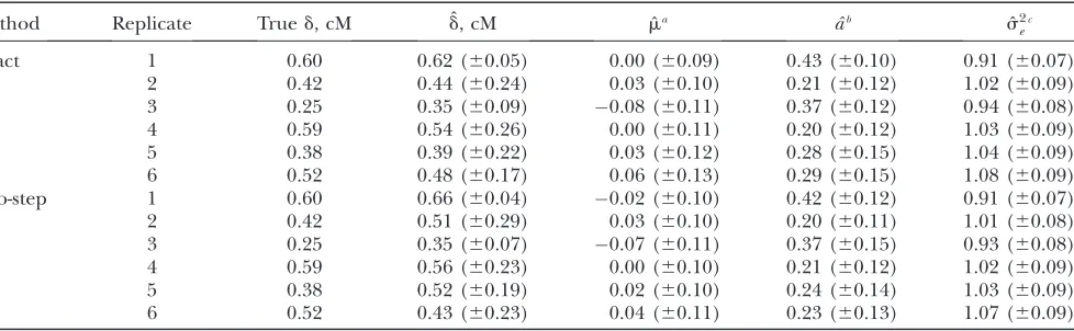
Figure 2 also presents posterior distributions of the QTL location parameter d for the exact and two-step approaches. Except for replicate 2, which had low and almost uniform distributed R2, the positions of poste-rior modes agreed with locations of the highest R2 values in both methods. For replicates with high R2, the posterior distributions were generally highly peaked and standard deviations of the QTL location were small, as can be seen for replicates 1 and 3 in Table 2. Posterior distributions of both methods matched well for these Figure 1.—Average linkage
disequi-librium between pairs of QTL and SNPs measured asr2against map distance in centimorgans (cM) obtained from sim-ulations using 500 and 1500 effective in-dividuals (Ne) in the base population and taken from the study of DeRoos
two replicates, but in 5 and 6, which also had highR2, they differed apparently and standard deviations were high (Figure 2 and Table 2). With low R2, posterior modes were less distinct and standard deviations were usually larger than with highR2(replicates 2 and 4). An explanation for the shape of the posterior distributions can be found in the estimatedR2depicted in Figure 3. In general, estimatedR2agreed well between both meth-ods, but it was much lower than the true R2. Clear maxima resulted only for replicates 1 and 3, whereas estimated R2 was almost flat around the true QTL
position in replicates 5 and 6, although there were two-SNP intervals with high trueR2. Thus both methods had difficulties in these replicates to distinguish be-tween putative QTL locations surrounding the true QTL position, resulting in different posterior distribu-tions. For lowR2, the estimatedR2was usually flat as in replicates 2 and 4.
Estimates and standard deviations of m, a, and s2 e
obtained with both methods were very similar (Table 2). Replicates 1 and 3 were conspicuous compared to the other selected replicates in thatawas overestimated and Figure2.—True QTL location (vertical dashed line), simulated linkage disequilibrium between the QTL and SNPs used for
s2
e underestimated, which was generally the case
when trueR2was high and estimated sufficiently well. Otherwise a tended to be underestimated and s2 e
overestimated.
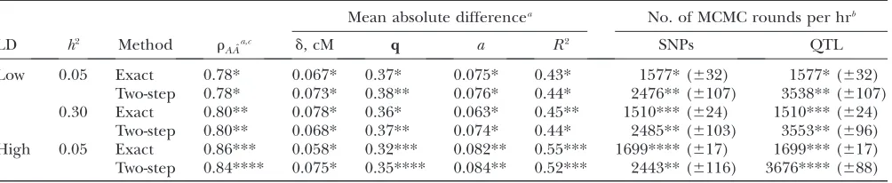
Table 3 shows accuracies of GEBVs and mean absolute differences (MAD) between true and estimated values ofd,q,a, andR2, as well as the average number of MCMC rounds per hour obtained for sampling SNP and QTL variables for the exact and two-step approaches, de-pending on the extent of LD andh2. In all scenarios, and especially at high LD, the MAD of q was significantly lower for the exact approach than for the two-step approach. The accuracy of GEBVs of the exact ap-proach, however, was only higher at high LD, whereas both methods had equal accuracies at low LD. The MAD ofd,a, andR2showed no clear differences with respect to both h2 and the method used. With high LD, accuracies of GEBVs as well as MAD of aand R2were higher compared to low LD, whereas MAD of q was significantly lower. The MAD ofdranged between 0.058 and 0.078 cM, which means that the distance between estimated and true QTL position was on average 6–8% of the size of the genome region prior to fine mapping. Similarly, MAD ofqwas 16–18% of the initial range of 2, and MAD ofawas 19–26% of the simulated QTL effect. Average number of MCMC rounds per hour for sampling both SNP and QTL variables was always higher for the two-step approach (Table 3). Because the exact approach was run for 24 hr and each step of the two-step approach for 12 hr, the total number of rounds for SNPs was higher for the exact approach, but lower for QTL variables. Furthermore, the number of rounds in the exact approach was lower with higherh2, but higher at high LD. As expected for the two-step approach, the number of rounds was not different for sampling SNPs
regarding h2 and LD, but the number of rounds was higher for sampling QTL variables at high LD as in the exact approach. The reason is that more QTL locations were in high LD with the QTL than in the low-LD scenario, and thus it was easier for the MCMC chain to jump between QTL locations, thereby reducing the average number of iterations used in thejumpstep such that the next MCMC round could start more rapidly.
Results of using alternative strategies for sampling SNP variables in the two-step approach are shown in Table 4. Pedigree blocking (alternative a) had no effect on both accuracy of GEBVs and mean absolute differ-ences, but the number of MCMC rounds for sampling SNP variables was higher (compare with Table 3, low LD,
h2¼0.05, two-step approach). If, however, the size of the locus blocks was reduced from eight to four and the number of overlapping loci from three to two (alterna-tive b), MAD of q was higher and accuracy of GEBVs significantly lower. Increasing the block size above eight loci did not improve precision of QTL parameter estimates or GEBVs (results not shown).
DISCUSSION
The primary goal of this study was to utilize in-formation from LD and cosegregation for whole-genome analyses with a mixture genetic model, because accommodating dominance, epistasis, and imprinting is straightforward with such a model. To make it compu-tationally feasible for a large number of high-density markers and large pedigrees, an approximate strategy was proposed in which (1) marker and QTL variables are not sampled jointly as in an exact approach, but in two consecutive steps, and (2) a Gibbs sampler with overlapping blocks is used to sample marker variables.
TABLE 2
True QTL location in centimorgans (cM) as well as posterior means and standard deviations ofd,m,a, ands2
e obtained
by the exact and two-step approaches for selected replicates of the simulation with 1500 effective individuals in the base population and a heritability of 0.05
Method Replicate Trued, cM dˆ, cM mˆa aˆb sˆ2
ec
Exact 1 0.60 0.62 (60.05) 0.00 (60.09) 0.43 (60.10) 0.91 (60.07)
2 0.42 0.44 (60.24) 0.03 (60.10) 0.21 (60.12) 1.02 (60.09)
3 0.25 0.35 (60.09) 0.08 (60.11) 0.37 (60.12) 0.94 (60.08)
4 0.59 0.54 (60.26) 0.00 (60.11) 0.20 (60.12) 1.03 (60.09)
5 0.38 0.39 (60.22) 0.03 (60.12) 0.28 (60.15) 1.04 (60.09)
6 0.52 0.48 (60.17) 0.06 (60.13) 0.29 (60.15) 1.08 (60.09)
Two-step 1 0.60 0.66 (60.04) 0.02 (60.10) 0.42 (60.12) 0.91 (60.07)
2 0.42 0.51 (60.29) 0.03 (60.10) 0.20 (60.11) 1.01 (60.08)
3 0.25 0.35 (60.07) 0.07 (60.11) 0.37 (60.15) 0.93 (60.08)
4 0.59 0.56 (60.23) 0.00 (60.10) 0.21 (60.12) 1.02 (60.09)
5 0.38 0.52 (60.19) 0.02 (60.10) 0.24 (60.14) 1.03 (60.09)
6 0.52 0.43 (60.23) 0.04 (60.11) 0.23 (60.13) 1.07 (60.09)
a m¼0. b
a¼0.324. c
s2
Simple pedigrees without females and fine-mapping scenarios with realistic LD were simulated to compare the exact with the two-step approach. Estimates for QTL location, additive effect of QTL, and LD parameters obtained by both methods were very similar. When LD between the QTL and two-SNP intervals could not be estimated sufficiently well to distinguish between puta-tive QTL locations, posterior distributions of the QTL location parameter slightly differed between methods. Although the exact approach always performed better in estimating QTL genotypes, accuracy of GEBVs was
identical for the two methods at realistically low LD. If, however, LD was higher, the exact approach resulted in a slightly higher accuracy of GEBVs. Pedigree blocking used to sample SNP variables had neither an effect on estimates of QTL parameters nor one on accuracy of GEBVs, whereas a smaller locus block size reduced the accuracy of GEBVs.
Modeling of LD and cosegregation:The extent of LD between QTL and SNPs, how it is modeled, and whether it can be estimated determines, to a large extent, the success of whole-genome analyses with high-density Figure3.—True QTL location (vertical dashed line), simulated linkage disequilibrium between the QTL and two-SNP intervals
markers. In this study, LD is incorporated by allowing the joint probability of marker and QTL allele states to deviate from the product of their marginal probabilities, which implies independence of the allele states. More precisely, the conditional probabilities of QTL allele states given the flanking, two-SNP haplotypes of a founder were used as parameters in the model. These parameters were then used along with founder haplo-type probabilities to deriveR2, which was highly under-estimated in this study, irrespective of whether the true LD was high or low. Although the uncertainty about founder haplotypes contributes to the inaccurate R2 estimates, more important seems the precision of the four QTL frequencies that have to be estimated solely from phenotypic data. Nevertheless, in replicates with complete true LD clear maxima were observed, whereas estimated R2 was flat in the incomplete case. By assuming that LD is due to mutation, the joint proba-bility of marker and QTL allele states can be modeled as a function of the effective population size and time since the mutation (Morriset al. 2000). Pe´ rez-Enciso(2003) used this approach to incorporate LD into a fine-QTL mapping analysis. In that study also r2 was underesti-mated, but not as much as in this study. The reason might be that more parameters need to be estimated in
our study. Furthermore, in replicates of the simulation in which true LD was high and estimated sufficiently well to determine the QTL position, the QTL effect was overestimated and the residual variance underesti-mated. This could be a compensation for the underes-timation of the LD parameters and might be resolved either by improving the estimation of LD parameters or by increasing the contribution of cosegregation infor-mation. The latter is achieved if the number of non-founders is increased or females are included in the analyses so that the maternal alleles of nonfounders are not treated as founder alleles. The underestimation of QTL effects ifR2cannot be estimated well may be the effect of poor estimates of individual QTL genotypes such that contrasts between QTL genotypes become less distinct.
Instead of using 2-SNP intervals to model LD between QTL and markers, one could use 1 or .2 SNPs per interval, where the number of parameters would change correspondingly. As depicted in Figure 2, true LD for 2-SNP intervals (R2) was higher than for flanking SNPs (r2) when r2 was incomplete, but both LD measures were similar whenr2was high. Thus, if truer2is high, it may be advantageous to model LD with single SNPs, because fewer parameters have to be estimated, whereas ifr2is
TABLE 3
Accuracy of GEBVs (rA ˆA); mean absolute difference between true and estimated values ofd, q,a, andR2; and number
of MCMC rounds per hour for sampling SNP and QTL variables for the exact and two-step approaches depending on the extent of LD and heritability (SE based on 32 replicates)
Mean absolute differencea No. of MCMC rounds per hrb
LD h2 Method r
A ˆAa,c d, cM q a R2 SNPs QTL
Low 0.05 Exact 0.78* 0.067* 0.37* 0.075* 0.43* 1577* (632) 1577* (632)
Two-step 0.78* 0.073* 0.38** 0.076* 0.44* 2476** (6107) 3538** (6107) 0.30 Exact 0.80** 0.078* 0.36* 0.063* 0.45** 1510*** (624) 1510*** (624)
Two-step 0.80** 0.068* 0.37** 0.074* 0.44* 2485** (6103) 3553** (696) High 0.05 Exact 0.86*** 0.058* 0.32*** 0.082** 0.55*** 1699**** (617) 1699*** (617) Two-step 0.84**** 0.075* 0.35**** 0.084** 0.52*** 2443** (6116) 3676**** (688)
a
Comparison criteria with different superscripts (*, **, ***, ****) are significantly different (P,0.05). b
The exact approach was run for 24 hr and each step of the two-step approach for 12 hr. c
SEðrA ˆAÞ ¼0:02.
TABLE 4
Accuracy of GEBVs (rA ˆA); mean absolute difference between true and estimated values ofd, q,a, andR2; and number
of MCMC rounds per hour for sampling SNP and QTL variables for the two-step approach using (a) pedigree blocking and (b) a locus block size of four with two overlapping loci (SE based on 32 replicates)
Mean absolute differencea No. of MCMC rounds per hrb
Alternative rA ˆAa,c d, cM q a R2 SNPs QTL
a 0.78 0.075 0.38 0.074 0.43 2731* (686) 3618 (6122)
b 0.77* 0.075 0.39* 0.076 0.42 3455* (652) 3618 (6118)
a
Criteria with superscript (*) are significantly different (P,0.05) compared to a locus block size of eight with three overlapping and no pedigree blocking.
b
The exact approach was run for 24 hr and each step of the two-step approach for 12 hr. c
low then $2 SNPs per interval could perform better. Meuwissenet al. (2001) also assumed that LD is due to a mutational event. However, rather than model LD through the joint probability of marker and QTL allele states, they proposed to model LD through the probabil-ity that QTL alleles in founders are identical-by-descent given markers. Grapeset al. (2006) used this method to fine map QTL using SNPs and compared various haplo-type sizes. For the lowest SNP spacing analyzed of 0.25 cM, 4 SNPs per haplotype performed better than 2, and both of these options were better than 6 or 10 SNPs. Caluset al. (2008) modeled LD with the same method to estimate GEBVs and compared haplotype sizes of 2 and 10 SNPs. They found that accuracy of GEBVs hardly differed at a SNP spacing of 0.125 cM. Note that adjacent SNPs were on average 0.05 cM apart in this study, and thus.2 SNPs per interval may not be necessary, especially if LD is high only close to the true QTL position and declines rapidly with distance as is the case in real cattle populations. Nevertheless, further study is needed to determine the optimal number of SNPs per interval for a SNP density at least as high as simulated here and whether the methods to model LD proposed by Meuwissen and Goddard (2000) or Morriset al. (2000) are better alternatives than that used here.
Cosegregation was modeled in the two-step approach by using joint probabilities of segregation indicators of the two flanking SNPs of a putative QTL location. The segregation indicators of the two flanking SNPs are sufficient, because conditional on them the PDQs for a putative QTL location are independent of segregation indicators of other marker loci. Moreover, all available marker data in the pedigree were used efficiently to estimate those probabilities, combining information from LD and cosegregation, by using a blocking Gibbs sampler that uses peeling and reverse peeling to sample jointly ordered marker genotypes and segregation indicators. The contribution of cosegregation informa-tion to fine-QTL mapping and estimainforma-tion of breeding values increases with number of nonfounders and helps to determine the QTL genotypes in founders, which improves the precision of LD parameter estimates.
Application to whole-genome analyses with large numbers of markers:In the two-step approach, markers on different chromosomes can be processed separately, because they are independent of each other, while multiple processors can be used within a chromosome by applying locus blocking. Markers on a chromosome are first divided into overlapping locus blocks, and then each processor is assigned to two adjacent blocks. In the first iteration all processors start with the left block, while the marker genotypes and segregation indicators of the right blocks are held constant. In the following iterations the left and right blocks are sampled alter-nately. In addition, rule-based methods (Wang et al. 2007) can be applied prior to sampling to reduce the state space of ordered marker genotypes and
segrega-tion indicators in pedigrees with at least three gener-ations. As a result, cutset sizes, mixing problems, and computing time decrease considerably. To demonstrate this strategy, genotypes of 100 SNPs on a chromosomal segment of length 5 cM were simulated for 8239 North American Holstein bulls that were genotyped for the Illumina Bovine50K array in practice. The rule-based method was able to resolve 98% of the ordered genotypes of nonfounders and 87% of the grandparen-tal origins of bulls having genotyped grandfathers. This left a few short chromosomal segments for which the grandparental origins were unknown and some geno-types that were unordered. Given the known grandpa-rental origins at the flanking markers, the states of those chromosomal segments could be sampled indepen-dently from the rest of the chromosome. Moreover, if marker genotypes of the father were ordered on those chromosomal segments, then the sampling distribu-tions of the grandparental origins of the offspring were independent of those of their sibs and ancestors in the pedigree. Therefore, 1000 iterations of the Gibbs sampler with overlapping blocks were assumed to be sufficient to sample the remaining ambiguous states. However, the optimal number of iterations has to be analyzed in further studies. The computing time was 2 hr with 4 processors (2.4 GHz AMD 280 Opteron processors), where 1 hr and 13 min was required to set up the cutsets needed for peeling and reverse peeling. Thus, a chromosome of length 1 M having 2000 SNPs, which is about the number of available SNPs on bovine chromosome 1 using the 50K SNP panel, is expected to take 2 hr with 80 processors. Note that the proportion of ambiguous states that can be resolved by the rule-based method increases with SNP density, and therefore the sampling time for nonfounder states is not expected to increase in the future.
Note that numerous other methods have been presented to estimate segregation probabilities in the literature (Wang et al. 1995; Pong-Wong et al. 2001; Totiret al. 2003; Windigand Meuwissen2004; Kong et al. 2008) and these can be used in the first step of the two-step approach. These methods are approximations to the joint sampling of ordered genotypes and segre-gation indicators of all markers, but may be computa-tionally more efficient than our Gibbs approach. Further studies are needed to compare precision and computing time of the different methods.
The number of putative QTL positions that have to be evaluated in the second step of the two-step approach equals at least the number of markers minus one. Statistical models have been proposed that include multiple QTL (Heath 1997; Sillanpaa and Arjas 1998, 1999; Yi 2004; Zhang et al. 2005), even with dominance and epistatic effects (e.g., Yiand Xu2002; Yi et al. 2003, 2005). The simplest approach is to use a single-site Gibbs algorithm, but further research is necessary to improve computing efficiency and time.
In practice, missing marker genotypes as well as genotyping and pedigree errors occur. A missing geno-type of an individual at a certain locus increases the sample space of ordered marker genotypes. First, genotype elimination can be used prior to sampling, which utilizes the observed marker genotypes of rela-tives. The Gibbs sampler of the first step of the two-step approach then utilizes LD and cosegregation to infer ordered marker genotypes, which are highly informa-tive if high-density markers are available. The propor-tion of missing genotypes within an individual is small in practice [,1% in our own studies using the BovineSNP50 BeadChip from Illumina (San Diego)] and thus the observed marker genotypes should be sufficiently informative that the contribution of trait phenotypes to sample marker variables should not be significantly different from that found here. Genotyp-ing errors can be accounted for by treatGenotyp-ing an observed marker genotype not as the true genotype, but as a marker phenotype plus error, which introduces a penetrance function for marker genotypes (Sobel et al. 2002). Pedigree errors can be avoided by use of the marker information in a parentage test prior to the whole-genome analysis.
Contribution of trait phenotypes to infer marker variables:Loss of accuracy was limited with the two-step approach, and thus the contribution of trait phenotypes to infer marker variables, in addition to observed marker data, appears to be small. One explanation is the information content of observed marker data, which depends on the minor allele frequencies of markers, marker spacing, and pedigree structure. The average minor allele frequency in this study was high at 0.46. With decreasing frequency, the expected number of heterozygous marker genotypes with unknown order decreases, and thus fewer marker genotypes need to be
sampled. On the other hand, more segregation indica-tors have to be sampled because less can be determined prior to sampling due to the higher proportion of homozygous marker genotypes. For simple pedigrees without females, it can be shown that when minor allele frequency decreases, the expected fraction of marker genotypes that needs to be sampled decreases at the same rate as the expected fraction of segregation indicators increases. This might be one reason why the differences between the exact and approximate two-step approaches did not change for a minor allele frequency of 0.35 (results not shown). Another reason is the advantage of the low marker spacing. Even if genotypes or segregation indicators are ambiguous at a certain marker locus, the flanking markers can be highly informative because recombinations between these loci are very unlikely to occur. The information content of markers also increases with the size of half-and full-sib families in each generation as well as the number of generations. In a complex pedigree contain-ing males and females, the expected fraction of geno-types and segregation indicators that can be determined prior to sampling is higher than in the simple pedigree, but the total number of variables to be sampled is higher. Therefore, the importance of trait phenotypes in complex pedigrees remains to be analyzed.
In the exact approach, trait phenotypes provide information to sample markers through LD between QTL and SNPs to a large extent. Because the LD parameters were underestimated, the information flow from QTL to markers was limited. With higher LD, however, QTL genotypes and GEBVs were estimated with higher precision. Thus, if the LD parameters could be estimated more accurately with alternative strategies, trait phenotype information would be exploited more efficiently and the difference between the exact and two-step approaches could be larger.
The available markers may not be evenly distributed on the genome, resulting in regions with higher or lower density than assumed in this study. This could affect the information content of the observed markers and thus the contribution of trait phenotypes to infer ambiguous marker variables. The information that flanking markers provide through cosegregation is not expected to change notably if the distance between adjacent markers remains within a few centimorgans. LD information, however, is more affected, because LD between markers decreases rapidly with distance. The results of this study suggest that the differences between the approximate and the exact approach should de-crease with decreasing marker density and vice versa.
without genotyped females, such as those currently available in dairy cattle. Thus, markers need to be sampled only once and results can be used for the analysis of all traits. Further research is needed to evaluate the two-step approach and the Gibbs sampler with overlapping blocks for complex pedigrees and to analyze alternative strategies for modeling LD between QTL and markers.
D. Habier acknowledges financial support from the Deutsche Forschungsgemeinschaft. This research was further supported by the U.S. Department of Agriculture (USDA), National Research Initiative grant USDA-NRI-2007-35205-17862, and State of Iowa Hatch and Multistate Research Funds.
LITERATURE CITED
Abraham, K. J., L. R. Totirand R. L. Fernando, 2007 Improved techniques for sampling complex pedigrees with the Gibbs sam-pler. Genet. Sel. Evol.39:27–38.
Calus, M. P. L., T. H. E. Meuwissen, A. P. W. deRoosand R. F. Veerkamp, 2008 Accuracy of genomic selection using differ-ent methods to define haplotypes. Genetics178:553–561.
Cannings, C., E. A. Thompson and M. H. Skolnick,
1978 Probability functions on complex pedigrees. Adv. Appl. Probab.10:26–61.
deRoos, A. P. W., B. J. Hayes, R. J. Spelmanand M. E. Goddard,
2008 Linkage disequilibrium and persistence of phase in Hol-stein-Friesian, Jersey and Angus cattle. Genetics179:1503–1512. Du, F.-X., and I. Hoeschele, 2000 Estimation of additive, domi-nance and epistatic variance components using finite locus mod-els implemented with a single-site Gibbs and a descent graph sampler. Genet. Res.76:187–198.
Du, F.-X., I. Hoescheleand K. M. Gage-Lahti, 1999 Estimation of additive and dominance variance components in finite polygenic models and complex pedigrees. Genet. Res.74:179–187. Elston, R. C., and J. Stewart, 1971 A general model for the
ge-netic analysis of pedigree data. Hum. Hered.21:523–542. Ferna´ ndez, S. A., R. L. Fernando, B. Guldbrandtsen, L. R. Totir
and A. L. Carriquiry, 2001 Sampling genotypes in large ped-igrees with loops. Genet. Sel. Evol.33:337–367.
Fernando, R. L., and M. Grossman, 1989 Marker assisted selection using best linear unbiased prediction. Genet. Sel. Evol.21:467– 477.
Fishelson, M., and D. Geiger, 2002 Exact genetic linkage compu-tations for general pedigrees. Bioinformatics18:189–198. Gilks, W. R., and G. O. Roberts, 1996 Strategies for improving
MCMC, pp. 1–19 inMarkov Chain Monte Carlo in Practice, Ed. 1, edited by W. R. Gilks, S. Richardsonand D. J. Spielgelhalter. Chapman & Hall, London.
Goddard, M. E., 1998 Gene based models for genetic evalua-tion—An alternative to blup? Proceedings of the 6th World Con-gress on Genetics Applied to Livestock Production, Armidale, NSW, Australia, Vol. 26, pp. 33–36.
Grapes, L., M. Z. Firat, J. C. M. Dekkers, M. F. Rothschildand R. L. Fernando, 2006 Optimal haplotype structure for linkage dis-equilibrium-based fine mapping of quantitative trait loci using identity by descent. Genetics172:1955–1965.
Habier, D., R. L. Fernandoand J. C. M. Dekkers, 2007 The impact of genetic relationship information on genome-assisted breeding values. Genetics177:2389–2397.
Habier, D., J. Tetens, F.-R. Seefried, P. Lichtnerand G. Thaller, 2010 The impact of genetic relationship information on geno-mic breeding values in German Holstein cattle. Genet. Sel. Evol. 42:5.
Hayes, B. J., and M. E. Goddard, 2001 The distribution of effects of genes affecting quantitative traits in livestock. Genet. Sel. Evol. 33:209–229.
Hayes, B. J., P. J. Bowman, A. J. Chamberlainand M. E. Goddard, 2009 Invited review: genomic selection in dairy cattle: progress and challenges. J. Dairy Sci.92:433–443.
Heath, S. C., 1997 Markov chain Monte Carlo segregation and link-age analysis for oligogenic models. Am. J. Hum. Genet.61:748– 760.
Hoeschele, I., 2001 Mapping of quantitative trait loci in complex pedigrees, pp. 599–644 inHandbook of Statistical Genetics, edited by D. Balding, M. Bishopand C. Cannings. Wiley, New York. Jensen, C. S., A. Kongand U. Kjaerulff, 1995 Blocking Gibbs
sam-pling in very large probabilistic expert systems. Int. J. Hum. Comp. Stud.42:647–666.
Karlin, S., 1984 Theoretical aspects of genetic map functions in re-combination processes, pp. 209–228 inHuman Population Genet-ics: The Pittsburgh Symposium, edited by A. Chakravarti. Van Nostrand Reinhold, New York.
Kong, A., G. Masson, M. L. Frigge, A. Gylfason, P. Zusmanovich
et al., 2008 Detection of sharing by descent, long-range phasing and haplotype imputation. Nat. Genet.40:1068–1075. Lander, E., and P. Green, 1978 Construction of multilocus genetic
maps in humans. Proc. Natl. Acad. Sci. USA84:2363–2367. Lauritzen, S. L., and N. A. Sheehan, 2003 Graphical models for
genetic analysis. Stat. Sci.18:489–514.
Legarra, A., and R. L. Fernando, 2009 Linear models for joint as-sociation and linkage qtl mapping. Genet. Sel. Evol.41:42. Meuwissen, T. H. E., and M. E. Goddard, 2000 Fine mapping of
quantitative trait loci using linkage disequilibria with closely linked marker loci. Genetics155:421–430.
Meuwissen, T. H. E., B. J. Hayes and M. E. Goddard,
2001 Prediction of total genetic value using genome-wide dense marker maps. Genetics157:1819–1829.
Morris, A., J. Whittakerand D. Balding, 2000 Bayesian fine-scale mapping of disease loci, by hidden Markov models. Am. J. Hum. Genet.67:155–169.
Pe´ rez-Enciso, M., 2003 Fine mapping of complex trait genes com-bining pedigree and linkage disequilibrium information: a Bayes-ian unified framework. Genetics163:1497–1510.
Ploughman, L. M., and M. Boehnke, 1989 Estimating the power of a proposed linkage study for a complex genetic trait. Am. J. Hum. Genet.44:543–551.
Pong-Wong, R., F. Shawand J. A. Woolliams, 1998 Estimation of dominance variation using a finite-locus model. Proceedings of the 6th World Congress on Genetics Applied to Livestock Pro-duction, Armidale, NSW, Australia, Vol. 26, pp. 41–44. Pong-Wong, R., A. W. George, J. A. Wooliamsand C. S. Haley,
2001 A simple and rapid method for calculating identity-by-descent matrices using multiple markers. Genet. Sel. Evol.33: 453–471.
Ross, S. M., 2007 Introduction to Probability Models, Ed. 9. Academic Press, New York/London/San Diego. An imprint of Elsevier. Sheehan, N., and A. Thomas, 1993 On the irreducibility of a Markov
chain defined on a space of genotype configurations by a sample scheme. Biometrics49:163–175.
Sillanpaa, M. J., and E. Arjas, 1998 Bayesian mapping of multiple quantitative trait loci from incomplete inbred line cross data. Genetics148:1373–1388.
Sillanpaa, M. J., and E. Arjas, 1999 Bayesian mapping of multiple quantitative trait loci from incomplete outbred offspring data. Genetics151:1605–1619.
Sobel, E., J. C. Pappand K. Lange, 2002 Detection and integration of genotyping errors in statistical genetics. Am. J. Hum. Genet. 70:496–508.
Sorensen, D., and D. Gianola, 2002 Likelihood, Bayesian, and
MCMC Methods in Quantitative Genetics.Springer-Verlag, Berlin/ Heidelberg, Germany/New York.
Stricker, C., and R. L. Fernando, 1998 Some theoretical aspects of finite locus models. Proceedings of the 6th World Congress on Genetics Applied to Livestock Production, Armidale, NSW, Aus-tralia, Vol. 26, pp. 25–32.
Thomas, A., A. Gutin, V. Abkevichand A. Bansal, 2000 Multilocus linkage analysis by blocked Gibbs sampling. Stat. Comput.10: 259–269.
Totir, L. R., R. L. Fernando, J. C. M. Dekkers, S. A. Ferna´ ndezand B. Guldbrandtsen, 2003 A comparison of alternative methods to compute conditional genotype probabilities for genetic evalu-ation with finite locus models. Genet. Sel. Evol.35:585–604. Van Arendonk, J. A. M., M. C. A. M. Bink, P. M. Bijma, D.-J.
for genetic evaluation of livestock, pp. 60–69 inFrom Jay Lush to Genomics: Visions for Animal Breeding and Genetics, edited by J. C. M. Dekkers, S. J. Lamontand M. F. Rothschild. Department of Animal Science, Iowa State University, Ames, IA.
VanRaden, P. M., C. P. VanTassell, G. R. Wiggans, T. S. Sonstegard, R. D. Schnabelet al., 2009 Invited review: reliability of genomic predictions for North American Holstein bulls. J. Dairy Sci.92: 16–24.
Wang, C., Z. Wang, X. Qiuand Q. Zhang, 2007 A method for hap-lotype interference in general pedigrees without recombination. Chin. Sci. Bull.52:471–476.
Wang, T., R. L. Fernando, S.van derBeek, M. Grossmanand J. A. M.vanArendonk, 1995 Covariance between relatives for a marked quantitative trait locus. Genet. Sel. Evol.27:251–274. Windig, J. J., and T. H. E. Meuwissen, 2004 Rapid haplotype
recon-struction in pedigrees with dense marker maps. J. Anim. Breed. Genet.121:26–39.
Yi, N., 2004 A unified Markov chain Monte Carlo framework for mapping multiple quantitative trait loci. Genetics167:967–975.
Yi, N., and S. Xu, 2002 Mapping quantitative trait loci with epistatic effects. Genet. Res.79:185–198.
Yi, N., S. Xuand D. B. Allison, 2003 Bayesian model choice and search strategies for mapping interacting quantitative trait loci. Genetics165:867–883.
Yi, N., B. S. Yandell, G. A. Churchill, D. B. Allison, E. J. Eisen
et al., 2005 Bayesian model selection for genome-wide epistatic quantitative trait loci analysis. Genetics170:1333–1344. Zhang, M., K. L. Montooth, M. T. Wells, A. G. Clark and D.
Zhang, 2005 Mapping multiple quantitative trait loci by Bayes-ian classification. Genetics169:2305–2318.
Zhao, H., D. Nettleton, M. Soller and J. C. M. Dekkers, 2005 Evaluation of linkage disequilibrium measures between multi-allelic markers as predictors of linkage disequilibrium be-tween markers and qtl. Genet. Res.86:77–87.
Communicating editor: I. Hoeschele
APPENDIX
Joint distribution of allele state and allele origin variables: Conditional on the observed, unordered marker genotype and the marker and QTL parameters, the joint distribution of allele state and allele origin variables can be written as a product of simple functions involving only a few variables and the parameters. This simplicity, which is the key to efficient computation of marginal probabilities by peeling, stems from two Markov properties of these variables. The first of these results from assuming no interference. LetO(i,j) denote either the maternal or the paternal allele origin for locusjof individuali. Then assuming no interference, givenO(i,j), allele origin variablesO(i,k,j) are independent of allele origin variablesO(i,m.j). This conditional independence between allele origin variables is the basis for the Lander–Green algorithm (Landerand Green1978). The second Markov property is due to Mendelian inheritance; because offspring inherit genes directly from their parents, given allele states of the parents, allele states of an individual are independent of allele states of ancestors and sibs (Sheehanand Thomas1993). This conditional independence between allele state variables is the basis for the Eslton–Stewart algorithm (Elstonand Stewart 1971). Suppose individuals are numbered such that individualsi#Fare founders andi.Fare nonfounders. Then, these two Markov properties can be combined to write the joint distribution of allele state and allele origin variables as
pðSm;Sp;Om;Opjh;m;s2e;MÞ}
Y
i;j
Pr½yijjSmði;jÞ;Spði;jÞ
Y
i#F
Pr½SmðiÞPr½SpðiÞ
Y
i.F;j
Pr½Smði;jÞ jSmðdi;jÞ;Spðdi;jÞ;Omði;jÞPr½Omði;jÞ jOmði;j1Þ
3Pr½Spði;jÞ jSmðsi;jÞ;Spðsi;jÞ;Opði;jÞPr½Opði;jÞ jOpði;j1Þ
8 > > > > > > > < > > > > > > > :
ðA1Þ
(Fishelson and Geiger 2002), whereyijis the unordered marker genotype for a marker locus j and is the trait phenotype for a QTLj,Sm(i,j) andSp(i,j) are the maternal and paternal allele state variables, andOm(i,j) andOp(i,j) are the maternal and paternal allele origin variables at locusjfor individual i. For a marker locus, the penetrance function Pr[yijjSm(i,j),Sp(i,j)] is null if the unordered genotype is not consistent with the allele state variablesSm(i,j) andSp(i,j) and is unity if it is consistent. For a QTL, the penetrance function is a normal density with meanm1qiaand variances2
e, where the value ofqiis1, 0, or 1 corresponding to allele state values ofQ1Q1,Q1Q2, orQ2Q2forSm(i,j)
andSp(i,j). The probability Pr[Sm(i)] is given in Equation 2, and Pr[Sp(i)] is similarly written in terms ofhandl. The variablesSm(di,j) andSp(di,j) are the maternal and paternal allele state variables of the motherdiofi. The allele origin variableOm(i,j) is used to indicate ifiinherited its mother’s paternal allele (Om(i,j)¼1) or maternal allele (Om(i,j)¼ 0). Thus,
Pr½Smði;jÞ jSmðdi;jÞ;Spðdi;jÞ;Omði;jÞ ¼
1 if Smði;jÞ ¼Spðdi;jÞ;Omði;jÞ ¼1
0 if Smði;jÞ 6¼Spðdi;jÞ;Omði;jÞ ¼1;