Practical Approaches for Solving the Runway Scheduling Problem – The Departure Case.

(1)

ABSTRACT

BAGHDADI, MAJED ABUBAKR M. Practical Approaches for Solving the Runway

Scheduling Problem – The Departure Case. (Under the direction of Dr. Thom J. Hodgson and Dr. Russell E. King.)

The Runway Scheduling Problem (RSP) is common at large airports. With increased demand

for flights over time, the capacity of runways may become insufficient when running in

typical fashion: First-Come-First-Served (FCFS). There are issues that make the RSP

challenging, such as the required separation time between different aircraft types, airport

layout, and the dynamic nature of the problem. It is important to solve the problem for

multiple objectives since there are multiple stakeholders, some with conflicting interests.

The goal of this dissertation is to provide efficient practical approaches to solve the RSP for

departing aircraft in different operational conditions. There are many operational conditions

that exist. The first condition is: 1 runway, 2 aircraft types. A constructive method is

developed to minimize completion time (Cmax) or minimize maximum individual delay

(Fmax). An extension to solve large problems dynamically is proposed. A computational

experiment using New York JFK Airport data is performed to test the approach against

FCFS. Better results are found for Cmax and Fmax than using FCFS.

The second condition is: 1 runway, 3 types. Many airports deal with two types of aircraft

most of the day. However, at certain times, they operate with three aircraft types. An

approach to solve the problem for Cmax or Fmax for small instances is introduced. An

extension to solve large cases dynamically is proposed. A computational experiment using

New York JFK Airport data is performed to test the approach against FCFS. Better results

are found for Cmax and Fmax than using FCFS.

The third condition is: 2 runways, 2 types. When two runways are available, assignment of

aircraft to runways is added to the sequencing problem. A proposed approach based on

dividing the problem into two independent sub-problems is introduced, followed by a

dynamic approach for large instances. A computational experiment using Atlanta Hartsfield

Airport data is performed to test the approach against FCFS. Better results are found for Cmax

(2)

(3)

Practical Approaches for Solving the Runway Scheduling Problem – The Departure Case

by

Majed A. Baghdadi

A dissertation submitted to the Graduate Faculty of North Carolina State University

in partial fulfillment of the requirements for the degree of

Doctor of Philosophy

Industrial and Systems Engineering

Raleigh, North Carolina

2018

APPROVED BY:

_______________________________ _______________________________

Dr. Thom J. Hodgson Dr. Russell E. King

Committee Co-Chair Committee Co-Chair

_______________________________ _______________________________

(4)

ii

DEDICATION

To My Late Mom, Huda. May God Bless You

My Wife, Sendyan

And

My Two Beautiful Children, Yusuf and Maryam

(5)

iii

BIOGRAPHY

Majed Abubakr M Baghdadi was born in Jeddah, Saudi Arabia in May 28th, 1981. He

attended high school at Rawdat Al-Ma’aref Private School in Jeddah. He earned his Bachelor

degree in Electrical and Computer Engineering in 2005 from King Abdulaziz University in

Jeddah. He worked at King Abdulaziz University as a teacher assistant in the industrial

engineering department from 2005 to 2007. In 2007, he received a scholarship from the

university to pursue graduate education abroad. He earned a Master degree in Management

Science in 2010 from University of Waterloo in Canada. He joined North Carolina State

University for a doctoral degree in industrial engineering in 2011. He plans to return to work

at King Abdulaziz University after completing his PhD degree as an assistant professor in the

(6)

iv

ACKNOWLEDGMENTS

I would like to thank my advisor, Dr. Thom Hodgson, for guiding me through the research

process, for teaching me to NEVER GIVE UP and for believing on me. I would also like to

thank the rest of the committee, Dr. King, Dr. Warsing, and Dr. Kay for their valuable

feedback and editing of the dissertation.

I want to thank my undergraduate school and sponsor, King Abdulaziz University for the

graduate studies scholarship award. My special thanks to Dr. Abdullah Bafail, Dr. Siraj

Abed, Dr. Hani Aburas, Dr. Mohammad Subaih, and my undergraduate advisor, Dr. Bahattin

Karagozoglu.

There are many friends and supporting people who helped me finishing this project.

Specially, I would like to thank Abdullah Bukhary, Justin, Yunis, Mary Njaramba, Yuka,

Jullie, Mosab AlAmoody, Mohammad Arafa, Anmar Kinsara, Rodrigo, Azmat, Caglar,

Melisa, Ashraf, Brandon, Mac McNair, and P.J. Adams. Thanks to many others who I did not

mention their names here.

Finally, special thanks to my wife, Sendyan, for her unbelievable patience and support

throughout this journey, my father and late mother for raising me and teaching me valuable

(7)

v

TABLE OF CONTENTS

LIST OF TABLES ... vii

LIST OF FIGURES ... viii

Chapter 1 – Introduction ... 1

Chapter 2 – Literature Review ... 6

2.1 Runway Scheduling Problem Literature ... 6

2.2 Single Machine Scheduling Literature ... 10

Chapter 3 – Practical Approaches for Solving the Single Runway Departure Sequencing Problem with Two Types of Aircraft ... 13

3.1 Introduction ... 13

3.2 Scheduling Model ... 14

3.2.1 Notation ... 14

3.2.2 Problem Description ... 14

3.3 A Constructive Method for Solving the ATP to Minimize Completion Time (Cmax) ... 16

3.3.1 Build Up for the Method ... 16

3.3.2 Minimizing Cmax Algorithm ... 17

3.4 An Exact Approach for Solving the ATP to Minimizing Maximum Delay (Fmax) ... 18

3.4.1 Basic Principles to Build the Algorithm ... 19

3.4.2 Identifying the Number of Possible Solutions ... 26

3.4.3 Identifying a Stopping Criteria ... 27

3.4.4 Describing the Algorithms... 28

3.4.5 Applying the Algorithm in a Numerical Example ... 29

3.4.6 Efficiency of the Approach ... 31

3.5 An Extension to the Exact Approach to Solve the ATP for Minimizing Maximum Delay (Fmax) for Large Cases ... 32

3.5.1 Analyzing the Behavior of the Algorithm When Increasing Number of Jobs ... 32

3.5.2 Describing the Extension Algorithm ... 34

3.6 Computational Study ... 35

3.7 Conclusion ... 37

(8)

vi

4.2 Scheduling Model and Problem Description ... 38

4.3 Solution Approach for Three Types Problem ... 39

4.3.1 Building Blocks for the Proposed Algorithm ... 39

4.3.2 A Proposed Algorithm for Small Instances ... 41

4.3.3 Solution Approach for Large Instances ... 42

Chapter 5 – A Practical Approach for Solving Parallel Runways Departure Sequencing Problem with Two Types of Aircrafts ... 50

5.2 Scheduling Model and Problem Description ... 50

5.3 Solution Approach for the Two A/C Types – Two Runways Problem ... 51

5.3.1 Solution Approach for Small Instances ... 51

5.3.2 Extending the Approach to Solve Large Instances ... 53

Chapter 6 – Future Work ... 62

REFERENCES ... 64

APPENDICES ... 72

Appendix A: Airport Traffic Summary ... 73

Appendix B: Single Machine Scheduling Papers Summary ... 74

Appendix C: Data from JFK Airport for the Single Runway Experiment ... 77

Appendix D: Data from Atlanta Airport for the 2 Runways – 2 Types Experiment ... 80

Appendix E: MATLAB Code to find Cmax and Fmax for 1 RW 2 Types Problem ... 82

Appendix F: MATLAB Code to Perform Experiments for 1 Runway – 3 Types ... 85

(9)

vii

LIST OF TABLES

Table 1 Minimum Separation Times (in Seconds) for Two Consecutive Operations ... 5

Table 2 Summary for Single Machine Problems with Release and Dependent Setup Times Literature ... 12

Table 3 Problem description as a scheduling model ... 16

Table 4 Data for the Example for Minimizing Cmax Algorithm ... 17

Table 5 Data for the Counter Example ... 23

Table 6 Computational Reduction for the Search Algorithm ... 27

Table 7 Input Data for Fmax Algorithm Example ... 29

Table 8 Candidate Optimal Solutions ... 29

Table 9 Example Summary Outcome ... 30

Table 10 Computation Time Versus Number of Jobs ... 32

Table 11 Data for the Example ... 33

Table 12 Output Analysis ... 33

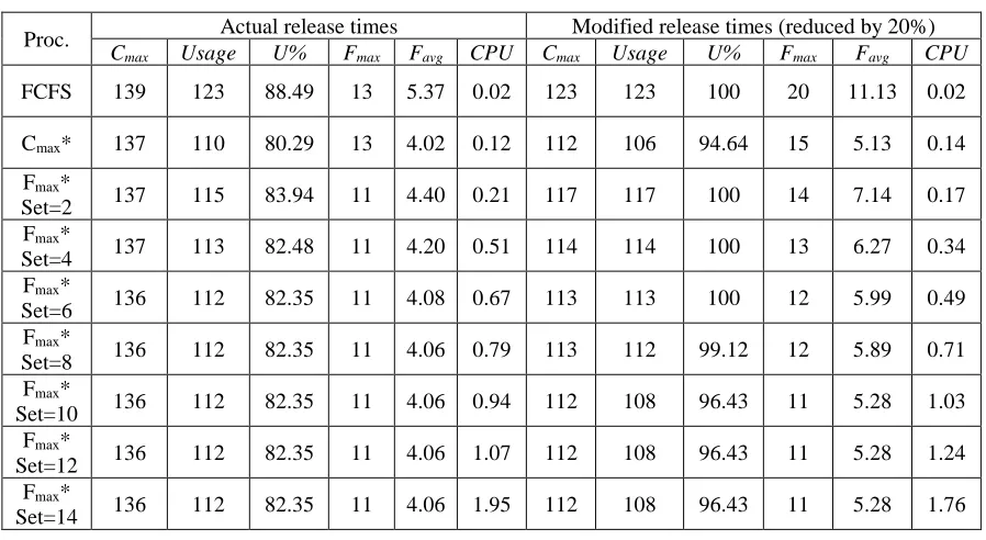
Table 13 Experiment Summary ... 36

Table 14 FAA Separation Requirements (in Minutes) ... 39

Table 15 Number of Possible Solutions for N = 12... 40

Table 16 Number of Possible Solutions for N = 16... 41

Table 17 Experiment Summary - Case 1: Actual Data with 1:5:4 Types Ratio ... 44

Table 18 Experiment Summary - Case 2: Actual Data with 2:4:4 Types Ratio ... 45

Table 19 Number of Possible Pairs for N Jobs ... 52

Table 20 Experiment Summary – Part (1): Actual Data (N = 100) ... 56

Table 21 Experiment Summary – Part (2): Actual Data with Type Ratio of 3:1 ... 56

Table 22 Experiment Summary – Part (3): Actual Data with Type Ratio of 1:1 ... 57

Table 23 Minimum Separation Time (in Minutes) ... 62

Table 24 Airport Traffic Summary for Top 30 Busiest Airports in USA (2015) ... 73

Table 25 JFK Airport Data ... 77

(10)

viii

LIST OF FIGURES

Figure 1 Hartsfield Jackson Atlanta International (ATL) Airport Diagram ... 2

Figure 2 Charlotte Douglas International (CLT) Airport Diagram ... 3

Figure 3 New York JFK International (JFK) Airport Diagram ... 3

Figure 4 Final Sequence for the Cmax Algorithm Example ... 18

Figure 5 Gantt Chart for the Counter Example ... 23

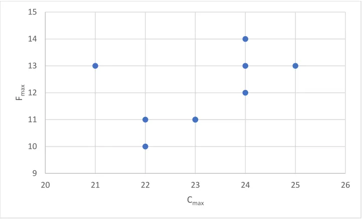
Figure 6 Candidate Optimal Solutions in XY Plot ... 30

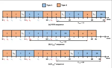
Figure 7 Gantt Chart for the Example ... 31

Figure 8 Number of Possible Solutions for N = 12 ... 41

Figure 9 Comparing Fmax Performance Using FCFS, Fmax* and Cmax* Approaches ... 46

Figure 10 Comparing Usage Performance Using FCFS, Fmax* and Cmax* Approaches ... 47

Figure 11 Performance vs Set Size for Case 2b (Types Ratio of 2:4:4 and Modified Release Time) ... 48

Figure 12 Dominant Solutions for Usage and Fmax (Case 2b) ... 48

Figure 13 Number of Departing Flights Every Hour at ATL ... 54

Figure 14 Comparing Fmax Performance Using FCFS, Fmax* and Cmax* Approaches ... 58

Figure 15 Comparing Usage Performance Using FCFS, Fmax* and Cmax* Approaches ... 59

Figure 16 Cmax* Approach Performance vs Set Size for Case 3 ... 59

Figure 17 Fmax* Approach Performance vs Set Size for Case 3 ... 60

Figure 18 Dominant Solutions for Usage and Fmax (Case 2) ... 60

(11)

1

Chapter 1 – Introduction

The runway scheduling problem (RSP) is a common problem at large airports. Airplanes

queue accumulate quickly for both takeoff and landing operations with limited runway

capacity. Delays occur and cause unwanted operational problems and unnecessary costs.

The main responsible party for controlling runway operations is the airport traffic control

tower (ATC). With many responsibilities at hand it is necessary to be able to operate as safe

as possible as a first priority, then other considerations can be dealt with such as operating

with minimum cost and/or maximum efficiency.

With the increased demand for flights over time, the capacity of many runways becomes

insufficient when running in a simple fashion such as first-come-first-served. It has become

important to use smart techniques to run the take-off and landing process more efficiently.

The problem of operating the runway efficiently is challenging and there are many issues that

cause this. One reason is the structure of the problem. The runway is the bottleneck of the

airport system (Idris et al., 1998). Many aircraft are ready to take off and many are ready to

land at the same time but the runway is a limited resource for handling these operations.

Also, there are strict operational standards enforced by the International Civil Aviation

Organization (ICAO) and the Federal Aviation Agency (FAA) to insure safety and other

issues. One such key standard is the time and distance separation requirement between

aircraft using the same runway. This varies between consecutive aircraft based on their size

and type of operation. Because of the sequence dependency involved, this makes the aircraft

sequencing problem (landing or taking off) an NP-hard problem (Bennell et al., 2013)

Another reason that makes the problem challenging is the time required to solve the problem

which must be very fast (near real-time) due to the nature of the problem (new events

occurring every minute). Even with the high technology resources available these days that

might be used to solve the problem, it might take a relatively long time to provide efficient

solutions.

There have been many efforts in the literature to solve the airport runway scheduling problem

(RSP), both on the landing (aircraft landing problem, ALP) and the take-off (aircraft takeoff

(12)

2

mixed integer programming (MIP), machine scheduling, the traveling sales man (TSP), and

queueing. Also, many solution methodologies have been considered such as dynamic

programming, branch and bound, heuristics and meta-heuristics (detailed literature review is

in Chapter 2). There is still room for improvement especially in the area of providing fast and

efficient solutions that can be implemented in practical environments.

There are several types of airport hubs in the United States according to the FAA. They are

Large, Medium, Small and Non-hub. There are 30 large hubs with passenger traffic ranging

from 16 million to 96 million passengers per year. Active runways range from one to five

(most commonly parallel), and each has a different geometrical configuration. Three

examples of large airports are Hartsfield Jackson Atlanta International Airport (ATL) in

Atlanta, GA (Figure 1), Charlotte Douglas International Airport (CLT) in Charlotte, NC

(Figure 2) and New York JFK International Airport (JFK) in New York (Figure 3). See

Appendix A for details.

(13)

3

Figure 2: Charlotte Douglas International (CLT) Airport Diagram

(14)

4

For the ATP, many considerations are important in solving real problem. The first is the

ability to model the system accurately relative to the real case. At any airport, each aircraft is

assigned a gate during its stay at the airport. There is a scheduled departure time for each

airplane to leave its gate. It is most preferable to leave the gate on schedule or even few

minutes early, if all passengers have boarded. Of course, the flight might leave after its

scheduled time too. Even when leaving the gate exactly on-time, there is a required time to

taxi from the gate to the runway and possible waiting time in a queue of aircraft waiting for

the runway to be cleared for takeoff. Having a model that captures these considerations is

important to help the ATC to make the aircraft sequencing decisions.An additional task for

ATC arises when there are multiple runways used for departure. In this case, runway

assignment must be considered first.

Another important issue is to consider the basic standards required in the system such as the

separation problem and definition of classes of aircrafts used by the ICAO. The separation

requirement is very important between consecutive airplanes using the runway for safety

reasons. When an airplane uses the runway to take off or land, a wake vortex is created from

the movement of the aircraft and it can impose dangerous control issues for the next airplane

using the runway. The effect of the wake vortex depends on both the size of the aircraft

involved and the type of operation (landing or takeoff). Aircraft are classified either small,

large or heavy. Large aircraft have larger wakes and thus require a longer separation time

from the next aircraft. One of the main tasks for the ATC is to insure the required separation

time between the aircraft using the runway for any given sequence. A standard minimum

separation time between different classes of airplanes is enforced by both the FAA and the

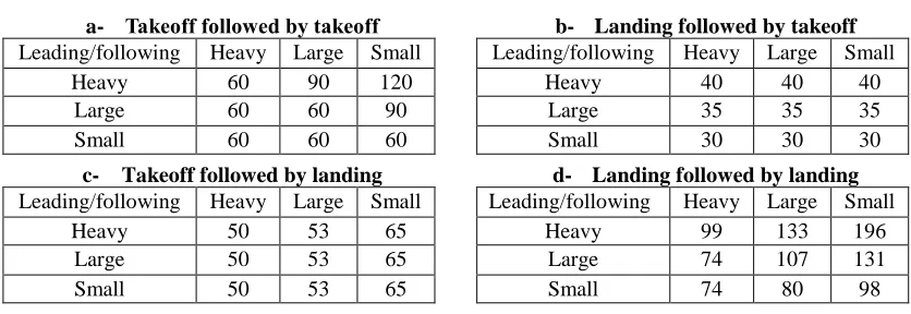
ICAO (summarized in Table 1).

One of the challenging issues regarding the ATP is defining the objective function, or the

performance measure, for the problem. There are many stakeholders in this system, some

with conflicting interests. An airline using the airport would prefer to have its flights leave

on time with least cost possible (minimum waiting time to take off), the airport authority

would prefer to have maximum throughput on its runways and achieve fairness among

(15)

5

Table 1: Minimum Separation Times (in Seconds) for Two Consecutive Operations

a- Takeoff followed by takeoff

Leading/following Heavy Large Small Heavy 60 90 120

Large 60 60 90 Small 60 60 60

b- Landing followed by takeoff

Large 35 35 35 Small 30 30 30

c- Takeoff followed by landing

Large 50 53 65 Small 50 53 65

d- Landing followed by landing

Large 74 107 131 Small 74 80 98

Finally, it is important to have a method that solves the problem in the most efficient way and

satisfies all of the stake holders. Also, it desirable to have the ability to solve the problem

dynamically, as the uncertain and fluid nature of the problem based on the actual push back

time, the taxi time, etc.

This dissertation is organized as follows. Chapter 2 is concerned with the literature and the

approaches have been taken by previous researchers. Chapter 3 introduces practical

approaches to solve the ATP problem for two types of aircraft using a single runway.

Chapter 4 introduces a practical approach to solve the ATP problem for three types of aircraft

using a single runway. Chapter 5 introduces a practical approach to solve the ATP problem

for two types of aircraft using two parallel runways. Finally, Chapter 6 concludes with future

(16)

6

Chapter 2 - Literature Review

In this chapter, we review the literature on the runway scheduling problem. In Chapter 1, it

was noted that the RSP, in general, is an NP-hard problem.

Although the main purpose is to maximize the efficiency of the system by improving the

utilization of scarce resource, airport runways in this case, some studies consider different

goals and different approaches to solve the problem. Different goals include minimizing the

summation of delays or minimizing the summation of penalties for deviating from target

landing time for the case of landing. Different models and solution approaches have been

used to solve the RSP. In section 2.1, papers that deal with the RSP are categorized based on

solution approaches with the emphasis on their objective functions and assumptions. In

section 2.2, we introduce the machine scheduling literature relevant to the RSP problem, with

the assumption of dependent setup times between different jobs, release times, and batching.

2.1 Runway Scheduling Problem Literature

The runway scheduling problem has been studied in the literature since the late 1970’s.

Psaraftis (1978) is one of the early studies in this area. Since then, different studies have

considered different models, assumptions and goals. Also, different methodologies have been

used to solve the RSP, for example dynamic programming, mixed integer programming,

genetic algorithms, and many others. The review paper by Bennell et al. (2013) divided the

area into two main categories based on the type of operation: aircraft landing problem (ALP),

and aircraft take-off problem (ATP). However, since then, more papers consider both

operations in the same model so it may be more appropriate to categorize by solution

approach first.

Dynamic programming (DP) is one of the common approaches that have been used in the

RSP. Because of the sequencing nature of the RSP problem, most cases can be modeled as a

dynamic programming. In general, the time complexity for solving a single runway problem

using DP is O(CNC), where N is the number of jobs and C is the number of aircraft classes

(Bennell et al., 2013).

Bianco et al. (1999) solved the landing problem for one runway as a single machine

(17)

7

model to minimize completion time. A dynamic programming formulation was used to find

a lower bound. Two heuristic algorithms were considered to solve the problem effectively

for real scenarios.

Balakrishnan and Chandran (2007) presented a new class of techniques based on dynamic

programming to optimize multiple objectives for a departure problem. They developed a

unified framework under constraint position shifting (CPS). Other constraints such as wake

vortex separation and runway crossing restrictions were considered.

Many other studies used dynamic programming to solve the problem. Psaraftis (1980),

Trivizas (1998), and Craig et al. (2001) used dynamic programming to maximize throughput,

while Lieder et al. (2015) used it to minimize delay. Many studies solved the ALP for

multiple objectives using DP. Bayen et al. (2004) and Brentnall (2006) considered both

throughput and delay for the ALP. Lee and Balakrishnan (2008), Balakrishnan and Chandran

(2010), and Bennell et al. (2016) solved the ALP for multiple objective functions using DP.

Some studies considered local search heuristics for part or for the whole algorithm. Dear and

Sherif (1989) is one of the early works that used a heuristic to maximize the runway

throughput for the ALP, while maintaining constraint position shifting (CPS). Bianco et al.

(2006) coordinates inbound/outbound traffic flows in the terminal and runway by using a job

shop scheduling model with both setup time and release time constraints. They represent

several operational constraints and runway configurations in a uniform framework. A

fast-dynamic local search heuristic algorithm is used for the job shop model considering different

performance measures. An experimental analysis for a real problem is considered.

Recently, Soomer and Frankx (2008), Furini et al. (2012, 2015), Sama et al. (2013, 2014,

2015), and Guepet et al. (2017) use heuristic methods to minimize the delay. Ma et al.

(2014), Ghoniem et al. (2014), Ghoniem and Farhadi (2015), and Sabar and Kendall (2015)

use heuristic methods in variant cases in the RSP for the same goal of minimizing the total

deviation from target times. One of the issues with heuristics is that they do not guarantee

optimality.

Another common approach in the RSP literature is genetic algorithms (GAs) and other

metaheuristics. Atkin et al. (2007) used a hybrid meta-heuristic algorithm to recommend a

(18)

8

throughput for the take-off scheduling problem with the restrictions of separation times,

controllers’ limitations, and geometrical constraints. A case for London Heathrow airport is

solved and compared to actual schedule performance.

Hancerliogullari et al. (2013) developed a priority rule for the mixed arrival and departure

scheduling problem with multiple runways. The problem was modeled as an identical

parallel machines scheduling model with release times, target and deadline times and

sequence dependent constraints to minimize the weighted tardy times. A meta-heuristic

(simulated annealing) was used to solve the problem and compared to optimal solutions for

small and medium instances.

Other researchers used GAs to solve the ATP and the ALP. Some researchers use it in

extended cases (e.g. multiple runways), as well. Beasley et al. (2001), Capri and Ignaccolo

(2004), Veidal (2007), and Yu et al. (2011) used GAs to minimize the total deviation from

target time for one runway landing cases. Stevens (1995), Ciesielsky and Scerri (1998),

Cheng et al. (1999), Hansen (2004), Hu and Chen (2005), Pinol and Beasley (2006), Xie et

al. (2013), and Zhou and Jiang (2015) employed GA for the ALP for two or more runways.

While it is popular to use a GA in the RSP problem, the computational requirement make it

difficult to find good solution in a reasonable amount of time.

Another common approach that have been used in the RSP is Mixed Integer Programing

(MIP). It has been used to solve the problem since the 1990’s. Beasley et al. (2000)

considered the landing problem for both single and multiple runways to optimize multiple

performance measures. A 0-1 MIP model using a tree search approach was used with

flexible formulation and two possible objective functions: minimizing the cost of deviation

from target time and maximizing throughput. A strong LP relaxation was developed to

determine a lower bound. A heuristic algorithm was developed to improve the computation

time. They solve up to 50 aircraft efficiently.

Anagnostacis et al. (2001) developed a framework for an automated decision aid to solve the

ATP by increasing capacity (maximizing throughput) and decreasing delay, while

Anagnostacis and Clarke (2003) considered maximizing runway utilization assuming the

sequence of runway events (arrival, departure, and crossing) is given. They used a two-stage

(19)

9

given the time for arrival and crossing events. An IP model is used for the second stage to

fill the departure events with the existing population of departing aircraft to maximize

throughput.

Gupta et al. (2009) used an MIP model with multi-objective functions to minimize overall

system delay, maximum individual delay, and maximize throughput for take-off. Both

separation requirements and optional time window constraints were considered. They also

considered different schemes for managing the queue area for the runway. A special case at

Dallas Fort Worth (DFW) Airport was studied and a modified model (more computationally

efficient) was presented.

Clare and Richards (2011) used an MIP model to optimize taxiway routing and runway

scheduling throughput for the ATP. They reduced the average taxi time by half compared to

first-come-first-served for a case at London Heathrow airport with up to 240 planes. An

efficient method that reduces the computation time without loss in performance was

introduced.

There are other studies considered using MIP or branch and bound methods to solve the RSP.

Brinton (1992), Abela et al. (1993), Ernst et al. (1999), and Beasley et al. (2004) focused on

minimizing total deviation from target times for landing aircraft. Wang et al. (2015) used

branch and bound to minimize multi objective functions for landing, while Ghoniem et al.

(2015), Vasilyev et al. (2016) and Avela et al. (2017) used an MIP to maximize runway

throughput for mixed operation (landing and takeoff) cases. In general, MIP tends to have

long computation times to reach an optimal solution. Also, as the number of aircraft becomes

larger, the solution process grows exponentially.

Other methodologies used include ant colony optimization, queuing theory, column

generation approach, simulation and constraint satisfaction. Van Leeuwen et al. (2002) used

constraint satisfaction to assist controllers in planning and scheduling the ATP. Using the

ILOG solver, an optimal departure schedule is found for maximizing throughput.

Randall (2002), Bencheikh et al. (2009), Feng et al. (2013, 2016), and Xu (2017) used ant

colony optimization to minimize the deviation from target landing time, while Wen et al.

(20)

10

and Bauerle et al. (2007) used queuing theory techniques, Brentnall and Cheng (2009) and

Soykan (2016) used simulation, Murca and Muller (2015) used an exact algorithm approach,

and Ma et al. (2016) used sparse optimization.

Some observations from the literature can be summarized as follow:

• RSP is an NP-hard problem. The presence of the separation time between different

classes is one of the main reasons.

• Most used solution methods are: dynamic programming, genetic algorithm, mixed integer programming, and local search heuristics.

• Most common objectives: minimizing completion time and minimizing tardiness.

• Few studies achieve multiple optimization goals or have the flexibility to solve the

problem for different goals.

• There is more literature about the ALP than the ATP. Most papers consider only one

type of operation although some recent papers considered both cases in the same

model.

• Most of the studies consider the static case while in reality, the RSP is dynamic. Since

the RSP is a real case problem that can be observed in many large airports worldwide,

it is desirable to have a solution that can be applied fast enough in the real cases while

providing good quality answers. This can help the airport tower controllers to make

better decisions.

Having these observations in mind, our goal is to solve the departure case runway scheduling

problem efficiently for multiple objectives in a dynamic environment.

In the next section, the literature is discussed for the machine scheduling problem, especially

those that share similarity with our model which is introduced in Chapter 3.

2.2 Single Machine Scheduling Literature

Because of the similarity between the machine scheduling and the runway scheduling

problem, machine scheduling models can be used for the runway problem. The runway can

be represented as a single machine while the aircraft can be represented as jobs to be

(21)

11

There may be (literally) thousands of papers written on machine scheduling. Also, many

review papers focusing on scheduling with specific constraints have been written. Allehverdi

et al. (1999, 2008), and Allehverdi (2015) reviewed scheduling problems with setup

considerations in different machine scheduling environments. Each paper divided the

problems into independent setup and dependent setup in one dimension and batches and no

batches in another dimension. Potts and Van Wassenhove (1992), Webster and Baker (1995),

and Potts and Kovalyov (2000) reviewed scheduling with batching. They divided the

problem into two main areas: family scheduling models and batching machine models.

Up to 2015, less than 80 papers considered having setup times and release times in various

spectrums of problems from single machine to job shop, dependent or independent setups,

and batch or non-batch format. Of those papers, few of them considered solving the problem

for a single machine with dependent setup times and release times, as in our models in

Chapter 3 and 4.

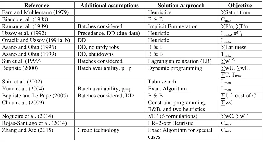
A summary table of the papers that considered dependent setup times and release times for a

single machine environment is shown in Table 2. The solution method, and the objective

function used in each paper is also shown in the table. A summary for each paper in the list is

provided in Appendix B.

To our knowledge, there is no similar work in the literature using the same methodology as is

(22)

12

Table 2: Summary for Single Machine Problems with Release and Dependent Setup Times Literature

Reference Additional assumptions Solution Approach Objective

Farn and Muhlemann (1979) Heuristics ∑Setup time Bianco et al. (1988) B & B Cmax

Raman et al. (1989) Batches considered Implicit Enumeration ∑F/n, ∑T/n Uzsoy et al. (1992) Precedence, DD (due date) Heuristic Lmax, #Uj

Ovacik and Uzsoy (1994a, b) DD Heuristic Lmax

Asano and Ohta (1996) DD, no tardy jobs B & B ∑Earliness Asano and Ohta (1999) DD, shutdowns B & B Tmax

Sun et al. (1999) Batches considered Lagrangian relaxation (LR) ∑wT2

Baptiste (2000) Batch availability, pj=p Dynamic programming ∑wU, ∑wC,

∑T, Tmax

Shin et al. (2002) Tabu search Lmax

Yuan et al. (2004) Batch availability, pj=p Exact Algorithm Lmax

Baptiste and Le Pape (2005) Batches considered, DD B & B ∑f, f=cost of C Chou et al. (2009) Constraint programming,

B&B, and two heuristics

∑wC

Nogueira et al. (2014) MIP (6 formulations) ∑wC, ∑wT Rojas-Santiago et al. (2014) LR+2-opt Heuristic Cmax

Zhang and Xie (2015) Group technology Exact Algorithm for special cases

(23)

13

Chapter 3 – Practical Approaches for Solving the Single Runway

Departure Sequencing Problem with Two Types of Aircraft

3.1 Introduction

In this chapter, the runway scheduling problem (RSP) is solved for take-offs (ATP) with one

assigned runway and two types of aircraft. All flights are known and on time. The required

time to travel from gate to runway is deterministic. Thus, the time when the aircraft is ready

to take-off is known. A separation time between take-offs is required for safety. The required

separation time varies between different types of aircraft as shown in Table 1 in Chapter 1.

The objective function is to find an efficient schedule for two performance measures:

minimizing completion time (Cmax), and minimizing maximum delay (Fmax). This facilitates

providing all solutions on a dominant solution curve, allowing a decision maker (the tower

controller) to implement schedules in near real-time.

These two objective functions are important measures in the RSP (de Neufville, 2016).

Completion time is an appropriate measure to satisfy the runway capacity. In the other hand,

maximum delay is an appropriate performance measure since fairness among different

aircraft is desired. Note that an optimal solution for maximizing throughput may not lead to

the optimal solution for minimizing maximum delay and vice versa.

There are a number of ways to find optimal solutions for the ATP. However, since the

problem is NP-hard, Computational time grows exponentially with the size of the problem

when using traditional optimization techniques (e.g. MIP and DP) as discussed in Chapter 2.

The proposed solution method in this chapter provides optimal answers for both objective

functions in a reasonable amount of time. There is also an opportunity to use the proposed

algorithm to solve the problem for large cases, by dividing the problem into small

sub-problems that can be solved separately.

In the next section, a scheduling model that represent the problem is introduced. Section 3.3

introduces a constructive approach to solve the problem for Cmax. Section 3.4 describes a

solution approach for minimizing Fmax that solve the problem in reasonable time for a small

case (up to 20 jobs), while section 3.5 is an extension to this approach to solve large cases. A

(24)

14

3.2 Scheduling Model

Machine scheduling models can be used for the runway problem because of the similarity

between the machine scheduling and the runway scheduling problem. The runway can be

represented as a single machine while the aircraft can be represented as jobs to be processed

on the machine. Before describing the problem via the scheduling model, some notation is

needed to describe the model.

3.2.1 Notation

Ci Completion time of job i (take-off). i = 1 … N.

Cmax Largest completion time or completion time of last processed job (Cmax = max{Ci})

Cmax* Minimum Cmaxof all possible sequences

Fi Flow time of job i. In the RSP, it is the time between the release time riand take-off

(Fi = Ci - ri).

Faverage Average flow time. Faverage = ∑Fi / N

Fmax Largest flow time. Fmax = max{Fi}

Fmax* Minimum Fmax of all possible sequences

mi Type of job i. In the RSP, it is the size of the aircraft (small, large, or heavy)

N Number of jobs

Nk Number of jobs from type k

pi Processing time for job i. In the runway scheduling problem pi = p for all i.

ri Release time of job i. The departure time from the gate plus the taxi time to the

take-off point

Sxy Setup time between a job of type x followed by a job of type y. In the RSP, it is the

required separation time between an aircraft of type x followed by an aircraft of type

y.

ti Starting time of processing job i. In the RSP, it is the time when the aircraft starts the

process of taking-off.

Usage Total time of runway usage (i.e. idle time is excluded). Usage = ∑p + ∑Sxy.

3.2.2 Problem Description

Consider the following scheduling problem. There are N jobs. There is a single machine.

(25)

15

two types of jobs, type 1, and type 2. If a type 2 job precedes a type 1 job, there is a setup

time S21 added after the processing of the type 2 job. If a type 1 job precedes a type 2 job,

there is no setup time. There is no setup time between jobs of the same type. All processing

times are known and constant.

The first objective is to identify a schedule that minimizes Cmax. The second objective is to

identify a schedule that minimizes Fmax. While minimizing Cmax is desirable, it may be

appropriate to identify schedules with larger Cmax, to minimize Fmax, as treating each job

(aircraft) fairly is also important. Thus, minimizing Fmax could be considered an alternative

(secondary) objective of the problem. As a consequence, considering multiple schedules is

important.

Clearly, if one ignores the release times ri, the optimal solution is to group jobs by type and

then schedule small aircraft followed by large ones (as that minimizes Cmax). However,

considering the release times, this approach may lead to idle time in the schedule.

When solving for Cmax, there may be multiple optimal solutions for Cmax. In this case, a better

candidate would be the one with less runway usage. Usage can be defined as total processing

time plus total setup (separation) time (i.e. idle time is excluded). Having lower runway

usage means more idle time, thus, more room for additional flights in the future.

Following the scheduling formulation α/β/γ as described in (Pinedo 2008) where α represents

the machine environment, β represents the processing characteristics and constraints, and γ

represents the objective to be minimized, the problem can be described as:

1/ {ri, S21, pi = p} / {Cmax, Fmax}, where 1 refers to the single machine environment.

(26)

16

Table 3: Problem description as a scheduling model

Real Problem Scheduling Model

• One runway • Single machine (N jobs)

• Two types of aircraft • Two job types (m1, m2) • Ready times (when aircraft ready to

take-off) are known.

• Each job i has release time ri

• Sequence dependent separation time between take-offs.

• Processing times p are known and constant

• If a type 2 precedes a type 1, a setup time S21 is added after the type 2 job • Otherwise no setup time

• Two objectives: Maximize throughput (Cmax), Minimize maximum delay (Fmax).

• Cmax = max{Ci},

Ci: Completion time of job i • Fmax = max{Fi},(Fi = Ci - ri)

3.3 A Constructive Method for Solving the ATP to Minimize Completion Time (Cmax) In order to solve the described scheduling problem in sec 3.2 for minimizing Cmax, a

constructive algorithm is used. Basic rules to build the algorithm are introduced first,

followed by algorithm description.

3.3.1 Build Up for the Method

Let ∑p = summation of process time for all jobs in a sequence, ∑S = summation of all

separation times required between jobs, and ∑d = summation of all idle times occurs

between jobs. Separation time occurs when switching from one type to the other according to

the definition of the problem. Idle time occurs when the machine is idle and next job has not

yet been released.

For 1/ {ri, S21, pi = p} / Cmax, Cmax = ∑p + ∑S + ∑d. Since ∑p is fixed, then minimizing Cmax

is equivalent to minimizing ∑S + ∑d. Since p=1, S= {0 or 1} and release times are integers,

the following rules minimize ∑S + ∑d:

1. Ordering each type jobs by their release time will minimize idle time in the problem.

2. If there are two job types available while the machine is idle, starting with the one

that needs less separation time will always reduce the number of setups in the

(27)

17

3. Sequencing jobs of the same type, if no idle time is left between them, will minimize

the setup time for the problem.

3.3.2 Minimizing Cmax Algorithm

Using the rules described above in the scheduling problem described in section 3.2.2, the

algorithm can be described as follows:

1. Start from t = r1 (where r1 is the release time of first available job in the problem)

2. Consider a list for all jobs available at time t, ordered by their release times:

a) If there is only one type of jobs available (Type 1 or 2), start with it.

b) If more than one type is available, start with a type 1 job.

3. Take the sequenced job out of the list.

4. Move to t = C[j] (where C[j] is completion time of last job in the sequence)

5. Update the list by considering all available jobs at time t = C[j]

a) If the first available job in the list after completion of job [j] is of the same

type of job j, then, sequence this job next.

b) If the first available job is not of the same type, then, if the first available job

from the same type has a release time less than or equal C[j] (for type 1) or C[j]

+ S21 (for type 2) sequence it after job j. Otherwise, sequence the first

available job from the other type.

c) If no jobs (from both types) are available, then move to t = rk, where k is the

first available job. Repeat step 2 for t = rk.

6. Repeat steps 2 to 5 until all jobs sequenced.

To illustrate how the algorithm works, consider the following example:

N = 10, p = 2, S21 = 1, S12 = 0, release times and types of jobs are in Table 4.

Table 4: Data for the Example for Minimizing Cmax Algorithm

Job # 1 2 3 4 5 6 7 8 9 10

Release time 0 0 2 4 6 7 8 10 11 13

(28)

18

At time t = 0, there are two available jobs: one of type 1, and one of type 2. In this case, the

type 1 job will be sequenced first. Next, at time t = 2 (completion time of first sequenced

job), there are two available jobs (2 and 3). Since the first available job (2) is not of the same

type as the sequenced job, we consider job 3. Since r3 is less than or equals C1, job 3 is

sequenced. Next, at time t = 4, there are two jobs of type 2 but no available type 1 jobs. In

this case, job 2 is sequenced after job 3. Repeating this process until all jobs sequenced will

lead to the sequence in Figure 4 with Cmax = 21.

Figure 4: Final Sequence for the Cmax Algorithm Example

Note that this approach does not consider minimizing Fmax in the first place. This means that

it is possible to obtain an optimal sequence for Cmax but not optimal for Fmax. Minimizing

Fmaxis considered in the next section.

3.4 An Exact Approach for Solving the ATP to Minimizing Maximum Delay (Fmax) In order to solve the described scheduling problem in sec 3.2 to minimize Fmax, an exact

algorithm is considered. The main idea of the algorithm is based on using the specific

characteristics of the ATP to identify a relatively small number of feasible solutions from all

possible solutions of the problem. From there, it is guaranteed that the optimal solution for

minimizing Fmax is within the identified candidate solutions.

For any scheduling problem, a solution is a sequence of jobs. One simple (but not necessarily

practical) way to find the optimal sequence is to enumerate all sequences and find the

optimal one. The number of possible sequences in this case is (N!), where N is the number of

jobs.

In Section 3.4.1 the necessary principles needed to build the algorithm are introduced.

(29)

19

3.4.3 explains the stopping criteria. Section 3.4.4 describes the algorithm, section 3.4.5

provides an example, and section 3.4.6 identifies the efficiency of the approach

3.4.1 Basic Principles to Build the Algorithm

For 1/ r / Cmax, ordering by release date (ORD) is optimal (Pinedo 2008). Since pj = p is a

special case, then ORD is also optimal for 1/ {r, pj=p} / Cmax.

Fmax can be considered as a special case of Lmax, with the due date for each job equals its

release time. It is known that ORD is not guaranteed optimal for 1/r/Lmax (Pinedo 2008).

However, for the case of 1/ r / Fmax, ORD is optimal. It is also optimal for 1/ {r, pj=p} / Fmax

Theorem 3.1: ORD is optimal for 1/ {r, pj=p} /Fmax.

Proof: Consider a schedule S where all jobs are ordered by release time. Considering only two adjacent jobs i and j in this schedule (pi = pj = p and ri < rj) where job i starts at time t,

Fmax (i, j) = max [Ci–ri, Cj–rj], noting that Ci = t +p and Cj = t +2p +k (where k = rj-Ci, if rj

>Ci, 0 otherwise), then Fmax (i, j) = max [t +p –ri, t+2p+k–rj].

Now, consider a schedule Sʹ where all jobs are ordered by release time except job i and j,

which have been reversed. Considering only jobs i and j in this schedule (pi = pj = p and ri <

rj) where job j starts before job i, then,

Fmaxʹ (i, j) = max [Cjʹ–rj, Ciʹ–ri], noting that Cjʹ= t +p +m, and Ciʹ= t+2p+m (where m = rj–t

if rj > t, 0 otherwise), then Fmaxʹ (i, j) = max [t +p +m –rj, t +2p +m –ri]

Now there are three possible scenarios:

1- If rj > Ci, then, rjis also greater than t (Ci > t), k > 0, m > 0 and m > k.

In this case, t +2p +m –ri is greater than both t +p –ri, and t +2p +k –rj.

2- If Ci > rj > t, then, k = 0 and m > 0.

In this case, t +2p +m –ri is greater than both t +p –ri, and t +2p –rj.

3- If rj < t then, k = 0 and m = 0.

(30)

20

In all three cases, Fmaxʹ (i, j) > Fmax (i, j). This means switching job i and j will never improve

Fmax for these two jobs. In addition, switching any two adjacent jobs may increase the

completion time for other jobs (as in case 1 and 2 above), which may make Fmax worse.

Thus, ordering all jobs by release time will optimize Fmaxfor any schedule. Q.E.D.

Going back to the runway problem, it means that if only one type of aircraft is considered,

then ordering them by release time will provide the optimal schedule for both Cmax and Fmax.

Notice that if 2 or more jobs have the same release time, it is optimal if they are ordered

arbitrarily.

Now consider the problem 1/ {ri, S21, pi= p} / {Cmax,Fmax} (described in section 3.2.2)

Theorem 3.2: for 1/ {ri, S21, pi= p} / {Cmax,Fmax}, If all jobs from type 1 must be processed first, followed by all jobs from type 2, or vice versa, then ordering each type of jobs by their

release time is optimal for Cmax and Fmax.

Proof: Consider the case where all type 2 jobs are processed first, followed by all type 1 jobs (note there is a setup time S21 between the two types).

Since it is not allowed to sequence any type 1 jobs before the type 2 jobs are sequenced, then

sequencing type 1 jobs is independent from sequencing type 2 jobs. Thus, ORD is optimal

for the first group (containing type 2 jobs), similar to 1/r/Cmax. Let the completion time for

this schedule called Cmax1.

For the second group (type 1 jobs), jobs cannot be processed until the completion of the last

type 2 job plus the setup time (S21). There are two cases. First, if all the release times of the

type 1 jobs (2nd group) are greater than Cmax1 + S21, then the two parts can be considered

separate problems. Therefore, ORD must be optimal for this group. In the other case, if

more than one job from type 1 has a release time smaller than Cmax1, then the two groups are

not separate. However, since it is restricted to start any job from the second group before the

completion of the first group, an adjusted release time (rjʹ) for the jobs that have a release

time smaller than Cmax1can be defined as: rj’ = Cmax1+S21. In this case, this part becomes

equivalent to the 1/r/Cmax, with possible multiple jobs having similar release times at the

(31)

21

Finally, consider the completion time for the whole problem, Cmax. Since both parts of the

problem can be optimal by ORD, it is clear that Cmax for the whole problem is optimal too.

Note that a similar argument can be used when starting with type 1 jobs followed by type 2

jobs (except setup time is zero). The same argument can be applied for the case of Fmax.

Q.E.D.

In general, when there are M types of jobs, M = {g1, g2, …, gm}, and all other assumptions are

the same, the following theorem can be stated.

Theorem 3.3: For 1/ {r, Sgh, pj = p} / {Cmax, Fmax}, where Sgh = setup time when type g job followed by type h job, if each type’s jobs must be processed together, then ordering each

group by its release times is optimal for Cmax and Fmaxregardless of the groups order.

Proof: Let M = {g1, g2…, gm} be the number of types. Without loss of generality, assume all jobs of type g1 are processed first, followed by jobs of type g2, and so on. From Theorem 3.2,

ORD is optimal for first group g1. It is also optimal for the 2nd group. All remaining groups

have similar situation to the 2nd group, therefore, ORD in each group is optimal for Cmax. The

same argument applies for Fmax. Q.E.D.

The next step is to develop a rule when one of the types (say type 1) is partitioned into two

separate groups. In this case, the machine will process the first group of the jobs of type 1,

then, it switches to process all the available jobs of type 2, then, go back to the first type and

process the rest of the jobs.

Partitioning one of the families (types) into two separate groups will add two new decisions:

1) What is the size of each group? and 2) Which group should each job be assigned? For the

second decision, a simple answer would be to assign the jobs based on their release dates (for

example if the first group contains k jobs, assign k jobs with the smallest release time to this

group). However, since the first and third group contains jobs from the same type, swapping

jobs between them will not add setup times in addition to those already exist in the sequence,

yet, it is not clear if swapping any jobs can improve the solution (i.e. assigning first k jobs

might not be optimal). A rule can be established in this case.

In order to establish a rule, consider the problem 1/r/Cmax. Assume the machine, besides

(32)

22

and a processing time. A setup time (S21) is needed when switching from processing jobs of

type 2 to jobs of type 1. Also, this job must be processed after processing k jobs of type 1.

This means that type 1 jobs will be partitioned into two separate groups with k jobs in the

first group and the remaining in the latter group. In this case, ORD for type 1 jobs is optimal

for Cmax, by assigning the first k jobs, ordered by their release times, to the first group and the

remaining jobs, ordered by their release times, to the latter group. The same holds for Fmax.

Theorem 3.4: Let {𝑟₁1, 𝑟₂1, … , 𝑟_𝑘1, 𝑟_𝑘+11 , … , 𝑟_𝑚1} be the release times of m jobs of type 1 such that 𝑟₁1 ≤ 𝑟₂1… ≤ 𝑟_𝑚1_{. Also, let 𝑟}

12 be the release time of a type 2 job.

For 1/ {r, S21, pj = p} / {Cmax, Fmax}. If the type 2 job must be processed after a specified

number (k) of jobs from type 1, then sequencing jobs with release times: 𝑟₁1, 𝑟₂1, … , 𝑟_𝑘1

,ordered by their release time, before the type 2 job and jobs with release times: 𝑟_𝑘+11 , … , 𝑟_𝑚1,

ordered by their release time, after the type 2 job is optimal for Cmax and Fmax.

Proof: Assume that the jobs with release times 𝑟₁1, 𝑟₂1, … , 𝑟_𝑘1 are assigned to the first group and jobs with release times 𝑟_𝑘+11 , … , 𝑟_𝑚1 are assigned to the latter group. Since all the jobs in

the first group must be processed before the jobs in the second group, it becomes equivalent

to the case described in theorem 3.3. Therefore, ordering jobs in each group by their release

time is optimal for Cmax.

From this result, swapping any job other than the kth_{from the first group with any job in the}

other group will not improve the performance (it will violate the ORD rule inside one or both

groups). Similarly, swapping any job other than the k+1th from the second group with any job

from the first group will not improve the performance. However, swapping job k from the

first group with job k+1 from the second group will not violate the ORD rule for each group

(or swapping jobs {k-1, k} with {k+1, k+2} and so on)

Notice that when swapping job k with job k+1, any setup times S12 and S21 will remain the

same. Notice also that all processing times are equal. This indicates that there will be no

effect on the performance due to the setup times and process times. Now, since 𝑟_𝑘+11 ≥ 𝑟_𝑘1,

swapping job k+1 with job k will never decrease the completion time of the first group

(depending on the position of 𝑟_𝑘1 and 𝑟_𝑘+11 on the timeline, the completion time might

(33)

23

decrease when swapping job k+1 with k. Thus, the completion time for the whole sequence

(Cmax) will never decrease. The same argument holds if swapping two or more jobs (e.g.

swapping jobs {k+1, k+2} with {k-1, k}).

This indicates that swapping jobs k and k+1 will never improve the performance of Cmax,

which also indicates that ordering by release time will guarantee optimality. The same

argument applies for Fmax. Q.E.D.

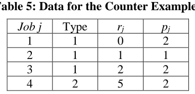
Note that if pi ≠ p, ordering type 1 jobs by release times, when a type 2 job must be processed

after k jobs of type 1, is not necessary optimal. Consider the following counter example (3

type-1 jobs and a type-2 job with release times and processing times as shown in Table 5.

Type-2 jobs must be processed after 2 type-1 jobs. S12 = 1, S21 = 0).

Table 5: Data for the Counter Example

Job j Type rj pj

1 1 0 2

2 1 1 1

3 1 2 2

4 2 5 2

If the type 1 jobs are ordered by release times, as shown in Figure 5(a), then, Cmax1 = 9 units.

However, a better solution with Cmax2 = 8 units is possible with the sequence {1,3,2} as

shown in Figure 5(b).

(34)

24

In the RSP, since the processing times are equal, the result obtained from Theorem 3.4 is

important for constructing the proposed exact algorithm. If the processing times are not

equal, DP can be used to solve the problem (Wang and Uzsoy, 2002).

In general, if more than one job of type 2 is in a middle group that partitions the family of

type 1 into two separate groups, then, the same rule above should apply as explained in the

next theorem.

Theorem 3.5: Let {𝑟₁1, 𝑟₂1, … , 𝑟_𝑘1, 𝑟_𝑘+11 , … , 𝑟_𝑚1} be the release times of m jobs of type 1, and

{𝑟₁2, 𝑟₂2, … , 𝑟_𝑛2_{} be the release times of}_n_{jobs of type 2 such that 𝑟}

11 ≤ 𝑟21… ≤ 𝑟𝑚1 and 𝑟12≤

𝑟₂2… ≤ 𝑟_𝑛2_.

For 1/ {r, S21, pj = p} / {Cmax,Fmax}, If a specified number of jobs (k) from type 1 must be

processed first, followed by all jobs of type 2, followed by the remaining jobs of type 1, then:

1) assigning jobs with release times 𝑟₁1, 𝑟₂1, … , 𝑟_𝑘1 to the first group and jobs with release times

𝑟_𝑘+11 , … , 𝑟_𝑚1_{to the third group, and}

2) ordering each group of jobs by their release time, is optimal for Cmax and Fmax.

Proof: Assume that the jobs with release times 𝑟₁1, 𝑟₂1, … , 𝑟_𝑘1 are assigned to the first group, ordered by their release times, and jobs with release times 𝑟_𝑘+11 , … , 𝑟_𝑚1_{are assigned to the}

third group, ordered by their release times, while the jobs of type 2 are assigned to second

group, ordered by their release times. In this case, from theorem 3.3, ORD in each group will

minimize the completion time of each group. Also, from theorem 3.4, swapping any jobs

from the first group and the third group will not improve the results if only one type 2 job is

in the second group. The same argument holds if more than one type 2 jobs are sequenced in

the middle group (the completion time might increase or remain the same but never decrease,

in any of the groups). Thus, the current sequence is optimal for Cmax. The same argument

holds for Fmax. Q.E.D.

Finally, Theorem 3.6 can be generalized for G partitions as stated in the next theorem.

(35)

25

For 1/ {r, S21, pj = p} / {Cmax,Fmax}, If the sequence is partitioned into G groups between the

two types, such that (m1) jobs from type 1 must be processed in the first group, followed by

(n1) jobs of type 2 in the second group, followed by (m2) jobs of type 1 in the third group and

so on, until the last group (G) with all the jobs assigned, then:

1) assigning jobs to each group according to their release time order, and

2) ordering each group of jobs by their release time, is optimal for Cmax and Fmax.

Proof: Assume all jobs are assigned to groups based on their release time order. From Theorem 3.4, ORD is optimal for Cmax in each group. From Theorem 3.5, swapping any jobs

between groups containing the same type of jobs will never improve the performance of

Cmax. Therefore, generalizing the case for G groups can hold for optimizing Cmax. Same

argument holds for Fmax. Q.E.D.

This means if the number of jobs in each group is specified, then, ORD in each group is

optimal for Cmax and Fmax. However, if the number is not specified then there is no simple

rule to solve the problem. This is the next step in the algorithm.

In general, when a specific sequence of groups is considered and each group contains a

specific number of jobs of one type, then, the setup times in the problem is controlled. This

means, any changes in the sequence will not eliminate setups.

Also, when the process times are all equal, then, regardless of any idle time occurrences

(because of the release times), the performance cannot be improved by swapping any jobs

between groups. So, instead of focusing on the release times or the setup time, we quickly

identify candidate solutions with a simple rule, and then evaluate each one by their

performance.

Note that if more than two types of jobs exist, the number of possible partitions will be much

larger as the problem grows. An alternative approach is to consider dynamic programming

(Wang and Uzsoy, 2002). However, because only two types of jobs are considered, it is easy

to identify all possible partitions of the scheduling problem. Identifying them is done in two

stages: 1) identify the number of groups/partitions, and 2) identify all possible number of

(36)

26

3.4.2 Identifying the Number of Possible Solutions

In order to describe the process of identifying the number of possible solutions the following

definition is introduced.

Definition 3.1: A sequence family contains all the sequences that have the same number of groups formed by the two types of jobs in the problem. For example, a sequence family for 3

groups contains all the sequences that may be formed by starting with the first type followed

by the second type followed by the first type (or start with the second type, followed by first

type, followed by second type) with all the possible number of jobs in each group.

The identification of possible solutions is done in two stages: 1) identify all the possible

sequence families, and 2) identify all candidate sequences that fit in each sequence family.

1) Identifying all possible sequence families:

Suppose there are N jobs (m1of these jobs are type 1 while m2 = N-m1 are type 2). A group

of jobs is defined as a number of jobs of the same type that are sequenced consecutively, and

with no job of the same type sequenced immediately before or after the group. Note that a

group can consist of one job if a job of one type is preceded and followed by jobs of another

type. Thus, for any sequence of jobs, there is only one possible way to identify the groups in

the problem. For example, a schedule with the following job types sequence {1, 1, 1, 2, 2, 1,

2, 2, 1, 1} has five unique groups.

From these outcomes, it is possible to define a sequence family from each group formation.

In order to find the number of all possible sequence families, there are two cases: (1) if the

number of jobs is equal for both types or (2) if the number of jobs is not equal. For both

cases, the minimum number of groups is two (one for each type of jobs). The maximum

number of groups when there is an equal number of jobs of each type is N (where N is the

total number of jobs and each group consists of one job only). Thus, the total number of

different sequence families is 2(N-1).

For the non-equal case, all sequence families from 2 to 2m groups are possible formations

(where m is the number of jobs from the type which has the least jobs). Since each sequence

family has two different scenarios (starting with type 1 or type 2), there will be at least 2(2m

(37)

27

ending with the jobs of the type with greater number of jobs, while having m groups of the

other type, each consists of 1 job. This makes the possible number of sequence families =

[2(2m – 1)] +1 = 4m – 2+1 = 4m – 1.

Identifying the number of sequence families is useful to identify the total number of

sequences in each family to be examined, which is discussed next.

2) Identifying the number of candidate sequences within each sequence family

When there are two types of jobs, the number of possible solutions for each sequence family

can be identified. There are two cases to consider: (1) when the number of jobs in each type

is equal and (2) when the number of jobs is not equal.

For the first case,

The number of solutions = 2*[∑ ( 𝑁 2 − 1

𝑖 − 1) (

𝑁 2 − 1

𝑖 − 1)

𝑁 2

𝑖=1 + ∑ (

𝑁 2 − 1

𝑖 − 1)

𝑁 2−1

𝑖=1 (

𝑁 2 − 1

𝑖 )] , N > 2

For the second case, let N1= number of jobs from type 1, N2 = number of jobs from type 2

𝑁₁′ = max⁡{𝑁1, 𝑁2} , 𝑁2′ = min⁡{𝑁1, 𝑁2}

The number of solutions =

2*∑ (𝑁1′− 1

𝑖 − 1 ) (

𝑁₂′_{− 1}

𝑖 − 1 )

𝑁2′

𝑖=1 + ∑ (

𝑁₁′− 1

𝑖 )

𝑁2′

𝑖=1 (

𝑁₂′_{− 1}

𝑖 − 1 ) + ∑ (

𝑁₁′_{− 1}

𝑖 − 1 ) (

𝑁₂′− 1

𝑖 )

𝑁2′−1

𝑖=1 , 𝑁2′ > 1

Table 6 compares the number of possible solutions using the group search algorithm versus

total enumeration, which is N!

Table 6: Computational Reduction for the Search Algorithm

No of jobs Search algorithm Total enumeration

8 70 40,320

12 924 4.79 E+8

16 12,870 2.09 E+13

20 184,756 2.43 E+18

3.4.3 Identifying a Stopping Criteria

When the search is ordered by number of groups, the value of Fmax follows a convex function

(38)

28

increases, the amount of setup time increases. At the same time, the amount of idle time may

decrease. The result is a convex curve. This result can be used to identify a stopping point in

the search as following: When the optimal value for Fmax for k groups is less than optimal

value for Fmax for k+1 groups, it means that Fmax for k groups is optimal for the problem.

Thus, the search can be stopped at this point.

3.4.4 Describing the Algorithms

The solution procedure is described as follows:

1- Determine the number of all sequence families for this problem (as described in

3.4.2)

2- Start with the sequence family of two groups starting with first type job followed by

the second type.

3- Using Theorem 3.6 to identify candidate sequences, consider all the sequences for

jobs that can fit within this sequence family (Note that for two-group sequence

family, starting with first type of job, only one sequence is possible. That is, to start

with all jobs from the first type ordered by their ready time followed by the jobs from

the second type ordered by their ready time. However, for more than two groups, use

the formula described in 3.4.2 - part 2 to count the number of all candidates)

4- Evaluate all candidate schedules in this sequence family and pick the one with best

solution as a candidate solution for this group formation.

5- If it is feasible, reverse the order of types while staying in the same sequence family

and repeat steps 3 to 4. Otherwise go to step 7.

6- For each sequence family pair, with the same number of groups, consider the best

solution of the two candidates.

7- Consider the next sequence family (by increasing the number of groups by one).

Repeat steps from 3 to 6.

8- Continue searching each sequence family pair until the candidate solution for the

current pair is larger than the candidate solution for the previous pair. Label the

candidate solution for the previous pair as S0 and the candidate solution for the