Multiscale Modeling of Plant Growth Combining Enzyme Kinetics and Whole Plant Dynamics and Experimental Design Applications.

ABSTRACT

REHM, KERI LEIGH. Multiscale Modeling of Plant Growth Combining Enzyme Kinetics and Whole Plant Dynamics and Experimental Design Applications. (Under the direction of H. T. Banks.)

While models of photosynthesis and physiological models of crop growth abound, the

ques-tions of how the productivity of photosynthesis drives plant growth and how the environ-ment (outside of PAR, CO2, and O2 availability [49]) affects these cellular level reactions

re-main largely unexplored. We construct two environment-dependent candidate model of plant

metabolism and growth based on previous work modeling the dark reactions of photosynthesis [49], light reactions of photosynthesis [28], and whole-plant metabolism [26], along with

informa-tion on carbon metabolism from [4] and [42] and whole-plant response to environmental factors

from [39]. The carbon uptake rate as predicted by the model is used to relate photosynthetic productivity with plant leaf area as predicted by a logistic growth model.

We use these models with a least-squares optimization algorithm to estimate parameters

that would replicate recorded growth of Arabidopsis thaliana [35] and soybean [39]. The leaf area predicted by the model agrees with the data and exhibits changes in behavior between

day and night. Moreover, metabolites involved in photosynthetic processes exhibit different

concentrations when exposed to daytime conditions or nighttime conditions. To investigate potential relationships between parameters in the models and overall model behavior, we use

a C3 cycle model [49] and one of the two constructed models to conduct further parameter

estimation problems and calculation of sensitivity matrices describing how much an equation changes when a parameter is varied some small amount from a predetermined value.

Additionally, we formulate a Fisher information matrix-based optimal design methodology

for the selection of the best state variables to observe and optimal sampling times for parameter estimation problems involving complex nonlinear dynamical systems. An iterative algorithm for

implementation of the resulting methodology is proposed. Its use and efficacy is illustrated on

© Copyright 2013 by Keri Leigh Rehm

Multiscale Modeling of Plant Growth Combining Enzyme Kinetics and Whole Plant Dynamics and Experimental Design Applications

by

Keri Leigh Rehm

A dissertation submitted to the Graduate Faculty of North Carolina State University

in partial fulfillment of the requirements for the Degree of

Doctor of Philosophy

Applied Mathematics

Raleigh, North Carolina

2013

APPROVED BY:

Lorena Bociu Ralph Smith

Hien Tran H. T. Banks

DEDICATION

BIOGRAPHY

The author spent her early childhood in the towns of Endicott, NY, and Poughkeepsie, NY, before moving to Cary, NC, at the age of 9 with her parents and two brothers. She graduated

from Green Hope High School in Morrisville, NC, in the top 1% of her class in 2004 and from Meredith College in Raleigh, NC, with a B.S. in Mathematics, B.A. in Religion and Philosophy,

and minors in Statistics and Computer Science, summa cum laude, in 2008. During her time at

Meredith College and at North Carolina State University, she has been very active in a variety of organizations, including service in the Meredith College Academic Technology, Lillian Parker

Wallace Lecture Series, and Sonia Kovalevsky Day committees and being an executive officer in

the University Graduate Student Association at North Carolina State University for 2.5 years in addition to being a leader in the worship ministry at her local church. When at home, she

ACKNOWLEDGEMENTS

I’d like to acknowledge the many people who have contributed to my successes over the past 26 years. My family and my husband, first and foremost, for their constant support, advice,

and encouragement in my academic and extracurricular pursuits. My friends, including my colleagues at North Carolina State University and those whom I consider my second family

through church, for reminding me to enjoy life – including my work. My many teachers over

the years who encouraged and inspired me to not only remain passionate about my education in but also take leadership roles in the classroom and in the community. My collaborators at

Syngenta Biotechnology, Inc., for their advice and input. And most certainly my Ph. D. research

advisor, for his guidance across several research projects and his mentoring as a mathematical researcher.

This research was supported by National Institute of Allergy and Infectious Diseases

(NI-AID) grant number R01AI07 1915-07, fellowships from the Center for Research in Scientific Computation (CRSC) and Center for Quantitative Sciences in Biomedicine (CQSB), and a

TABLE OF CONTENTS

LIST OF TABLES . . . vii

LIST OF FIGURES . . . viii

Chapter 1 Multiscale Modeling of Plant Growth Combining Enzyme Kinet-ics and Whole Plant DynamKinet-ics . . . 1

1.1 Introduction . . . 1

1.1.1 Physiology of photosynthesis . . . 2

1.1.2 Models of photosynthesis . . . 4

1.1.3 Physiological crop modeling . . . 8

1.1.4 Dynamical systems modeling and experimental design . . . 9

1.2 Proposed models . . . 11

1.2.1 Comprehensive model . . . 11

1.2.2 Compact light reaction model . . . 15

Chapter 2 Experimental Design for Vector Output Systems . . . 18

2.1 Introduction . . . 18

2.2 Mathematical Background . . . 19

2.2.1 Mathematical and statistical models . . . 19

2.2.2 Formulation of the Optimal Design Problem . . . 20

2.3 Standard Errors . . . 24

2.3.1 Asymptotic Theory for Standard Errors . . . 24

2.3.2 Clarification for plant growth model . . . 26

2.4 Numerical algorithm and optimization constraints . . . 26

Chapter 3 Numerical Results . . . 30

3.1 Parameter estimation . . . 30

3.1.1 C3 Model of [49] . . . 30

3.1.2 Modeling plant growth using the proposed models . . . 34

3.2 Sensitivity analysis of C3 model . . . 49

3.3 Experimental design . . . 56

3.3.1 HIV model . . . 56

3.3.2 HIV observable selection results, times fixed . . . 58

3.3.3 HIV observables and time point selection results . . . 62

3.3.4 C3 Cycle model [49] . . . 70

Chapter 4 Conclusion and Future Work . . . 87

4.1 Multiscale models . . . 87

4.2 Parameter estimation and sensitivity analysis . . . 88

4.3 Experimental design . . . 88

4.4 Concluding remarks . . . 90

APPENDICES . . . 96

Appendix A State variables and parameters . . . 97

A.1 State variables, descriptions, and initial values . . . 97

A.2 Parameters and values as labeled in [49] and [28] . . . 100

Appendix B Model equations . . . 105

B.1 C3 cycle reaction equations . . . 105

B.2 First-order light reaction equations from [28] . . . 109

B.3 Comprehensive model state variable differential equations . . . 111

LIST OF TABLES

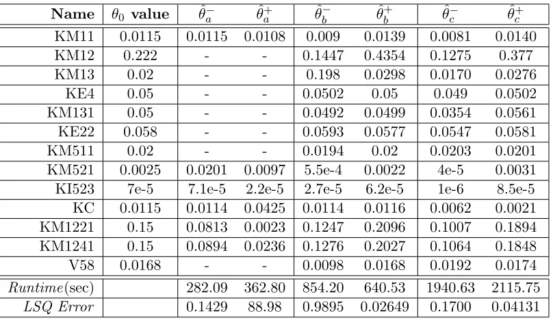
Table 3.1 θ0 and parameter estimates for top 13 parameters . . . 32

Table 3.2 Estimated~θ values for the models fittingA. thaliana data [35]. . . 35 Table 3.3 Estimated~θ values for models fitting Mead, NE, 2004 soybean data [39] . 41 Table 3.4 Predicted daytime metabolite concentrations . . . 45 Table 3.5 Values of parameters in the HIV model (3.1). . . 58 Table 3.6 D-optimal observables for the HIV model (3.2) using uniform sampling

times. . . 60 Table 3.7 E-optimal observables for the HIV model (3.2) using uniform sampling

times. . . 60 Table 3.8 SE-optimal observables for the HIV model (3.2) using uniform sampling

times. . . 61 Table 3.9 Standard errors of select parameters for the HIV model (3.2) using 35

optimally spaced sampling times and two optimal observables. . . 63 Table 3.10 Standard errors of select parameters for the HIV model (3.2) using 105

optimally spaced sampling times and two optimal observables. . . 67 Table 3.11 Optimal five observables and calculated asymptotic standard errors for

six parameters. . . 72 Table 3.12 Optimal ten observables and calculated asymptotic standard errors for six

parameters. . . 73 Table 3.13 Optimal five observables and calculated asymptotic standard errors for 18

parameters. . . 79 Table 3.14 Optimal ten observables and calculated asymptotic standard errors for 18

LIST OF FIGURES

Figure 1.1 Leaf tissue structure . . . 2

Figure 1.2 Plant cell structure . . . 3

Figure 1.3 Chloroplast structure . . . 4

Figure 1.4 Comprehensive model schematic . . . 13

Figure 1.5 Simplified model schematic . . . 16

Figure 3.1 CO2 uptake rates forθ0 and estimates ˆθa− and ˆθa+. . . 32

Figure 3.2 CO2 uptake rates forθ0 and estimates ˆθb− and ˆθ + b . . . 33

Figure 3.3 CO2 uptake rates forθ0and estimates ˆθ−c and ˆθ+c. . . 33

Figure 3.4 A. thaliana leaf area. . . 36

Figure 3.5 Model predictions of A. thaliana carbon uptake. . . 36

Figure 3.6 Model predictions of A. thaliana PC+ _{concentration. . . . 37}

Figure 3.7 Model predictions of A. thaliana RuBP concentration. . . 37

Figure 3.8 Model predictions of A. thaliana T3P concentration. . . 38

Figure 3.9 Model predictions of A. thaliana PGA concentration. . . 38

Figure 3.10 Model predictions ofA. thaliana T3Pc concentration. . . 39

Figure 3.11 Model predictions ofA. thaliana ATP concentration. . . 39

Figure 3.12 Model predictions ofA. thaliana ADP concentration. . . 40

Figure 3.13 Soybean leaf area. . . 42

Figure 3.14 Model predictions of soybean carbon uptake. . . 43

Figure 3.15 Model predictions of soybean PC+ concentration. . . 44

Figure 3.16 Model predictions of soybean RuBP concentration. . . 45

Figure 3.17 Model predictions of soybean T3P concentration. . . 46

Figure 3.18 Model predictions of soybean PGA concentration. . . 46

Figure 3.19 Model predictions of soybean T3Pc concentration. . . 47

Figure 3.20 Model predictions of soybean ATP concentration. . . 47

Figure 3.21 Model predictions of soybean ADP concentration. . . 48

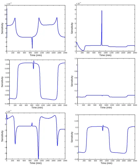
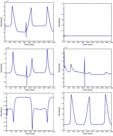
Figure 3.22 PQ sensitivity to select parameters . . . 51

Figure 3.23 RuBP sensitivity to select parameters . . . 52

Figure 3.24 Carbon uptake sensitivity to select parameters . . . 53

Figure 3.25 Sensitivity ofG(t) andS(t) to equation parameters. . . 54

Figure 3.26 Leaf area sensitivity to select parameters . . . 55

Figure 3.27 Solution of the log-scaled HIV model (3.2) with optimal 35 sampling times under constraint C2. . . 64

Figure 3.28 Solution of the log-scaled HIV model (3.2) with optimal 35 sampling times under constraint C3. . . 65

Figure 3.29 Solution of the log-scaled HIV model (3.2) with optimal 105 sampling times under constraint C2. . . 68

Figure 3.30 Solution of the log-scaled HIV model (3.2) with optimal 105 sampling times under constraint C3. . . 69

Figure 3.32 Solution of the C3 cycle model [49] with optimal 11 sampling times of five variables selected for six parameters under constraint C3. . . 75 Figure 3.33 Solution of the C3 cycle model [49] with optimal 11 sampling times of

ten variables selected for six parameters under constraint C2. . . 76 Figure 3.34 Solution of the C3 cycle model [49] with optimal 11 sampling times of

ten variables selected for six parameters under constraint C3. . . 77 Figure 3.35 Solution of the C3 cycle model [49] with optimal 11 sampling times of

five variables selected for 18 parameters under constraint C2. . . 83 Figure 3.36 Solution of the C3 cycle model [49] with optimal 11 sampling times of

five variables selected for 18 parameters under constraint C3. . . 84 Figure 3.37 Solution of the C3 cycle model [49] with optimal 11 sampling times of

ten variables selected for 18 parameters under constraint C2. . . 85 Figure 3.38 Solution of the C3 cycle model [49] with optimal 11 sampling times of

Chapter 1

Multiscale Modeling of Plant

Growth Combining Enzyme Kinetics

and Whole Plant Dynamics

1.1

Introduction

The development and refinement of dynamical systems models of photosynthesis reflect the

increased understanding of plant metabolism built through numerous in vivo, in vitro, and

even in silico experiments. These models typically address light-dependent reactions that occur within the thylakoid or light-independent reactions of the Calvin Cycle in the stroma and

cytosol; however, very few models address both sets of reactions - the exception being the work

of A. Laisk in [27] and [26]. The questions of how these reactions drive plant growth and how the environment (outside of sunlight, CO2, and O2 availability) affects these reactions remain

largely unexplored.

Utilizing the models of Zhu, et. al. [49], Lazar [28], and Laisk, et. al. [26], we construct two ODE candidate models of photosynthesis in C3 plants such as Arabidopsis thaliana, soybean,

and spinach. One candidate model, labeled the comprehensive model, uses a set of 74 first

order reaction equations developed in [28] to describe the light reactions. The other, labeled the compact model, utilizes four Michaelis-Menten enzyme kinetic equations to summarize these

reactions. Both models use the C3 cycle model of [49] as well as other mechanism descriptions

from [26]. We relate this cellular-level productivity to environmental conditions such as sunlight, CO2, and O2 availability and temperature by drawing upon mathematical models developed in

the area of crop modeling [39] and knowledge of how environmental factors affect photosynthesis

1.1.1 Physiology of photosynthesis

Photosynthesis is a process by which plants convert sunlight, CO2, and H2O into energy that is

usable by the plant and other organisms that may consume the plant. Photosynthesis primarily

occurs in the leaves of a plant. A leaf is composed of several layers of cells, as pictured in Figure 1.1. The cuticle, the outermost layer of a leaf is not cellular - it is a waxy protective layer. The

exterior layer of cells, the epidermis, controls the transaction of water, air, and other substances

into the leaf but does not contribute much to photosynthetic productivity. The body of the leaf, known as the mesophyll, contains the cells that perform photosynthesis.

Figure 1.1: Depiction of a cross-section of a leaf [48].

A leaf cell is composed of many organelles that perform specific tasks within a cell. The names and general locations of these organelles are pictured in Figure 1.2. Photosynthesis occurs

in the chloroplasts and cellular cytosol (also known as cytoplasm), and additional

energy-producing reactions occur in the mitochondria. The chloroplast, represented in Figure 1.3, further contains substructures that support photosynthesis and other cellular functions. The

light reactions of photosynthesis occur primarily in the thylakoid, which is a reaction center,

and the cholorplast stroma, a liquid-filled space between the thylakoid (and other structures) and the chloroplast’s membrane. The light-independent reactions, which are also known as the

When light strikes a leaf, it excites electrons contained in the thylakoid’s interior known

as the lumen. Once excited, the electron moves along an electron transport chain in which it slowly releases energy to power processes that occur along the thylakoid membrane. In

Pho-tosystem I, the movement of these electrons causes NADP+ to gain a negative charge and

attract a H+ atom to become NADPH. Names of NADP+, NADPH, and other metabolites involved in photosynthesis may be found in Section A.1 of the appendix. NADPH is used as a

hydrogen supplier to help reduce CO2 in the light-independent reactions. In Photosystem II,

electron movement instead creates a charge that moves H+ and supplies energy to the enzyme ATP synthase. When activated, ATP synthase catalyzes the combination of ADP and available

phosphate, Pi, into ATP. The bond between ADP and the newly added phosphate stores a

large amount of energy, which is used to fuel many other reactions in the cell.

Figure 1.2: Depiction of a plant cell with organelles labeled [46].

While the reactions of the C3 cycle don’t require light as a direct input, the rate of these

reactions is dependent upon the concentration of the products from the light reactions. The core reactions of the C3 cycle occur in the chloroplast stroma and utilize the ATP and NADPH

generated in the light reactions to create more stable energy storage metabolites in the form of

Figure 1.3: Depiction of a chloroplast with subsystems labeled [41].

other areas of the plant to fuel reactions and growth. Sucrose is generated in the cytoplasm and is primarily used to fuel processes in other areas of the same cell. Photorespiration, a process

that competes for the same resources that are used in the C3 cycle, dissipates the energy in

ATP and NADPH, and due to its high activity and impact on plant productivity, must also be considered when modeling the productivity of the C3 cycle. The reactions involved in the C3

cycle, sucrose production, and photorespiration are listed in [4] and [49].

1.1.2 Models of photosynthesis

The earliest steady-state models of C3 photosynthesis focus on key reactions involved in ATP, starch, and sugar generation and assume that most reactions exhibit Michaelis-Menten [29] type

dynamics (the primary exception being reactions catalyzed by RuBisCO). Farquhar, et. al. [20]

relate a leaf’s CO2 assimilation rate to radiance and temperature. Based on previous

knowl-edge gathered through experiments on chloroplasts harvested from spinach, eucalyptus, and

barley, the model calculates the rates of RuBP, ADP, ATP, NADP+, NADPH, and PGA

pro-duction and consumption based on electron transport that is fueled by radiance and controlled by temperature and atmospheric CO2 and O2. The model is tested at different atmospheric

concentrations of CO2 and O2 while varying the temperature and level of light absorbed by

the chloroplasts. While this model relates energy output to energy input with few equations, it

The C3 cycle model for the synthesis of sucrose and starch proposed by Laisk, et. al. [25]

is foundational to many current models. While much more comprehensive than [20], it makes assumptions that the NADPH:NADP+ _{ratio, UTP:UDP ratio, and total Pi remain constant}

and it removes the light-dependent reactions found in Laisk’s earlier work [27]. This model uses

20 ODE’s and 6 concentration balance equations to represent the dynamics of 23 state variables, including metabolite concentrations in the stroma and cytosol. Parameters are adjusted so that

the metabolite concentrations achieve a steady state indicative of that seen in experimentally

obtained data, and then the model’s performance is tested by varying atmospheric CO2 and O2

levels as well as maximum activity of ATP synthase. This model, while approaching the level of

complexity needed to model the Calvin cycle at the subcellular level, removes the environmental

factors of temperature (by assuming a constant temperature of 25◦ C) and radiance.

Pettersson and Ryde-Pettersson [31] propose a competing model for the C3 cycle at

equi-librium. Using Michaelis-Menten type dynamics for all reaction velocities, the model uses 16

ODES, 2 concentration balance equations, and 11 reaction equilibrium equations to describe the concentrations of 19 metabolites. This model is used to examine the effect of Pi concentration

on other metabolites’ concentrations. Like that of [25], this model shows great improvement in

modeling photosynthetic production, but the lack of environmental factors, assumptions made to enforce a steady state, and C3 reactions ignored by the model render it insufficient for in

silico experiments with varying environmental conditions.

Poolman, et. al [32] extend the model of [31] to include responses to the environmental

factors of Pi and light. Additionally, many of the steady-state assumptions are removed. The

assumptions used in this model are very similar to those of [25]: the NADPH and NADP+ concentrations are fixed, and level of light is reflected by varying the maximum activity of ATP

synthase instead of modeling the photosystems. The model is used to examine CO2

assimila-tion and starch producassimila-tion rates when the concentraassimila-tions of RuBisCO, SBPase, Pi, and triose phosphate translocator are varied.

The work by Zhu, de Sturler, and Long in [49] extends [25], [31], and [32] to reflect recent

advances in understanding of plant metabolism. In [49], the reactions for fructose and sucrose synthesis in the Calvin Cycle as well as those of photorespiration (not to be confused with

cellu-lar respiration) are quantified in terms of Michaelis-Menten enzyme kinetic equations (or simicellu-lar

mechanisms for reactions known to not fulfill Michaelis-Menten assumptions) and is one of the most comprehensive C3 models available, containing 31 state variables and 158 parameters.

The greatest weaknesses of this model are the conservation equations used to enforce constant

levels of phosphates, NADPH+NADP+, and ATP+ADP in the system. Parameters are found either in existing literature or estimated using a genetic algorithm, and then the model is solved

at varying levels of atmospheric CO2 and O2 to observe predicted carbon uptake rates.

model from [20] and extend it to the leaf level, where light intensity has a more pronounced

and nonlinear effect. In this later work, this model is expanded to better explain the effects of temperature change on the reaction rate equations and apply the model to canopy-level

systems, but does not include any more metabolites. While this model may be an acceptable

approximation of carbon fixation for plants in which the Calvin Cycle is not understood, models similar in scale to [49] may be preferable for species whose Michaelis-Menten constants are

available through previous research or may be estimated.

Similar to the efforts in C3 cycle modeling, a number of models have also been developed to describe the light reactions of photosynthesis. These reactions also influence the CO2 uptake

rate and O2 production [22] and produce ATP and NADPH necessary for fueling the C3 cycle.

Many of these models focus on chlorophyll fluorescence for the first second of exposure to light. Like CO2 uptake in the C3 cycle, chlorophyll fluorescence is a strong indicator of productivity

of the photosystems. During this small time frame, not all mechanisms of photosynthesis have

been activated; this simpler system composed of only the activated components is easier to model [22]. These models are then used to qualitatively compare long-term photosynthetic

performance (with the expectation that higher initial output implies higher long-term output).

The current generation of the foundational model by Laisk ([27], [25]) is described and used by Laisk in [26]. This model, while simpler than [49] in its description of the C3 cycle, includes

simple mechanisms to describe the photosystems, ATP generated by photophosphorylation, and the synthesis of some organic and amino acids. Parameters are experimentally determined using

intact leaves or taken from previous versions of the model, and then the model is used to explore

the effects of varying light and CO2 on the CO2 uptake rate. Like [49], this model also relies

on conservation equations to maintain constant concentrations of phosphates, ADP+ATP, and

PSI and PSII reaction centers. While this model’s quantitative description of the photosystems

is appealing and approximates long-term fluorescence yields, its simpler implementation of the C3 cycle may disagree with [49] in predicted metabolite concentrations.

In [22], Govindjee discusses the nearly 60 years of research that has been informative in his

efforts to model Chlorophyll (Chl)afluorescence. While he discusses many topics in his review, he expounds most upon the observed phases of fluorescence and their relation to

experimen-tally observed photochemical processes. He lists the several phases of fluorescence activity as

determined by local maxima and minima in fluorescence data and explains his proposed names and definitions of those phases (in an attempt to standardize the multiple naming schemes in

existence at the time of the paper’s creation). Then, using experimental findings from a number

of papers, he consolidates the knowledge of energy transfer between different reaction centers and the time scales on which these reactions occur after light is introduced. The timing of these

transfers is then compared to the fluorescence phases to link which electron transfers increase or

phase naming scheme of [22].

Zhu and Govindjee [50] construct an ODE model of PSII, cyt b6/f, and the OEC containing 20 state variables. The reactions included in the model are assumed to be bidirectional and are

mathematically described using first-order kinetics. While the model shows correlations between

the saturation of state variables and different fluorescence phases, the predicted fluorescence did not correspond well to observed fluorescence in both the start time of the fluorscense phase or

the level of fluorescense. This lack of fit may be attributed to parameters taken from literature

and not estimated using numerical optimization.

In [28], Lazar presents a model of PSI, PSII, cyt b6/f, FNR, and the OEC. While the electron

transfers that occur in the photosystems are catalyzed by enzymes like the C3 cycle, they

are written using a compartmental model and modeled using bi-directional first-order kinetic expressions. The model contains approximately 40 states and 20 parameters. Some parameters

are found in the literature, while others are estimated using least squares minimization. Lazar

then uses the model to investigate the rate of photosynthesis at different light levels. The timing of fluorescences phases as predicted by the model agrees well with observed fluorescence;

however, the levels of fluorescence were often overestimated by the model.

Rubin and Riznichenko [36] formulate a model of PSI, PSII, and cyt b6/f using a master equation approach. The parameters used in the model are primarily from literature, however,

some are manually estimated. While the model produces a qualitatively acceptable curve, the level of fluorescence predicted differed. The authors then propose a scheme based on Brownian

motion to model the movement of chemicals within reaction centers. Simulations are run to show

a model trajectory of a plastoquinone molecule; however, these results are not then related back to fluorescence levels.

Energy production in plant cells is not limited to photosynthesis - it also occurs in the

mitochondria through cellular respiration. In a recent review of current photosynthesis research, Amthor [4] calculates the number of photons needed to generate ATP. He considers percent of

useful radiation absorbed by plants, ATP generated in the C3 (and if applicable, C4) cycle,

and cellular respiration. He also estimates the amount of ATP used in starch building, mineral uptake, and protein synthesis. Amthor documents and balances the chemical reaction equations

for the C3 cycle, C4 modification, glycolysis, and the TCA cycle. While the equations are not

coded nor written as enzyme kinetics equations, they are easily converted should any additional mechanisms be needed to accurately model plant metabolism, and Michaelis-Menten constants

1.1.3 Physiological crop modeling

The field of physiological crop modeling approaches the question of predicting plant productivity

at a more tangible level: standard approaches in crop modeling relate crop yields or biomass

production to a plethora of environmental factors such as water, sunlight, soil nutrients, and crop management practices. The relatively simple Aquacrop model [43] utilizes basic mathematics

and patterns observed in plant growth to mainly relate plant growth to water consumption using

the formulaB =W P ×P

T r, whereB is biomass, W P is water productivity of the crop, and

T r is crop transpiration. As this model does not include factors that relate to carbon fixation

efficiency, it would be difficult to integrate this model with cellular-level kinetics models, but

it includes simple formulations about important ideas such as growth based on humidity and sunlight and the existence of canopy cover from neighboring plants, which inhibits growth.

The decision support system for agrotechnology transfer (DSSAT) [23] utilizes a modular algorithm and includes many more factors in plant growth and has been tested on about 16

crops in its history from 1988 to 2003. It utilizes the CROPGRO algorithm, which was originally

developed for soybean and peanut growth but has been successfully extended to wheat. The DSSAT program and its modular components are sold, so the source code or mathematics of

its current algorithm are not publicly available.

J. Jones, a developer of the DSSAT, however, has a history of investigating and mathemati-cally describing relationships between environmental factors and plant growth since the 1970’s.

In [33], the leaf area and biomass production of young individuals of several species of plants are

examined in three different temperature regimes. The first four weeks of growth of these species in each temperature regime was modeled using exponential curves with an acceptable fit. The

authors concluded that the plants of the same species in different temperature conditions grew

at different rates. Additionally, they observe that leaf area expansion and biomass production are directly related.

Plant growth at later periods of the seedling and vegetative stages, however, does not

fol-low an exponential pattern. At around the same time as [33], T. Sinclair was also developing a mathematical model that relates the basic environmental factors of temperature, available

water, nitrogen, and light levels to leaf area, biomass, and emergence of seeds. This model,

appearing in [40] in an application to modeling soybean growth, makes use of a system of simple mathematical equations to describe daily changes in plant size and weight for multiple

individuals of one species.

The mechanisms affecting leaf area change in soybean in [40] are expanded in [39], where the authors model how temperature and water availability affect leaf growth and senescence

function to relate to daily temperature to plant growth efficiency, allowing it to be used to

predict how plants will grow in different temperature regions. Like [40], this model also focuses on daily changes in plants; however, its formulation is very close to that of a system of ordinary

differential equations. The model is fit to three sets of soybean leaf area data, each covering the

120 days of plant development after emergence from the soil, with relatively successful results.

1.1.4 Dynamical systems modeling and experimental design

The application of a model to approximate trends seen in data raises many methodological

questions. Seber and Wild [44] provide an overview of the mathematical and statistical tools commonly used and refined by current research. While basic topics of different types of models

(such as linear ODEs, sigmoid and nonlinear functions, and even stochastic models) and

param-eter estimation techniques are covered, multiple aspects of analyzing and improving and model’s performance are also addressed. Additionally, [44] shows theoretical background to confirm the

reliability of these techniques, offers some explanations of the standard numerical algorithms

used to solve the parameter estimation problem, and discusses some of the common difficulties encountered in parameter estimation.

Banks and Tran [17] provide a primer on the basics of modeling and parameter estimation.

While it does not address the same breadth of mathematical and statistical modeling topics as [44], it is a very useful introduction to the concept and implementation of the iterative modeling

process to often-encountered situations in the physical and biological sciences. Banks and Tran

[17] contains several detailed examples of deriving a system of equations based on physical laws, performing an experiment that exemplifies the physical behavior, and analyzing how well the

model describes the experimental data using different mathematical and statistical tools. The

examples include heat conduction through a metal rod, sound wave propagation in an enclosed space, and size-structured population dynamics.

Inverse problem methodologies are discussed in [11] and earlier in [13] in the context of

dynamical system or mathematical model parameter estimation when a sufficient number of observations of one or more states (variables) are available. The choice of method depends on

assumptions the modeler makes on the form of the error between the model and the observations

(the statistical model). The most prevalent source of error is observation error, which is made when collecting data. (One can also consider model error, which originates from the differences

between the model and the underlying process that the model describes. But this is often quite

difficult to quantify.) Measurement error is most readily discussed in the context of statistical models. The three techniques commonly addressed are maximum likelihood estimators (MLE),

the variance of the data can be expressed as a nonconstant function. Uncertainty quantification

is also described for optimization problems of this type, namely in the form of observation error covariances, standard errors, residual plots, and sensitivity matrices. Techniques to approximate

the variance of the error are also included in these discussions.

Experimental design using the Fisher Information Matrix (FIM), which is based on sensitiv-ity matrices, is described in [12] for the case of scalar data. Sensitivsensitiv-ity matrices are composed

of functions that relate the change in a variable to the change in the parameter. The first order

quantifications of these relations are called traditional sensitivity functions and are useful in suggesting when a variable should be sampled to get the most information for estimating a

par-ticular parameter, especially when the first order sensitivity functions are used in conjunction

with the so-called second order sensitivity functions. This work also examines the usefulness of generalized sensitivity functions [45], which are calculated using the FIM, that are known

to describe how information about the parameters is distributed across time for each variable.

Both types of sensitivity functions are then used in [12] in numerical simulations to determine the optimal final time for an experiment of a process described by a logistic curve.

In [16], the authors develop an experimental design theory using the FIM to identify optimal

sampling times for experiments on physical processes (modeled by an ODE system) in which scalar or vector data will be taken. The experimental design technique developed is applied in

numerical simulations to the logistic curve, a simple ODE model describing glucose regulation and a harmonic oscillator example.

The use of mathematical models to better understand photosynthesis is featured in [6]

and [14]. Both works focus on applying the C3 cycle model of [49] to help determine a sam-pling regimen when performing an experiment, a topic of interest in the mathematical field of

experimental design. Multiple methods of selecting the optimal metabolites to measure in a

cellular-level experimental setting are discussed and evaluated in [6]. One method, which is an ad-hoc statistical method, determines which variables directly influence an output of interest

at any one particular time. A model using a subset of variables is determined via multivariate

linear regression, and the efficacy of the model is then measured using the Akaike Information Criterion. The variables that appear in the best models at the most time points are identified

as the most important to measure. Such a method does not utilize the information on the

underlying time-varying processes given by the dynamical system model. The second method, which utilizes the dynamics of the ODE model to determine what metabolites are most related

to parameters via a measure of parameter variability known as the Fisher Information Matrix,

is expanded upon and used [14] to include both metabolite and sampling time selection. Ex-tension of the second method first suggested in [6], based optimal design ideas, is the subject

of our experimental design algorithm development.

from [4], [26], and [39], and environmental data, to construct an environment-dependent model

of metabolism in plants including the light and dark reactions of photosynthesis. The carbon uptake rate A as predicted by the model is used to relate photosynthetic productivity with

plant leaf area as predicted by a logistic growth model. The model is fit to leaf area data

of Arabidopsis thaliana [35] and soybean [39] in separate numerical experiments to judge the

model’s ability to describe growth patterns in C3 species whose growth behavior and enzyme

kinetics have been largely quantified. While our current efforts compare the modeled leaf area

to leaf area data, our hope is to be able to use the experimental design methodologies of [6] and [14] with this proposed model in order to better design greenhouse and field studies of crop

performance based on mathematical predictions of overall plant performance under different

environmental conditions.

1.2

Proposed models

While many existing models either describe the macro-scale productivity of a plant via leaf area, biomass, or yield predictions or the micro-scale productivity of photosynthesis and CO2 uptake

rates, very few – if any – relate cellular productivity to gains in biomass using a mathematical

framework. The goal of our proposed model, which utilizes existing work by [26], [28], [39], and [49], is to accurately represent metabolic processes, in particular C3 photosynthesis, in leaf tissue

so that it may be used to predict photosynthetic productivity under varying environmental

conditions and reaction rates and relate this productivity to change in plant size. In order to distinguish between changes in productivity due to the environment and those due to genetic

regulation and variability, the model must also include mechanisms that reflect how external

factors such as sunlight, temperature, and water availability affect photosynthetic rates and plant development in addition to the Michaelis-Menten [29] mechanics that describe cellular

processes that fuel plant growth. Our initial conceptual model framework is pictured in Figure

1.4.

1.2.1 Comprehensive model

Our initial efforts focused on only modeling the individual-level dynamics of leaf area (Figure

1.4, right column). Different formulations of sigmoid functions, including the logistic equation and the Gompertz equation, were tested for their ability to fit leaf area data from [35] and [39]

in a least-squares minimization parameter estimation problem. Based on the resulting fits, we

dL

dt(t;~θ, ~E(t)) = dG

dτ

A(t;~θ, ~E(t))

Aopt

−dS

dτ !

dτ dT

dT dt

, L0=G(0) +S(0)

dG

dτ(t;~θ, ~E(t)) = rGG(τ) (1−G(τ)/kG), G0 =G(0) (1.1) dS

dτ(t; ~

θ, ~E(t)) = rSS(τ) (1−S(τ)/kS), S0 =S(0)

dτ dT(t;

~

θ, ~E(t)) =

 



2(T(t)−Tmin)α(Topt−Tmin)α−(T(t)−Tmin)2α

(Topt−Tmin)2α , Tmin

≤T(t)≤Tmax

0, T(t)< Tmin or T(t)> Tmax, (1.2)

whereL((t;~θ, ~E(t)) is the total leaf area of the plant,E~(t) is a vector of environmental forcing

functions,G(t;~θ, ~E(t)) is the expanding leaf area, S(t;~θ, ~E(t)) is the senescing plant leaf area,

and A(t;θ, ~~ E(t)) is the CO2 uptake rate based on the enzyme kinetics reactions (held constant

atA(t;~θ, ~E(t))/Aopt = 1 in the exploratory phase of model development). Explanations of the

parameters are available in Section A.2 in the appendix. The model includes a mechanism

τ(T(t)) as described by (1.2), taken from [39], that describes the influence of temperature on

growth and senescence rates; however, when this model was fit to the LAI data found in [39] of

two different plantings of the same type of spinach, the growth and senescence parameters of the models best describing these data sets changed by 10 – 30%. This indicates that temperature is

not the only factor that introduces variability into plant growth rates – factors such as genetic

variability and other environmental conditions may also affect a plant’s development.

When environmental information is not considered (or held constant for the duration of the

in silico experiment), the metabolite concentrations predicted by the model quickly stabilize.

The CO2 uptake rate quickly (within minutes) achieves a steady state that is not influenced

by temperature or captured radiance (see [49] and [6] for solutions of the C3 model). Thus

the CO2 uptake mechanism effectively scales the growth curve of (1.1) by a constant when

environmental conditions are not varied. Based on the models of [39], [40], and [49] - as well as basic knowledge about photosynthesis as described earlier in this chapter and information from

[4] - we include in our model the external factors of light intensity, temperature (in degrees

Celsius), atmospheric CO2 and O2 concentrations, and relative H2O availability (Figure 1.4,

left column). These factors are denoted as E~(t) = [r(t) T(t) [CO2] [O2] w(t)] and shown

in the left column of 1.4.

Similar to [26] and [49], gas solubility equations are used to calculate the concentration of CO2and O2in the plant based on atmospheric composition. Using Henry’s law for gas solubility,

Figure 1.4: Schematic of how multiple existing models are combined for a comprehensive quan-tification of photosynthesis and then related to environmental factors and biomass change.

(the interior of leaf cell) may be described by

[G] = P(elev)MG

KHP C(298.15, G)exp

h

−CG

1

T(t)+273.15− 1 298.15

i, (1.3)

where P(elev) is the pressure in atmospheric units (atm), MG is the mole fraction of gas in

the gaseous mixture, KHP C and CG are constants, and T(t) is the temperature in degrees

Celsius at time t. Assuming the atmosphere is an ideal gas, MCO2 = 0.00039 (390 parts per

million) andMO2 = 0.20946. The values of the other constants areKHP C(298.15,CO2) = 29.41,

KHP C(298.15,O2) = 769.23,CCO2 = 2400, andCO2 = 1700. We assume that the plant is grown

in an environment with sufficient nutrient availability, soil drainage, and pest control so that these factors would not impact plant development.

Reconstructing the model of the light reactions [28] to include environmental factors is

straightforward. The parameters kL1 and kL2, which describe the rates of light-induced

reac-tions, were changed to kL1r(t) and kL2r(t), where r(t) is the radiance at time t scaled such

thatr(t) = 1 corresponds to 3000 µmol m−2 s−1 of photosynthetically active radiation (PAR) and r(t) = 0 corresponds to 0 µ mol m−2 _s−1 _{PAR, so that dynamic sunlight levels may be}

used to vary the rate of the light reactions. If knowledge about light intensity under the canopy

increasing r(t) when the data is interpolated to form a function.

The reaction implemented to reflect the transition from S4 toS0 in the OEC is scaled by

w(t), which is relative water availability ( w(t) < 1 if there is a water shortage and w(t) = 1

if there is sufficient or abundant H2O). As the influence of temperature on the light reactions

is not very well understood, theτ(T) individual-level mechanism is assumed to be sufficient in scaling plant response rates; however, the study of Hill activity in [30] may serve as a useful

reference for future changes to the model in this area.

As the intent of [49] was to study the effect of different atmospheric concentrations of CO2

and O2 on carbon uptake rate, modifying the C3 cycle and photorespiration models to include

environmental conditions is also straightforward. Changes in CO2 and O2 concentration due to

environmental conditions are calculated by (1.3). H2O availability affects reactions involving

fructose-bisphosphatase (EC 3.1.3.11) and phosphoglycolate phosphatase (EC 3.1.3.18), and so

the velocities of these reactions are scaled by water availability w(t). The influence of

tem-perature on the Calvin cycle is also not very well understood, and so we assume the τ(T) individual-level mechanism and the changes in gas solubility at different temperatures are

suf-ficient mechanisms to describe plant response to temperature during a typical growing season.

Equations from the models of [26], [28], and [49] are used to calculate the CO2 uptake rate

A(t;~θ, ~E(t)), which is a commonly used measure of photosynthetic productivity. While many of

the proposed models in the literature suggest mechanisms that are appropriate for the systems they reflect and describe portions of plant behavior, we choose to build our cellular level enzyme

kinetics model using the C3 model of [49] and the light reactions model of [28] because they

include the most mechanisms. The models are linked using the photophosphorylation model of [26] to convert ADP to ATP and the production of NADPH from NADP+ _by

ferredoxin-NADP+-oxidoreductase (which was intentionally neglected in the model of [28] for simplicity).

By combining these models we remove the conservation equations for ADP, ATP, NADP+, and NADPH in [49].

The models of PSI, PSII, cyt b6/f, FNR, and the OEC from [28] remain mostly unchanged.

The equations of [28] are listed in Sections B.2 and B.3 of the appendix, and parameters as taken from [28] and tuned to enable the model solution to remain physically feasible are listed

in Section A.2 in the appendix. Instead of using a four-stage model (using stages S0 - S3) of

the OEC, we add stage S4 to expand it to a five-stage model that includes the splitting of H2O

to introduce more electrons and protons (H+) into the chloroplast. The concentration of H+ is

quantified in this model because it is required for the components of the model from [26]. This

requires altering some components of the light reaction model from [28], wherein a plentiful supply of H+is assumed. Finally, the generation of NADPH from NADP+during the oxidation

of FNR is added, and the reaction equation is changed to scale with NADP+ concentration so

The photophosphorylation mechanism of [26], transport of H+ across the thylakoid

mem-brane due to the oxidation and reduction of plastoquinone, and changes in NADP+, NADPH, and H+ _{in the stroma due to FNR are used to connect the light reactions inside the thylakoid}

lumen to the dark reactions that occur in the chloroplast stroma. Photophosphorylation is

modeled as

v11(t;~θ, ~E(t)) =

V11

x11y18+_k x8

E0(x88/x89)kHA

kM11,1kM11,2

1 + x11

kM11,1 +

y18

kM11,2 +

x8

kM11,3 +

x11y18

kM0,1kM0,2

, (1.4)

where variables are defined in Section A.1 and parameters are defined in Section A.2 in the

appendix.

All reaction equations formulated in [49] are used to model fructose and sucrose synthesis

as well as photorespiration except for the reaction that approximates photophosphorylation

(reaction 16 in [49]), which is replaced by (1.4). Additionally, we continue to use the balance equations of pentose phosphates, hexose phosphates, and inorganic phosphates to reduce the

number of states for which we must calculate via differential equations. Like [49], the current

model also holds the concentration of combined UDP and UTP constant because UTP is gen-erated in the reactions of cellular respiration (which are not included in our model). Variables,

parameters, and equations from [49] used in the current model may be found in Sections A.1, A.2, B.1, and B.3 in the appendix.

1.2.2 Compact light reaction model

As the dynamics of the light reactions are difficult to measure, the fine details included in the

model of [28] would be difficult to confirm using data. Additionally, because of its complexity, the model of [28] adds a significant amount of time to the calculation of one forward solution to

the model as compared to solving the C3 model of [49] alone. Therefore, replacing this model

with a simpler mathematical description of the light reactions (as depicted in Figure 1.5, center column) to reduce computational time would not negatively impact our ability to use available

metabolite data in parameter estimation problems.

Based on numerical experimentation with the comprehensive model, we alter the conceptual model (Figure 1.4) and temperature response functions used in this model. The temperature

re-sponse functionτ(T(t)) used to describe temperature’s response to both growth and senescence

in the comprehensive model is changed to τG(T(t)), that is, a temperature response function for growth only. A separate function for describing the dependence of senescence on

tempera-ture,τG(T(t)), is introduced. This senescence temperature response function is also from [39]. The set of equations describing change in leaf area and temperature response for this alternate

dL dt =

dG dt

A(t;~θ, ~E(t)

Aopt

−dS

dt, L0 =L(0) dG

dt = rGG(τG(T(t))) (1−G(τG(T(t)))/kG)

dτG

dT dT

dt

, G0 =G(0)

dS

dt = rSS(τS(T(t))) (1−S(τS(T(t)))/kS)

dτS

dT dT

dt

, S0 =S(0) (1.5)

dτG

dT dT

dt =  



2(T(t)−Tmin)α(Topt−Tmin)α−(T(t)−Tmin)2α

(Topt−Tmin)2α , Tmin

≤T ≤Tmax

0, T < Tmin or T > Tmax

dτS

dT dT

dt = (

0, T(t)≤Tmin

(T −Tmin)/Topt, T(t)> Tmin.

(1.6)

Figure 1.5: Schematic of how existing models of the Calvin Cycle and photophosphorylation are combined with a new, simple model of the light reactions and then related to environmental factors and biomass change.

The first-order reaction equations for the light reactions formulated in [28] and used in the comprehensive model are entirely replaced with four Michaelis-Menten chemical kinetic

[42]:

2H2O + 2PQ → O2+ 2PQH2 (1.7)

PQH₂+ 2PC++ 2H+_S ↔ 2PC + PQ + 4H+_L (1.8)

PC + Fd → PC++ Fd− (1.9)

Fd−+ H+_S +N ADP ↔ 2Fd + NADPH (1.10)

These summary equations correspond to the OEC and PS II (1.7), PC and cyt b6f (1.8),

PS1 (1.9), and FNR and Fd (1.10). Reversibility of (1.8) and (1.10) were confirmed by

informa-tion stored in BRENDA [37], an enzyme database. The corresponding Michaelis-Menten type equations are

v37(x, t, ~θ, ~E(t)) =

V37·PQ·r(t)·w(t)

km37+ PQ

(1.11)

v38(x, t, ~θ, ~E(t)) =

V38km−1381k

−1

m382





PQH·PC

+₋ PC·PQ

ke38

H_S+

H+ L 2   

1 +PQH2

km381 +

PC+

km382 +

PC

km383 +

PQ

km384 +

PQH·PC+

km381km382 +

PC·PQ

km383km384

(1.12)

v39(x, t, ~θ, ~E(t)) =

V39·PC·Fd·r(t)

(km391+ PC)(km392+ Fd)

(1.13)

v40(x, t, ~θ, ~E(t)) =

V40k−m1401k

−1

m402(Fd

−_{·NADP−Fd·NADPH/k}

e40)

1 +_kFd−

m401 +

NADP

km402 +

Fd

km403 +

NADPH

km404 +

Fd−·NADP

km401km402 +

Fd·NADPH

km403km404

,

(1.14)

whereV37,V38,V39, andV40are the reaction maximum velocities,ke38 andke40 are equilibrium

constants (ke38 is modulated with a proton gradient-type mechanism much like the

mathemat-ical description of ATP synthase [26]), and all km’s are Michaelis Menten constants.

All other model components remain unchanged between the two models. The compact

model, descriptions of all state variables and parameters, values of parameters and initial values

of state variables (values at time t = 0), equations from [49], and equations from [28] are included in Appendices B.4, A.1, A.2, B.1, and B.2, respectively. Parameter estimation for these

two models and sensitivity analysis on select parameters in these models using the methods

Chapter 2

Experimental Design for Vector

Output Systems

2.1

Introduction

In many scientific fields where mathematical modeling is utilized, mathematical models grow

increasingly complex, containing possibly more state variables and parameters, over time as the underlying governing processes of a system are better understood and refinements in

mech-anisms are considered. Additionally, as technology invents and improves devices to measure

physical and biological phenomena, new data become available to inform mathematical model-ing efforts. The world is approachmodel-ing an era in which the vast amounts of information available to

researchers may be overwhelming or even counterproductive to efforts. We explore a framework

based on the Fisher Information Matrix (FIM) for a system of ordinary differential equations (ODEs) to determine when an experimenter should take samples and what variables to measure

when collecting information on a physical or biological process that is modeled by a dynamical

system.

Building on the modeling and experimental design theory described in Chapter 1 and efforts

in [6], we formulate a previously unexplored optimal design problem to determine not only

the optimal sampling variables out of a finite set of possible sampling variables but also the optimal sampling time distribution given a fixed final time. We compare the SE-optimal design

introduced in [12] and [16] with the well-known methods of D-optimal and E-optimal design on a six-compartment HIV model [2] and a thirty-one dimensional model of the Calvin Cycle [49].

Such models where there may be a wide range of variables to possibly observe are not only ideal

2.2

Mathematical Background

2.2.1 Mathematical and statistical models

We explore our experimental design questions using amathematical model

d~x

dt(t) = ~g(t, ~x(t;θ~), ~q), t∈[t0, tf] (2.1) ~

x(t0;~θ) = ~x0

where~x(t;~θ) is the vector of state variables of the system generated using a parameter vector

~

θ = (~x0;~q) ∈Rp,p =m+r, that contains m initial values and r system parameters listed in

~

q,~g is a mapping R1+m+r → Rm, t0 ≥0 is the initial time, and tf <∞ is the final time. We

define anobservation process

~

f(t;~θ) =C~x(t;~θ), (2.2)

whereC is an observation operator that mapsRm →RN, where N is the number of variables

observed at a single sampling time. If we were able to observe all states, each measured by a different sampling technique, then N =m and C =Im×m_{; however, this is most often not the} case because of the impossibility of or the expense in measuring all state variables. In other

cases (such as the HIV example below) we may be able to directly observe only combinations of the states.

In order to discuss the amount of uncertainty in parameter estimates, we formulate a sta-tistical model [11] of the form

~

Y(t) =f~(t;~θ0) +E~(t), t∈[t0, tf], (2.3)

where~θ0 is the hypothesized true values of the unknown parameters and E~ is a vector random

process that represents observation error for the measured variables. We make the standard assumptions:

E(E~(t)) = ~0, t∈[t0, tf],

Var(E~(t)) = V0(t) = diag(σ0,1(t)2, σ0,2(t)2, . . . , σ0,N(t)2), t∈[t0, tf],

Cov(Ei(t)Ei(s)) = σ0,i(t)2δ(t−s), s, t∈[t0, tf],

Cov(Ei(t)Ej(s)) = 0, i6=j, s, t∈[t0, tf],

~

y(t) =f~(t;~θ0) +~(t), t∈[t0, tf].

When collecting experimental data, it is often difficult to take continuous measurements of

the observed variables. Instead, we assume that we havenobservations at timestj,j= 1, . . . , n,

t0 ≤t1< t2< . . . < tn≤tf. We then write the observation process (2.2) as

~

f(tj;~θ) =C~x(tj;~θ), j= 1,2, . . . , n, (2.4)

the discrete statistical model as

~

Yj =f~(tj;~θ0) +E~(tj), j= 1,2, . . . , n, (2.5)

and a realization of the discrete statistical model as

~

yj =f~(tj;~θ0) +~(tj), j= 1,2, . . . , n.

If we were given~θ0, we could solve (2.1) for~x(t;~θ0), a process known as solving theforward

problem. Alternatively, if we had a set of data~yj, j = 1,2, . . . , n, we could estimate ~θ0 in a

process known as solving the inverse problem. We will use this mathematical and statistical framework to develop a methodology to identify sampling variables that provide the most

information pertinent to estimating a given set of parameters and the most informative times at which the samples should be taken.

2.2.2 Formulation of the Optimal Design Problem

Several methods exist to solve the inverse problem. A major factor [11] in determining which method to use is additional assumptions made aboutE~(t). It is common practice to make the

assumption that realizations of E~(t) at particular time points are independent and identically

distributed (i.i.d.). If, additionally, the distributions describing the behavior of the components ofE~(t) are known, then maximum likelihood methods may be used to find an estimate of~θ0. On

the other hand, if the distributions forE~(t) are not known but the varianceV0(t) (also unknown)

is assumed to vary over time, weighted least squares methods are often used. We propose an optimal design problem formulation using a generalized weighted least squares criterion.

LetP₁([t0, tf]) denote the set of all bounded distributions on the interval [t0, tf]. We consider

the generalized weighted least squares cost functional for systems with vector output

JW LS(~y, ~θ) =

Z tf

t0

where P1(t) ∈ P1([t0, tf]) is a general measure on the interval [t0, tf]. For a given continuous

data set ~y(t), we search for a parameter ˆθthat minimizes JW LS(~y, ~θ).

We next consider the case of observations collected at discrete times. If we choose a set of

ntime points τ ={tj},j = 1,2, . . . , n, wheret0 ≤t1< t2< . . . < tn≤tf and take

P(t) =Pτ = n

X

j=1

δtj, (2.7)

whereδarepresents the Dirac delta distribution with atom ata, then the weighted least squares criterion (2.6) for a finite number of observations becomes

J_{W LS}n (~y, ~θ) = n

X

j=1

[~y(tj)−f~(tj;~θ)]TV0−1(tj)[~y(tj)−f~(tj;~θ)].

To select a useful distribution of time points and set of observation variables, we introduce

theN by p sensitivity matrices

h

∂ ~f(t;~θ)

∂~θ

i

and the mby p sensitivity matrices

h

∂~x(t;~θ)

∂~θ

i

that are determined using the differential operator in row vector form (∂θ1, ∂θ2, . . . , ∂θp) represented by

∇_~θ and the observation operator defined in (2.2),

∇_~θf~(t, ~θ) = ∂ ~f(t;~θ)

∂~θ

= C∂~x(t;~θ) ∂~θ = C        

∂x1(t;~θ)

∂θ1

∂x1(t;~θ)

∂θ2 . . .

∂x1(t;~θ)

∂θp ∂x2(t;~θ)

∂θ1

∂x2(t;~θ)

∂θ2 . . .

∂x2(t;~θ)

∂θp ..

. ... . .. ...

∂xm(t;~θ) ∂θ1

∂xm(t;~θ) ∂θ2 . . .

∂xm(t;~θ) ∂θp        

= C∇_~θ~x(t;~θ). (2.8)

Using the sensitivity matrix ∇_~θf(t, ~θ0), we may formulate the Generalized Fisher

Informa-tion Matrix (GFIM). Consider the set C ⊂ Rm of admissible observation maps and let P2(C)

represent the set of all bounded distributionsP2(c) on C. Then the GFIM may be written

F(P1, P2, ~θ0) ≡

Z tf

t0

Z

C

1

σ2_{(t, c)}∇~θ

T_f~(t;~θ

0)∇~_θf~(t;~θ0)dP2(c)dP1(t) (2.9)

=

Z tf

t0

Z

C

1

σ2_{(t, c)}∇~θ

T_c~x(t;~θ

0)

∇_θ~c~x(t;~θ0)

Taking N different sampling maps in C represented by the m-dimensional row vectors ck,

k= 1,2, . . . , N, we construct the discrete distribution onC

PC = N

X

k=1

δck, (2.11)

whereδa represents the Dirac delta distribution with atom ata. Using PC in (2.10), we obtain

the GFIM for multiple discrete observation methods taken continuously over [t0, tf],

F(P1, PC, ~θ0) =

Z tf

t0

N

X

k=1

1

σ2_{(t, c}

k)

∇_~θTck~x(t;~θ0)

∇_θ~ck~x(t;~θ0)

dP1(t)

=

Z t_f

t0

N

X

k=1

1

σ2_{(t, c}

k)

∇_~θT~x(t;~θ0)ckTck∇~_θ~x(t;~θ0)dP1(t)

=

Z tf

t0

N

X

k=1

∇_~θT~x(t;~θ0)ckT 1

σ2_{(t, c}

k)

ck∇~_θ~x(t;~θ0)dP1(t)

=

Z tf

t0

∇_~θT~x(t;~θ0)

N

X

k=1

ckT

1

σ2_{(t, c}

k)

ck

∇_~θ~x(t;~θ0)dP1(t)

=

Z tf

t0

∇_~θT_~x(t;~θ 0)

CTV₀−1(t)C∇_~θx~(t;~θ0)dP1(t), (2.12)

whereC = (c1, c2, . . . , cN)T∈RN×m is the observation operator in (2.2) and (2.4) andV0(t)∈

RN×N is the covariance matrix as described in (2.3). Applying the distributionPτ as described in (2.7) to the GFIM (2.12) for discrete observation operators measured continuously yields the discretep×p Fisher Information Matrix (FIM) for discrete observation operators measured at

discrete times

F(τ, C, ~θ0) =F(Pτ, PC, ~θ0) =

n

X

j=1 ∇_~

θ

T_~x(t

j;~θ0)CTV0−1(tj)C∇_θ~~x(tj;~θ0). (2.13)

This describes the amount of information about the p parameters of interest that is captured by the observed quantities described by the sampling maps ck, k = 1,2, . . . , N, listed in C,

when they are measured at the time points inτ.

The questions of determining the best (in some sense) C and τ are important questions in the optimal design of an experiment. Recall that the set of time points τ has an associated

distribution P1(τ) =Pτ ∈ P1([t0, tf]), where P1([t0, tf]) is the set of all bounded distributions

on [t0, tf]. Similarly, the set of sampling maps {ck} has an associated bounded distribution

with elements P = (Pτ, PC)∈ P. Without loss of generality, assume thatC ⊂Rm is closed and

bounded, and assume that there exists a functional J :Rp×p→R+ of the GFIM (2.10). Then theoptimal design problem associated withJ is selecting a distribution ˆP ∈ P such that

J F( ˆP , ~θ0)

= min P∈PJ

F(P, ~θ0)

, (2.14)

whereJ depends continuously on the elements of F(P, ~θ0).

The Prohorov metric [34], which is a metric designed for use in the weak star topology,

provides a basis for a general theoretical framework for the existence of ˆP and approximation

inP([t0, tf]× C) (a general theoretical framework is developed in [8, 12]). The application of the Prohorov metric to optimal design problems formulated as (2.14) is explained more fully in [12]:

briefly, define the Prohorov metric ρon the space P([t0, tf]× C), and consider the metric space

(P([t0, tf]× C), ρ). Since [t0, tf]× Cis compact, (P([t0, tf]× C), ρ) is also compact. Additionally, by the properties of the Prohorov metric, (P([t0, tf]×C), ρ) is complete and separable. Therefore

an optimal distribution ˆP exists and may be approximated by a discrete distribution.

The formulation of the cost functional (2.14) may take many forms. We focus on the use of traditional optimal design methods, D-optimal, E-optimal, or SE-optimal design criteria, to

determine the form of J. Each of these design criteria are functions of the inverse of the FIM

(assumed hereafter to be invertible) defined in (2.13). In D-optimal design, the cost functional is written

JD(F) = det

F(τ, C, ~θ0)−1

= 1

detF(τ, C, ~θ0)

.

By minimizing JD, we minimize the volume of the confidence interval ellipsoid describing

the uncertainty in our parameter estimates. Since F is symmetric and positive semi-definite,

J_D(F)≥0. Additionally, sinceF is assumed invertible,J_D(F)6= 0, therefore,J_D :Rp×p →R+. In E-optimal design, the cost functional is JE is the largest eigenvalue of

F(τ, C, ~θ0)

−1

, or equivalently

JE(F) = max

1

eig

F(τ, C, ~θ0)

.

To obtain a smaller standard error, we must reduce the length of the principal axis of the confidence interval ellipsoid. Since an eigenvalue λ solves det(F −λI) = 0, an eigenvalue of

λ = 0 would mean det(F) = 0, or that F is not invertible. Since F is positive definite, all

eigenvalues are therefore positive. ThusJE :Rp×p→R+.

In SE-optimal design, J_SE is a sum of the elements on the diagonal of F(τ, C, ~θ0)

weighted by the respective parameter values [12, 16], written

JSE(F) = p

X

i=1

F(τ, C, ~θ0))

−1

i,i

θ2_0,i .

Thus in SE-optimal design, the goal is to minimize the sum of squared errors of the parameters normalized by the true parameter values. As the diagonal elements ofF−1 are all positive and all parameters are assumed non-zero in ~θ∈_Rp_,J

SE :Rp×p →R+.

In [16], it is shown that the D-, E-, and SE-optimal design criteria select different time grids and yield different standard errors. We expect that these design cost functionals will also

choose different observation variables (maps) in order to minimize different dimensions of the confidence interval ellipsoid.

2.3

Standard Errors

In order to compare the ability of different optimal design criteria to minimize uncertainty in parameter estimation, we compute the standard errors associated with these parameters. We

begin by selecting an ODE system, a nominal set of parameters ~θthat we would estimate, the

start and end times of the experimentt0andtf, the number of sampling timesn, and the number of observation maps we wish to useN. After an optimal τ andC are determined according to

one of the three previously described optimal design methods, we compute the standard errors

for the parameters in~θ. There are multiple techniques [16] available to compute standard errors; here we choose to use asymptotic theory due to its ease of implementation.

2.3.1 Asymptotic Theory for Standard Errors

If we assume that the covariance matrixV0(t) is constant over time (V0(t)≡V0 = Var(E~(tj)) = diag(σ₀2_,1, σ2_0,2, . . . , σ₀2_,N)), then we may use an ordinary least squares (OLS) framework to

esti-mate standard errors. Once an optimal τ ={tj}n_j=1,t0 ≤t1 < t2 < . . . < tn ≤tf, and C are

determined, we obtain data from an experiment or simulate data {yj} as a realization of the random process {Yj} described in (2.5), and then we estimate the parameters in ~θ by solving

the inverse problem using the OLS criterion [11]. The discrete OLS estimator is defined as

~

θOLS = arg min

~ θ∈Θ

n

X

j=1

h ~

Yj−f~(tj;~θ)

iT V₀−1

h ~

Yj−f~(tj;~θ)

i

, (2.15)

where Θ is the set of all possible values of ~θ, such that each element of the difference vector

~

of this problem using data~yj,j= 1,2, . . . , n, is written

ˆ

θOLS= arg min

~ θ∈Θ n X j=1 h ~

yj−f~(tj;~θ)

iT V₀−1

h ~

yj−f~(tj;~θ)

i

. (2.16)

However, calculating ˆθOLS still requires the unknown V0. If the number of parameters p of

a system is sufficiently small and number of observations n large so that p < n, then we may

calculate the bias adjusted estimate of the variances

V0≈Vˆ = diag





1

n−p

n

X

j=1

h ~

yj −f~(tj;~θ)

i h

~yj−f~(tj;~θ)

iT 

, (2.17)

and find the estimate of ~θ0 using

~

θ0 ≈θˆOLS= arg min

~ θ∈Θ n X j=1 h ~

yj −f~(tj;~θ)

iT

ˆ

V−1h~yj −f~(tj;~θ)

i

. (2.18)

Therefore, finding ˆθOLS when V0 is unknown requires solving the coupled system of equations

(2.17) and (2.18).

We may utilize the asymptotic properties of the OLS minimizer (2.15) to learn about the

behavior of the model (2.1) and (2.3). As the number of samplesn→ ∞,~θOLShas the following

properties [11, 19, 44]

~

θOLS∼ N(~θ0,Σn0)≈ N(ˆθOLS,Σˆn),

where

Σn₀ ≈





n

X

j=1

χ_jT(~θ0)V₀−1χj(~θ0)



 −1

(2.19)

is the p×p covariance matrix, andχj(θ~) =χnj(~θ) =∇~_θf~(tj;~θ0) is the N ×p matrix

χj(θ~) =χnj(~θ) =



   

∂f1(tj;θ~) ∂θ1

∂f1(tj;~θ) ∂θ2 . . .

∂f1(tj;~θ) ∂θp ..

. ... ...

∂fN(tj;~θ) ∂θ1

∂fN(tj;~θ) ∂θ2 . . .

∂fN(tj;~θ) ∂θp      . (2.20)

The approximation ˆΣnto the covariance matrix Σn₀ is

Σn₀ ≈Σˆn=





n

X

j=1

χT_j(ˆθOLS) ˆV

−1_χ

j(ˆθOLS)



 −1