ABSTRACT
WANG, DONG. Model Selection and Estimation in Generalized Additive Models and Generalized Additive Mixed Models. (Under the direction of Dr. Daowen Zhang.)
In this dissertation, we propose a method of model selection and estimation in gen-eralized additive models (GAMs) for data from a distribution in the exponential family. The linear mixed model representation of the smoothing spline estimators of the non-parametric functions is constructed, where the inverse of the smoothing parameters are treated as extra variance components and the importance of these nonparametric func-tions is controlled by the induced variance components. By maximizing the penalized quasi-likelihood with the adaptive LASSO, we could effectively select the important non-parametric functions. Approximate EM algorithms are applied to achieve the goal of model selection and estimation. In addition, we also calculate the approximate pointwise frequentist and Bayesian confidence intervals for selected functions. The eigenvalue-eigenvector decomposition approach is used to approximate the induced random effects from the nonparametric functions in order to reduce the dimensions of matrices and speed up the computation.
c
Model Selection and Estimation in Generalized Additive Models and Generalized Additive Mixed Models
by Dong Wang
A dissertation submitted to the Graduate Faculty of North Carolina State University
in partial fulfillment of the requirements for the Degree of
Doctor of Philosophy
Statistics
Raleigh, North Carolina 2013
APPROVED BY:
Dr. Marie Davidian Dr. Huixia (Judy) Wang
Dr. Howard Bondell Dr. Daowen Zhang
DEDICATION
BIOGRAPHY
ACKNOWLEDGEMENTS
I express my deepest gratitude to my advisor, Dr. Daowen Zhang, for his continuous support and guidance through the past several years. His creative ideas have been an important source for my research. I am so lucky to have him as my advisor. Without his encouragement and guidance, I would not finish this research.
I would like to thank my committee members, Dr. Marie Davidian, Dr. Judy Wang and Dr. Howard Bondell for their valuable comments to my research and Dr. Mohamed Bourham for serving as my committee member. My thanks also go to previous and current Directors of Graduate Programs: Dr. Pam Arroway, Dr. Leonard Stefanski, Dr. Jacqueline Hughes-Oliver, Dr. John Monahan and Dr. Sujit Ghosh. They encourage students to engage in academic activities, provide financial support for graduate students and deliver great lectures as well. Furthermore, I would like to show my appreciation to all faculty and staff members for their hard work for the department.
In the past five years, I am fortunate enough to have a lot of friends in the department. They always give me support, share the happiness with me and comfort me. Those moments will be in my heart forever.
TABLE OF CONTENTS
List of Tables . . . vii
List of Figures . . . ix
Chapter 1 Introduction . . . 1
1.1 Literature Review on Variable Selection Methods . . . 1
1.1.1 Linear Regression Models and Variable Selection Methods . . . . 1
1.1.2 Nonparametric Models and Variable Selection Methods . . . 6
1.2 A Smoothing Spline Estimation of a Nonparametric Function . . . 12
1.3 The Linear Mixed Model Representation . . . 14
1.4 The Framework of the Dissertation . . . 14
Chapter 2 Model Selection and Estimation in Generalized Additive Mod-els . . . 16
2.1 Introduction . . . 16
2.2 Generalized Additive Models and the Representation . . . 17
2.2.1 Generalized Additive Models . . . 17
2.2.2 Quasi-likelihood and the Generalized Linear Mixed Model Repre-sentation . . . 18
2.2.3 Eigenvalue-Eigenvector Decomposition . . . 20
2.3 The Adaptive LASSO for Generalized Additive Models . . . 21
2.3.1 Methodology . . . 21
2.3.2 The EM Algorithm . . . 23
2.4 Simulation Studies . . . 29
2.5 A Real Data Application . . . 49
2.6 Summary . . . 52
Chapter 3 Model Selection and Estimation in Generalized Additive Mixed Models . . . 53
3.1 Introduction . . . 53
3.2 Generalized Additive Mixed Models and the Representation . . . 54
3.2.1 Generalized Additive Mixed Models . . . 54
3.2.2 The Generalized Linear Mixed Model Representation . . . 54
3.2.3 Eigenvalue-Eigenvector Decomposition . . . 55
3.3 The Adaptive LASSO and the EM Algorithm for Generalized Additive Mixed Models . . . 56
3.4 Simulation Studies . . . 62
3.5 A Real Data Application . . . 86
LIST OF TABLES
Table 2.1 The frequency of appearance of the covariates in selected models under the MLE and REML type of methods in 100 runs. . . 31 Table 2.2 The average model size in selected models over 100 runs under the
MLE and REML type of methods. The true size of underlying model is 4. The standard error of the average model size is in the range (0.017, 0.121). . . 31 Table 2.3 The average correct model size in selected models over 100 runs
under the MLE and REML type of methods. The standard error of the average correct model size is in the range (0, 0.096). . . 32 Table 2.4 The average incorrect model size in selected models over 100 runs
under the MLE and REML type of methods. The standard error of the average incorrect model size is in the range (0.017, 0.057). . . . 32 Table 2.5 The average model error over 100 runs under the MLE and REML
type of methods. The standard error of the average model error is in the range (0.004, 0.038). . . 33 Table 2.6 The frequency of appearance of the covariates in selected models
under the MLE and REML type of methods in 100 runs for the simulation setting V. . . 34 Table 2.7 The average model size, the average correct model size, and the
av-erage incorrect model size over 100 runs under the MLE and REML type of methods. The standard error of the average model size, the average correct model size, and the average incorrect model size is in the range (0.030, 0.078). . . 34 Table 2.8 The average model error over 100 runs under the MLE and REML
type of methods. The standard error of the average model error is in the range (0.023, 0.025). . . 35 Table 3.1 The frequency of appearance of the covariates in selected models
under the MLE and REML type of methods. . . 63 Table 3.2 The average model size in selected models over 100 runs under the
MLE and REML type of methods. The true size of underlying model is 4. The standard error of the average model size is in the range (0, 0.078). . . 64 Table 3.3 The average correct model size in selected models over 100 runs
Table 3.4 The average incorrect model size in selected models over 100 runs under the MLE and REML type of methods. The standard error of the average incorrect model size is in the range (0, 0.053). . . 65 Table 3.5 The average model error over 100 runs under the MLE and REML
type of methods. The standard error of the average model error is in the range (0.007, 0.032). . . 66 Table 3.6 The average ˆβ0 and ˆσb2 over 100 runs under the MLE and REML
type of methods. The standard error of the average ˆβ0 and ˆσb2 is in
the range (0.012,0.048 ). . . 66 Table 3.7 The frequency of appearance of the covariates in selected models
under the MLE and REML type of methods for simulation setting
V (a rare event case). . . 67 Table 3.8 The average model size, the average correct model size and the
av-erage incorrect model size over 100 runs under the MLE and REML type of methods for simulation setting V (a rare event case). The standard error of the average model size, the average correct model size, and the average incorrect model size is in the range (0.029, 0.108). 68 Table 3.9 The average model error over 100 runs under the MLE and REML
type of methods for simulation setting V (a rare event case). The standard error of the average model error is in the range (0.035, 0.049). 68 Table 3.10 The frequency of appearance of the covariates in selected models
under the MLE and REML type of methods. . . 69 Table 3.11 The average model size in selected models over 100 runs under the
MLE and REML type of methods. The true size of underlying model is 4. The standard error of the average model size is in the range (0.014, 0.079). . . 70 Table 3.12 The average correct model size in selected models over 100 runs
under the MLE and REML type of methods. The standard error of the average correct model size is (0, 0.063). . . 70 Table 3.13 The average incorrect model size in selected models over 100 runs
under the MLE and REML type of methods. The standard error of the average incorrect model size is in the range (0.014, 0.040). . . . 71 Table 3.14 The average model error over 100 runs under the MLE and REML
LIST OF FIGURES
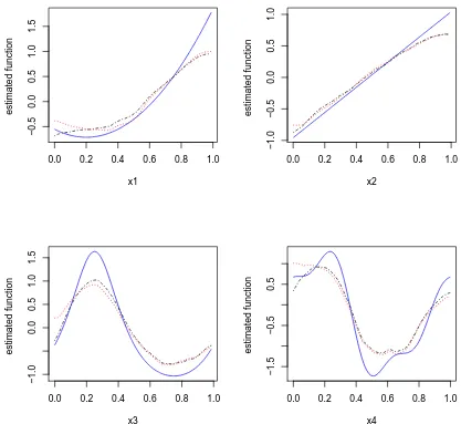
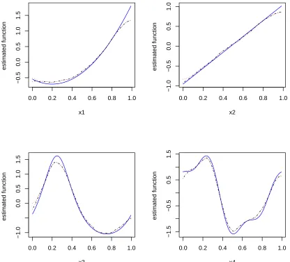
Figure 2.1 The estimated nonparametric functions averaged over 100 simula-tion runs with the MLE and REML type of methods for simulasimula-tion setting I: n = 200, w = 1. The blue solid lines are the true under-lying functions. The black dot-dashed lines are estimates using the MLE type of method. The red dotted lines are estimates using the REML type of method. . . 36 Figure 2.2 Empirical coverage probabilities of 95% pointwise confidence
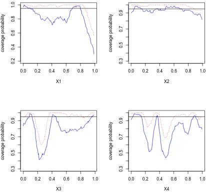
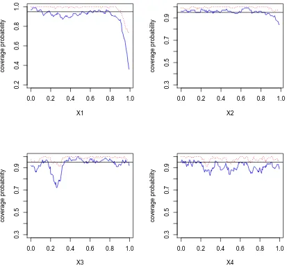
in-tervals with the MLE type of method for simulation setting I:
n = 200, w = 1. The blue solid lines are coverage probability based on frequentist estimation and the red dotted lines are cover-age probability based on Bayesian estimation. . . 37 Figure 2.3 Empirical coverage probabilities of 95% pointwise confidence
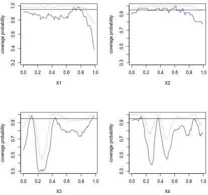
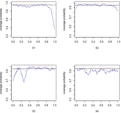
in-tervals with the REML type of method for simulation setting I:
n = 200, w = 1. The blue solid lines are coverage probability based on frequentist estimation and the red dotted lines are cover-age probability based on Bayesian estimation. . . 38 Figure 2.4 The estimated nonparametric functions averaged over 100
simula-tion runs with the MLE and REML type of methods for simulasimula-tion setting II:n= 200, w = 5. The blue solid lines are the true under-lying functions. The black dot-dashed lines are estimates using the MLE type of method. The red dotted lines are estimates using the REML type of method. . . 39 Figure 2.5 Empirical coverage probabilities of 95% pointwise confidence
in-tervals with the MLE type of method for simulation setting II:
n = 200, w = 5. The blue solid lines are coverage probability based on frequentist estimation and the red dotted lines are cover-age probability based on Bayesian estimation. . . 40 Figure 2.6 Empirical coverage probabilities of 95% pointwise confidence
in-tervals with the REML type of method for simulation setting II:
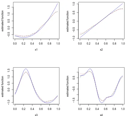
n = 200, w = 5. The blue solid lines are coverage probability based on frequentist estimation and the red dotted lines are cover-age probability based on Bayesian estimation. . . 41 Figure 2.7 The estimated nonparametric functions averaged over 100
Figure 2.8 Empirical coverage probabilities of 95% pointwise confidence in-tervals with the MLE type of method for simulation setting III:
n = 300, w = 1. The blue solid lines are coverage probability based on frequentist estimation and the red dotted lines are cover-age probability based on Bayesian estimation. . . 43 Figure 2.9 Empirical coverage probabilities of 95% pointwise confidence
in-tervals with the REML type of method for simulation setting III:
n = 300, w = 1. The blue solid lines are coverage probability based on frequentist estimation and the red dotted lines are cover-age probability based on Bayesian estimation. . . 44 Figure 2.10 The estimated nonparametric functions averaged over 100
simula-tion runs with the MLE and REML type of methods for simulasimula-tion setting IV: n = 300, w = 5. The blue solid lines are the true un-derlying functions. The black dot-dashed lines are estimates using the MLE type of method. The red dotted lines are estimates using the REML type of method. . . 45 Figure 2.11 Empirical coverage probabilities of 95% pointwise confidence
in-tervals with the MLE type of method for simulation setting IV:
n = 300, w = 5. The blue solid lines are coverage probability based on frequentist estimation and the red dotted lines are cover-age probability based on Bayesian estimation. . . 46 Figure 2.12 Empirical coverage probabilities of 95% pointwise confidence
in-tervals with the REML type of method for simulation setting IV:
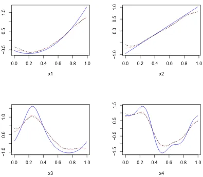
n = 300, w = 5. The blue solid lines are coverage probability based on frequentist estimation and the red dotted lines are cover-age probability based on Bayesian estimation. . . 47 Figure 2.13 The estimated nonparametric functions using the MLE and REML
type of methods for simulation setting V: n = 300, w = 1, β0 =
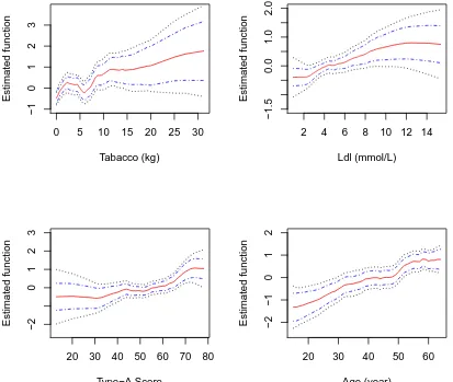
−3.5. The blue solid lines are the true underlying functions. The black dot-dashed lines are estimates using the MLE type of ap-proach. The red dotted lines are estimates using the REML type of approach. . . 48 Figure 2.14 The estimated functions corresponding to selected covariates in
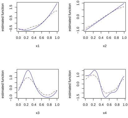
Figure 3.1 The estimated nonparametric functions averaged over 100 simu-lation runs with MLE and REML type of methods for simusimu-lation setting I: m = 75, w = 1 in model (3.16). The blue solid lines are the true underlying functions. The black dot-dashed lines are estimates using the MLE type of method. The red dotted lines are estimates using the REML type of method. . . 73 Figure 3.2 Empirical coverage probabilities of 95% pointwise confidence
in-tervals with the MLE type of method for simulation setting I:
m = 75, w = 1 in model (3.16). The blue solid lines are cover-age probability based on frequentist estimation and the red dotted lines are coverage probability based on Bayesian estimation. . . . 74 Figure 3.3 Empirical coverage probabilities of 95% pointwise confidence
in-tervals with the REML type of method for simulation setting I:
m = 75, w = 1 in model (3.16). The blue solid lines are coverage probability based on frequentist estimation and the red dotted lines are coverage probability based on Bayesian estimation. . . 75 Figure 3.4 The estimated nonparametric functions averaged over 100
simu-lation runs with MLE and REML type of methods for simusimu-lation setting II: m = 75, w = 5 in model (3.16). The blue solid lines are the true underlying functions. The black dot-dashed lines are estimates using the MLE type of method. The red dotted lines are estimates using the REML type of method. . . 76 Figure 3.5 Empirical coverage probabilities of 95% pointwise confidence
in-tervals with the MLE type of method for simulation setting II:
m = 75, w = 5 in model (3.16). The blue solid lines are coverage probability based on frequentist estimation and the red dotted lines are coverage probability based on Bayesian estimation. . . 77 Figure 3.6 Empirical coverage probabilities of 95% pointwise confidence
in-tervals with the REML type of method for simulation setting II:
m = 75, w = 5 in model (3.16). The blue solid lines are coverage probability based on frequentist estimation and the red dotted lines are coverage probability based on Bayesian estimation. . . 78 Figure 3.7 The estimated nonparametric functions averaged over 100
Figure 3.8 Empirical coverage probabilities of 95% pointwise confidence in-tervals with the MLE type of method for simulation setting III:
m= 100, w = 1 in model (3.16). The blue solid lines are coverage probability based on frequentist estimation and the red dotted lines are coverage probability based on Bayesian estimation. . . 80 Figure 3.9 Empirical coverage probabilities of 95% pointwise confidence
in-tervals with the REML type of method for simulation setting III:
m= 100, w = 1 in model (3.16). The blue solid lines are coverage probability based on frequentist estimation and the red dotted lines are coverage probability based on Bayesian estimation. . . 81 Figure 3.10 The estimated nonparametric functions averaged over 100
simu-lation runs with MLE and REML type of methods for simusimu-lation setting IV: m = 100, w = 5 in model (3.16). The blue solid lines are the true underlying functions. The black dot-dashed lines are estimates using the MLE type of method. The red dotted lines are estimates using the REML type of method. . . 82 Figure 3.11 Empirical coverage probabilities of 95% pointwise confidence
in-tervals with the MLE type of method for simulation setting IV:
m= 100, w = 5 in model (3.16). The blue solid lines are coverage probability based on frequentist estimation and the red dotted lines are coverage probability based on Bayesian estimation. . . 83 Figure 3.12 Empirical coverage probabilities of 95% pointwise confidence
in-tervals with the REML type of method for simulation setting IV:
m= 100, w = 5 in model (3.16). The blue solid lines are coverage probability based on frequentist estimation and the red dotted lines are coverage probability based on Bayesian estimation. . . 84 Figure 3.13 The estimated nonparametric functions averaged over 100
simu-lation runs with MLE and REML type of methods for simusimu-lation setting V: m = 100, w = 1, bi ∼ N(0,0.2), β0 = −5.5. The blue
solid lines are the true underlying functions. The black dot-dashed lines are estimates using the MLE type of method. The red dotted lines are estimates using the REML type of method. . . 85 Figure 3.14 The estimated functions corresponding to selected covariates in the
Figure 1 The estimated nonparametric functions averaged over 100 sim-ulation runs with the MLE and the REML type of methods for simulation setting VI: m = 75, w = 1 in model (3.18). The blue solid lines are the true underlying functions. The black dot-dashed lines are estimates using the MLE type of method. The red dotted lines are estimates using the REML type of method. . . 96 Figure 2 Empirical coverage probabilities of 95% pointwise confidence
in-tervals with the MLE type of method for simulation setting VI:
m = 75, w = 1 in model (3.18). The blue solid lines are coverage probability based on frequentist estimation and the red dotted lines are coverage probability based on Bayesian estimation. . . 97 Figure 3 Empirical coverage probabilities of 95% pointwise confidence
in-tervals with the REML type of method for simulation setting VI:
m = 75, w = 1 in model (3.18). The blue solid lines are coverage probability based on frequentist estimation and the red dotted lines are coverage probability based on Bayesian estimation. . . 98 Figure 4 The estimated nonparametric functions averaged over 100
sim-ulation runs with the MLE and the REML type of methods for simulation setting VII: m = 75, w = 5 in model (3.18). The blue solid lines are the true underlying functions. The black dot-dashed lines are estimates using the MLE type of method. The red dotted lines are estimates using the REML type of method. . . 99 Figure 5 Empirical coverage probabilities of 95% pointwise confidence
in-tervals with the MLE type of method for simulation setting VII:
m = 75, w = 5 in model (3.18). The blue solid lines are coverage probability based on frequentist estimation and the red dotted lines are coverage probability based on Bayesian estimation. . . 100 Figure 6 Empirical coverage probabilities of 95% pointwise confidence
in-tervals with the REML type of method for simulation setting VII:
m = 75, w = 5 in model (3.18). The blue solid lines are coverage probability based on frequentist estimation and the red dotted lines are coverage probability based on Bayesian estimation. . . 101 Figure 7 The estimated nonparametric functions averaged over 100
Figure 8 Empirical coverage probabilities of 95% pointwise confidence in-tervals with the MLE type of method for simulation setting VIII:
m= 100, w = 1 in model (3.18). The blue solid lines are coverage probability based on frequentist estimation and the red dotted lines are coverage probability based on Bayesian estimation. . . 103 Figure 9 Empirical coverage probabilities of 95% pointwise confidence
in-tervals with the REML type of method for simulation setting VIII:
m= 100, w = 1 in model (3.18). The blue solid lines are coverage probability based on frequentist estimation and the red dotted lines are coverage probability based on Bayesian estimation. . . 104 Figure 10 The estimated nonparametric functions averaged over 100
sim-ulation runs with the MLE and the REML type of methods for simulation setting IX: m = 100, w = 5 in model (3.18). The blue solid lines are the true underlying functions. The black dot-dashed lines are estimates using the MLE type of method. The red dotted lines are estimates using the REML type of method. . . 105 Figure 11 Empirical coverage probabilities of 95% pointwise confidence
in-tervals with the MLE type of method for simulation setting IX:
m= 100, w = 5 in model (3.18). The blue solid lines are coverage probability based on frequentist estimation and the red dotted lines are coverage probability based on Bayesian estimation. . . 106 Figure 12 Empirical coverage probabilities of 95% pointwise confidence
in-tervals with the REML type of method for simulation setting IX:
Chapter 1
Introduction
Modeling is fundamental in statistics research as it explains the relationship between the responses of interest and a number of predictor variables. But not all of the covariates truly make significant contributions to the response variable. The more covariates the model includes, the less estimate bias the prediction has. Yet, it will generate a large variance in prediction given too many covariates in the model. Besides, a model cannot be easily fit and does not have a meaningful interpretation with a bunch of uninformative variables. Thus, one of the crucial tasks is to identify the informative covariates in the model and eliminate the ones with rare contribution. With a relatively small number of important predictors, a model can have a parsimonious interpretation and the prediction will be more reliable.
1.1
Literature Review on Variable Selection
Meth-ods
1.1.1
Linear Regression Models and Variable Selection
Meth-ods
for-mulation of a linear regression model can be expressed as
yi =β1xi1+. . .+βpxip+ϵi, i= 1, . . . , n, (1.1)
where yi is the ith response, n is the number of observations, and ϵi is the error term,
usually assumed to be from normal distributionN(0, σ2). The linear relationship between the responses and the covariates is established by the coefficients β1, . . . , βp, and the
contribution of one covariate is fully reflected by the corresponding coefficient. As a result, a variable is informative if the corresponding coefficient estimate is significant from zero.
Many variable selection methods have been proposed for linear regression models. The traditional methods are discrete processes, such as the best subset search, forward selection, backward elimination, and stepwise selection. The descriptions of these meth-ods are presented below.
• Best subset search: We do an exhaustive search on all possible subsets of covari-ates and build models on each subset. The best model is selected according to a selection criterion. The commonly used criteria are Mallows’ Cp (Mallows, 1973),
AIC (Akaike, 1973) and BIC (Schwarz, 1978). Best subset search investigates all possible model compositions, which guarantees to obtain the best model given a selection criterion. However, it could be a very time-consuming or even infeasible procedure if the number of covariates is large.
• Forward selection: The model starts with an empty set, with no variables selected. Then we sequentially add one variable which improves the model fit most. The selection procedure will stop if no variable would increase the model fit significantly. Miller (1990) argued that forward selection works very well if the covariates are independent. But independence is a very strong assumption in practice.
• Stepwise selection: The procedure is a combination of forward selection and back-ward elimination and it allows either adding or dropping a variable in each step. Compared to forward selection and backward elimination, stepwise selection is more time-consuming and cannot deal with the collinearity case.
As discussed in the discrete processes, we either keep or drop a variable in the model at each step. They are intuitive and simple to implement, which makes them perform well in reality. But they are highly variable due to the discreteness (Breiman, 1996; Fan and Li, 2001). With a small perturbation in the data, selected variables could be dramatically different. Besides, it is hard to establish asymptotic theory and make inferences using these methods.
Accordingly, a family of shrinkage methods were proposed to address the issues. With a penalty term added to the residual sum of squares, we can estimate the linear coefficients by minimizing the penalized sum of squares. It is a continuous procedure and shrinks the coefficients with noninformative variables to zero while keeping the coefficients with a large magnitude for important variables. Those variables with negligible coefficients estimate are unimportant and therefore they should be eliminated from the model. Thus, the shrinkage methods are unified methods for model selection and estimation. They are more stable than the discrete processes and do not suffer from high variability. Besides, valid asymptotic inferences can be derived in these methods.
The spirit of the shrinkage methods is to minimize the objective function expressed as
L(β, y, x) +λJ(β), (1.2)
where L(β, y, x) is the loss function and λJ(β) is a shrinkage penalty term. For linear regression models in (1.1), the loss function is written as
L(β, y, x) =
n
∑
i=1
{yi−
p
∑
j=1
βjxij}2. (1.3)
Some popular methods with various penalty terms were proposed. The Lq shrinkage
family includes
• L0: penalty term is λ
∑p
j=1I(βj ̸= 0), proposed by Donoho and Johnstone (1988),
• L1 (LASSO): penalty term is λ
∑p
• L2 (Ridge): penalty term is λ
∑p j=1β
2
j, proposed by Hoerl and Kennard (1970a,
1970b),
• L∞ (Supnorm penalty): penalty term is λmaxj|βj|, proposed by Zhang et al.
(2008).
Other shrinkage methods are
• nonnegative garrote (Breiman, 1995). The estimates can be obtained by minimizing ∑
i(yi −
∑p
i=1ckβˆkxik)
2, with c
k ≥ 0,
∑
kck < s, where ˆβk is the ordinary least
square estimator ofβk.
• the SCAD (Fan and Li, 2001). The penalty function is written as follows
λ|β| if |β| ≤λ,
− |β|2−2aλβ+λ2
2(a−1) if λ < β ≤aλ, (a+ 1)λ2
2 if |β|> aλ,
where a >2 and λ >0 are tuning parameters.
• elastic net (Zou and Hastie, 2005). The penalty term is expressed as λ|βj|+ (1− λ)β2
j, λ∈[0,1].
Among the shrinkage methods, LASSO enjoys its popularity. Taking a linear regres-sion model of (1.1) as an example, the vector of coefficient estimate ˆβ∗ = ( ˆβ1∗,βˆ2∗, . . . ,βˆp∗)T can be solved with LASSO by minimizing the following objective function
n
∑
i=1
(yi− p
∑
j=1
βjxij)2+λ p
∑
j=1
|βj|, (1.4)
where λ is the shrinkage parameter, controlling the amount of shrinkage. A large λ
will generate a high shrinkage. LASSO shrinks both the informative coefficients and the noninformative coefficients with the same strength, which is not efficient in some cases.
Therefore, it is reasonable to select a group of variables instead of individual variables. Given a vector η ∈ Rd,(d ≥ 1) and a positive definite matrix K
d×d, we let ||η||K =
(ηTKη)12. Then, the estimate of the group LASSO can be achieved by minimizing the
following function
n
∑
i=1
(yi− p
∑
j=1
βjxij)2 +λ p
∑
j=1
||βj||Kj, (1.5)
where the positive λ is a tuning parameter.
Another generalization method is the adaptive LASSO, proposed by Zou (2006) and it was extended to Cox’s proportional hazards models by Zhang and Lu (2007). We apply the adaptive LASSO as the variable selection method in our study. Thus, we briefly introduce the adaptive LASSO below. The adaptive LASSO improves LASSO by applying different weights for different coefficients, imposing big effects on noninformative variables and small impacts on informative variables. Essentially, the objective function to be minimized is
n
∑
i=1
(yi − p
∑
j=1
βjxij)2+λ p
∑
j=1
ˆ
wj|βj|, (1.6)
where ˆwj is the weight associated with βj. The weight vector ˆw = ( ˆw1, . . . ,wˆp)T = |βˆ1|γ, whereγ >0, and ˆβ = ( ˆβ1, . . . ,βˆp)T is the ordinary least square estimator. Obviously,
big-ger weights are associated with smaller parameter estimates, which ensures more impacts on the less informative variables. Zou (2006) stated that the adaptive LASSO enjoys the oracle properties if the weights are data-driven and smartly selected. In addition, he argued that the formulation (1.6) is a convex function, which implies that the multiple local minima issue does not exist and we can achieve the global minimizer. Due to these advantages, the adaptive LASSO becomes a popular method in variable selection.
If we use maximum likelihood estimator ˆβ, the adaptive LASSO will obtain the coef-ficient estimates by maximizing the following penalized function
n
∑
i=1
ℓi(β1, . . . , βp;yi)−λ p
∑
j=1
ˆ
wj|βj|, (1.7)
where ℓi(β1, . . . , βp;yi) is the log-likelihood contributed byyi.
referred to Mitchell and Beauchamp (1988), Pereira and Stern (2001), Yuan and Lin (2005). One relatively new model selection method, called False Selection Rate (FSR) approach, was proposed by Wu, Boos and Stefanski (2007). They put a number of pseudo-variables to the real data set and perform model selection by controlling the FSR which is the proportion of noninformative variables selected in the models.
1.1.2
Nonparametric Models and Variable Selection Methods
Linear relationship between the response variable and the covariates is a strong assump-tion which is not necessarily valid for each model in practice. There are models where the linearity assumption does not hold. If we still fit such models by linear method, the prediction is misleading and model misspecification occurs. Under this circumstance, a nonparametric model would be more appropriate. Basically, a general nonparametric model takes the formyi =f(xi1, . . . , xip) +ϵi, i= 1, . . . , n, (1.8)
whereyiis theith observation,nis the number of observations, andf(.) is a non-specified
function. Usually, we assume f(.) to be smooth and continuous. If f(xi1, . . . , xip) = β1xi1 +. . .+βpxip, a nonparametric model becomes a linear regression model. In
non-parametric modeling, how to estimate the function f(.) plays a critical role. Kernel estimations, regression splines and smoothing splines are well-known estimation meth-ods.
Kernel estimation methods use linear estimators to predict the value at a particu-lar point x. One famous linear estimator is Nadaraya-Watson estimator which can be expressed as
ˆ
fh(x) =
∑n
i=1Kh(xi−x)yi
∑n
i=1Kh(xi−x)
, (1.9)
where K is a kernel function and h is a bandwidth which is a smoothing parameter controlling the size of the local neighborhood. Some commonly used kernel functions include the Gaussian kernel and the symmetric Beta family kernel.
Regression splines estimation is another way to estimate a nonparametric function with a set of basis functions as follows
ˆ
f(x) =b0+b1x1+. . .+brxr+ m
∑
j=1
whereris the order of the regression spline,kj is thejth knot,{b0, . . . , br, β1, . . . , βm}T is a
set of coefficients, and (a)+ isaifais greater than 0, and 0 otherwise. The representation
of the regression splines in (1.10) is a linear combination of two parts{xj}r
j=0, and {(x− kj)r+}mj=1. Some other popular basis functions are B-spline basis, natural splines, and
radial basis functions (Eilers and Marx, 1996; Green and Silverman, 1994). We use the smoothing splines to estimate the nonparametric functions, and hence we will explain it extensively in the following section.
One unavoidable drawback in nonparametric models is the “curse of dimensionality”. The variance of the estimates greatly inflates as the number of independent variables increases. To deal with the issue, Hastie and Tibshirani (1986) proposed additive regres-sion models. Denote by yi the ith observation out of n observation units (i = 1, . . . , n).
We can write an additive regression model as
yi =α+f1(xi1) +. . .+fp(xip) +ϵi, i= 1, . . . , n, (1.11)
where α is a constant, fj(.)’s (j = 1, . . . , p) are one-dimensional smooth and continuous functions, and ϵi is assumed to be distributed from a normal distribution.
There are two benefits of the additive models. Firstly, due to the fact that each additive term can be estimated individually, the curse of dimensionality is no longer a problem. Secondly, the additive relationship can clearly explain the contribution of each covariate to the response variable. Compared to the general nonparametric regression models in (1.8), the additive models have restricted applications because the nonparamet-ric functionf(.) in nonparametric regression is decomposed into several one-dimensional nonparametric functions in additive models. Whereas, the additive models are popular in the real applications due to their straightforward interpretation and model conciseness.
Another well-known model in the nonparametric framework is the smoothing spline analysis of variance (SS-ANOVA) which was proposed by Wahba (1990). The regression function in SS-ANOVA can be written as
f(x) =b+
p
∑
j=1
fj(xj) +
∑
1≤j<k≤p
fjk(xj, xk) +. . .+f1...p(x1, . . . , xp), (1.12)
If the interactions in (1.12) are eliminated, SS-ANOVA is reduced to an additive model. Variable selection becomes a challenge in nonparametric models. In context of lin-ear models, the importance of variables is completely reflected by their corresponding coefficients. A variable is considered as a noninformative one if its coefficient estimate is negligible. But it is not the case in the nonparametric framework. Since the nonparamet-ric functions are not specified, we can only drop a variable from the model if the function associated with that variable is estimated to be a constant as a whole component.
One of the regression-spline-based model selection methods is the adaptive group LASSO (Huang et al. 2010) and it is applied in additive models. It is an iterative process, combining the group LASSO with the adaptive LASSO. Taking advantage of the representation of regression spline estimator for the nonparametric components, the method performs variable selection by estimating and selecting the groups of coefficients. The selection procedure has two steps. In the first step, the group LASSO is utilized to get the initial estimates and decrease the dimension of the model. In the second step, we apply the adaptive group LASSO to pick up the final nonparametric functions.
Another regression-spline-based method was proposed by Friedman (1991). He pre-sented a multivariate adaptive regression splines (MARS) algorithm to do model selection for high-dimensional cases. With the help of a basis function set, MARS performs vari-able selection in two steps. The first step is a forward process, adding two basis functions each time until a large number of variables are selected. One basis functions is
Bm(x) = Km ∏
k=1
[skm(xv(k,m)−tkm)]q+, (1.13)
whereKm denotes the number of factors in themth basis function,skm takes two values
±1 indicating the truncation side, andv(k, m) labels the predictor variables. The model is usually overfit after the first step. The second step is a backward process, punning the model to fit the data better. It drops variables one by one, eliminating the least informative one at every step until it gets the best model.
is a regularization with the penalty as the sum of component norms. We assume a nonparametric regression model in the formulation of (1.8). Based on the SS-ANOVA framework, f can be estimated by minimizing the regularization
1
n n
∑
i=1
{yi−f(xi)}2+τn2J(f), with J(f) =
p
∑
α=1
||Pαf||, (1.14)
where τn is the smoothing parameter and f belongs to a reproducing kernel Hilbert
space (RKHS), associated with the SS-ANOVA in (1.12). Let F denote the RKHS, and
Pαf is the orthogonal projection of f onto Fα which is one of p orthogonal subspaces
of F. By imposing a penalty of sum of norms of the functional components, COSSO performs model selection in a continuous shrinkage process. However, COSSO tends to oversmooth the functions, which sometimes keeps it from having the oracle property in the nonparametric framework. Motivated by the adaptive LASSO, Storlie et al. (2009) proposed the adaptive COSSO (ACOSSO) which puts different impacts on the functional components. The corresponding regularization is
1
n n
∑
i=1
{yi−f(xi)}2+τn2J(f), with J(f) =
p
∑
α=1
wα||Pαf||, (1.15)
where wα’s are the weights. In this way, more important functional components are exposed to smaller penalty compared to less important ones. Thus, the informative variables can be quickly identified and we don’t lose much information on the estimation of important functions.
Another smoothing-spline-based model selection method is nonnegative garrote com-ponent selection (NGCS) (Yuan 2007). NGCS is a generalization of nonnegative garrote (Breiman 1995) and is applied in nonparametric setting of (1.12). It is a shrinkage method and the shrinkage factord= (d1(λ), . . . , dp(λ))T is obtained by minimizing the following
regularization 1 2 n ∑ i=1
(yi−zid)2+nλ p
∑
j=1 dj
subject to dj ≥0, j = 1, . . . , p,
. . . ,fˆinit
1,...,p(xi))T, and λ > 0 is a tuning parameter. The estimates of the functional
components are then given byd1(λ) ˆf1init(xi1), . . . , d1,...,p(λ) ˆf1init,...,p(xi). One initial estimate
of functional components is smoothing spline estimate which minimizes
n
∑
i=1
{yi−f(xi)}2+τ1J1(f1) +. . . ,+τpJp(fp) +. . .+τ1,...pJ1,...,p(f1,...,p), (1.16)
where τ’s are the tuning parameters and J’s are the squared norms in the functional component spaces. It can be shown that the shrinkage parameter is large if the functional component estimate is small, while the shrinkage parameter is small if the functional component estimate is large. In this way, noninformative functional components will shrink to zero very fast but informative components will keep in a large magnitude.
Ravikumar et al. (2009) proposed a new class of sparse additive models (SpAMs) which have the mixed features of the additive nonparametric regression and the sparse linear modeling. They presented a method of fitting SpAMs in high dimensional data. Based on the additive regression model’s framework in (1.11), there are constraints im-posed on the functional componentsfj’s in order to keep the smoothness of the functional components and the sparsity across components. Let Hj indicate the Hilbert space of
the function fj(.) such that E{fj(.)} = 0, and E{fj2(.)} < ∞. Let the inner product < fj, fj∗ >= E{fj(tj), fj∗(tj)}, and fj(.) = βjgj(.). The SpAMs need to minimize the
following objective function
minβ∈Rp,g
j∈HjE{y−
p
∑
j=1
βjgj(tj)}2
subject to
p
∑
j=1
|βj|< L,
E(gj) = 0, j = 1, . . . , p,
E(gj2) = 1, j = 1, . . . , p. (1.17) The constraint on βj’s makes the sparsity of β’s and therefore some of the functional components fj’s will go to zero.
the model can be expressed as
yi =α+ p
∑
j=1
fj(xij) +
∑
j>k
fjk(xij, xik) +ϵi, i= 1, . . . , n, (1.18)
where α is a constant, fj’s are main effects, and fjk’s are two-way interactions. The
previous method in SpAMs cannot be applied here since there is no interaction terms in SpAMs. In addition, COSSO cannot perform well in this case because it is not good at handling the high dimensional situation. Radchenko and James (2010) proposed a variable selection using adaptive nonlinear interaction structures in high dimensions (VANISH) in this case. A simple approach to estimate the nonparametric functions is to minimize the penalized least squares as
n
∑
i=1
{yi −f(xi)}2+λ(
p
∑
j=1
||fj||2+
p
∑
j=1 p
∑
k=j+1
||fjk||2). (1.19)
The method shrinks a lot of main effects and two-way interactions to zero. But it imposes the same shrinkage on all terms including main effects and interactions, which is not efficient. Thus, Radchenko and James (2010) proposed a convex penalty function that imposes a constraint and adjusts the shrinkage on the interactions based on the different conditions whether or not the main effects are included in the model. The corresponding penalized function is
n
∑
i=1
{yi−f(xi)}2 +λ1(
p
∑
j=1
||fj||2 +
p
∑
k:k̸=p
||fjk||2)
1 2 +λ2
p
∑
j=1 p
∑
k=j+1
||fjk||. (1.20)
It also can be shown thatλ1 is treated as the weight associated with the penalty of every
additional predictor added into the model, and λ2 is an extra penalty of the interaction
terms.
Yang (2004) and Xue (2009).
1.2
A Smoothing Spline Estimation of a
Nonpara-metric Function
We use smoothing splines to estimate the nonparametric functions. First of all, we briefly introduce the reproducing kernel Hilbert space (RKHS) and the smoothing spline estimator. A Hilbert space, H, is an inner product space. It is also complete and separable with respect to the norm/distance function defined by the inner product. For any f,g ∈ H and a∈R, < ., . > is defined as an inner product if and only if it satisfies the following three properties:
• < f, g >=< g, f >,
• < f +g, h >=< f, h >+< g, h >, and < af, g >=a < f, g >, • < f, f >≥0 and equal if and only if f = 0.
A linear functionalLis a mapping of an element in the linear space to a real number. One fundamental theorem in Hilbert space is the Riesz theorem. It claims that for every continuous linear functional L in a Hilbert space H, there exists a unique gL∈ H such
that L(f) =< gL, f > for ∀f ∈ H. If a Hilbert space H is a real valued function space,
we can define an evaluation function Lt(f) which maps f to f(t). Furthermore, if the
evaluation function is bounded, i.e., |L(f)| ≤ M||f||H for a constant M, H becomes a reproducing kernel Hilbert space (RKHS). Let’s take the following simple regression model for example
yi =f(ti) +ϵi, i= 1, . . . , n,
where n is the number of observations. Without loss of generality, we assume that the knots are distinct and ordered, 0 ≤ t1 < . . . < tn ≤ 1, and ϵi’s are independent and
identically distributed from normal distributionN(0, σ2). In addition, we assume thatf
is a smooth function in the space
Wh ={g(t)|g(t), g(1)(t), . . . , g(h−1)(t) absolutely continuous,
∫ 1
0
where g(j)(t) denotes the jth derivative of g(t). After an inner product is defined by
< f1, f2 >Wh=
h
∑
j=1
f1(j−1)(0)f2(j−1)(0) + ∫ 1
0
f1(h)(u)f2(h)(u)du,
the space Wh is proved to be a reproducing kernel Hilbert space. Moreover, Wh can be
decomposed into two subspaces H0 and H1 where H0 denotes the space with constant
functions and H1 is the complement of H0. We can get the estimate of the smooth
function f(.) with
argminf∈Wh1
n n
∑
i=1
{yi−f(ti)}2+λ||P1f||2Wh, (1.21)
where the positive λ is the smoothing parameter and P1(f) denotes the projection off
into space H1. It can be shown that the expression in (1.21) is equivalent to
argminf∈Wh1
n n
∑
i=1
{yi−f(ti)}2+λ
∫ 1
0
{f(h)(t)}2dt. (1.22)
Alternatively, if the likelihood is specified, we can get the smoothing spline estimate by maximizing the penalized log-likelihood
ℓ{β, f(.);y} − λ
2 ∫ 1
0
{f(h)(t)}2dt, (1.23)
where ℓ(.) is the log-likelihood. The smoothing spline estimators have several represen-tations. We adopt the representation presented by Kimeldorf and Wahba (1971). The representation of the hth-order smoothing spline estimator is written as
f(t) =
h
∑
j=1
δjϕj(t) + n
∑
i=1
aiRh(t, ti), (1.24)
whereϕj(t) = (jtj−−1)!1 , j = 1, . . . , h, consisting of the basis of polynomials of order (h−1), and δj’s are fixed coefficients. In addition, Rh(t, ti) can be calculated as
Rh(t, ti) = 1 [(h−1)!]2
∫ 1
0
where (t−u)+ = t −u if t ≥ u and 0 otherwise. With the above expression, we can
easily get Rh(tk, tl) for quadratic smoothing spline (h = 1) and cubic smoothing spline
(h= 2). When h= 1, R1(tk, tl) = min(tk, tl), and whenh= 2, R2(tk, tl) = (3tk2tl−t3k)/6
given tk < tl.
1.3
The Linear Mixed Model Representation
Let δ= (δ1, . . . , δh)T,a = (a1, . . . , an)T, and denote by f the vector of f(t) evaluated at
point ti. The representation in (1.24) has the following matrix form
f =T δ+ Σa, (1.26)
where T is an n × h matrix with the (k, l)th element as ϕl(tk), and Σ is a positive
definite matrix with the (k, l)th element asRh(tk, tl). Furthermore, it can be shown that
the penalty term λ2 ∫01{f(h)(t)}2dt= λ2aTΣa, which implies thata can be considered as a random effect from normal distribution N(0, τΣ−1), withτ =λ−1. Thus, τ is treated as
an induced variance component from the nonparametric functionf. We can see that the smoothing spline estimator in (1.26) has a linear mixed model representation. Therefore, many methods valid in a linear setting could also be adapted. Two points from the linear mixed model representation should be noticed. One is that the nonparametric function
f is an (h−1)th polynomial if and only if the induced variance component τ is zero. The other is that f is constant if and only if τ is zero givenh = 1.
1.4
The Framework of the Dissertation
Chapter 2
Model Selection and Estimation in
Generalized Additive Models
2.1
Introduction
Linear regression is widely used because it has a straightforward interpretation and can be easily fit. In linear regression models, we usually assume that the responses follow a normal distribution. However, there are lots of situations where the responses are instead from a distribution in the exponential family. Thus, linear regression models are extended to generalized linear models where a link function is needed to relate the response variable to the linear predictors.
The objective of this chapter is to propose a method to perform model selection and estimation for generalized additive models. Below is an outline of this chapter. In Section 2.2, a short description of GAMs is given and the generalized linear mixed model representation of GAMs is also presented. Furthermore, the eigenvalue-eigenvector decomposition approach is introduced to simplify the matrix calculation. The adaptive LASSO is applied and the EM algorithms are derived for GAMs in Section 2.3. In Section 2.4 and 2.5, simulation studies are conducted, followed by an application on a real data set. We conclude this chapter with a summary in Section 2.6.
2.2
Generalized Additive Models and the
Represen-tation
2.2.1
Generalized Additive Models
Denote by yi the ith response variable out of n observations (i= 1, . . . , n). Assume that yi’s are independently distributed from a distribution in the exponential family. Besides,
there areppossible covariates contributing to the response variable. The generic form of generalized additive models can be expressed as
g(µi) =β0+f1(xi1) +f2(xi2) +· · ·+fp(xip), i= 1, . . . n, (2.1)
where g(.) is a link function, µi = E(yi|xi1, . . . , xip), β0 is a constant, and n is the
number of observations. It is assumed that f1(.), . . . , fp(.) are unspecified smooth
2.2.2
Quasi-likelihood and the Generalized Linear Mixed Model
Representation
Let’s see how to generate quasi-likelihood for a distribution in the exponential family. Supposeyi’s are independent and identically distributed from a distribution in the
expo-nential family. The probability density function of yi can be written as
f(yi, θi) = exp{
yiθi−b(θi) ai(ϕ)
+c(yi, ϕ)}, (2.2)
where θi is the natural parameter, ϕ is the known or unknown scale parameter and ai(ϕ) = mϕi with the positivemi being a known weight. In this dissertation, we consider
the cases with a known ϕ. Thus, we can generate the quasi-likelihood as follows. It can be easily obtained that the mean and variance components are
µi =E(yi|xi) = b
′ (θi),
var(yi|xi) =ai(ϕ)b
′′ (θi).
Thus, mean and variance are related throughθ. If mean is indicated byµi, variance can be
specified as ai(ϕ)v(µi), wherev(µi) is called the variance function. The quasi-likelihood
can be expressed as
L= exp{
n
∑
i=1
∫ µi
yi
mi(yi−u)
ϕv(u) du}, (2.3)
If deviance di =−2∫µi
yi
mi(yi−u)
v(u) du, we can have
L= exp{− 1 2ϕ
n
∑
i=1
di(yi, µi)}. (2.4)
Therefore, we can construct the quasi-likelihood in generalized additive models.
There are a number of ways to estimate nonparametric functions. Here, we use the smoothing splines estimation. As for the model setting described in (2.1), there are p
one-dimensional nonparametric functions f1, . . . , fp. Denote by ℓ{β0, f1(.), . . . , fp(.);y}
log-quasi-likelihood is written as
ℓ{β0, f1(.), . . . , fp(.);y} − λ1
2 ∫ b1
a1
{f1(h)(x1)}2dx1−. . .− λp
2 ∫ bp
ap
{fp(h)(xp)}2dxp, (2.5)
whereλj’s (j = 1,. . ., p) are the smoothing parameters associated with the nonparametric
functions fj’s, controlling the smoothness of the functions and the goodness of fit of
the model, and (aj, bj) is the range for covariate Xj. As λj increases, the smoothing
splines tend to oversmooth. Thus, it is important to choose an appropriate value for the smoothing parameter. Given λj’s, if we maximize the penalized log-quasi-likelihood in
(2.5) with respect to the nonparametric functions, we will get smoothing spline estimators of orderh (Kimeldorf and Wahba, 1971; Wahba, 1990; Zhang and Lin, 2003). We adapt the representation of smoothing spline estimation proposed by Kimeldorf and Wahba (1971).
Take f1(.) for example. Let x1 = (x11, x21, . . . , xn1)T denote the vector of n knots.
Denote byx0
1the vector ofr1 ordered and different knots inx1. Without loss of generality,
assume 0 < x0
11 < x021 < . . . < x0r11 < 1. According to the formulation in (1.26), the
hth-order smoothing splines estimation of f1(x1) is
f1(x1) = N1(T1δ1+ Σ1a1), (2.6)
where N1 is an incidence matrix that maps the vector x01 to the original vector x1, T1 is
ar1×h matrix with the (k, l)th element asϕl1(x0k1), Σ1 is a positive definite matrix with
the (k, l)th element as Rh(x0k1, x0l1),δ1 = (δ11, . . . , δh1)T, and a1 = (a11, . . . , ar11)
T, which
is assumed to be a random effect from normal distribution N(0, τ1Σ−11). Notice that τ1
is the inverse of smoothing parameter λ1 and it can be considered as an extra variance
component induced from f1.
Denote by y the vector of observations, i.e., y = (y1, y2, . . . , yn)T. Applying the
smoothing splines estimator to each nonparametric function, GAMs can be written as
g(µ) = 1β0+N1T1δ1+. . .+NpTpδp +N1Σ1a1+. . .+NpΣpap, (2.7)
where 1 is a vector of ones, β0, δj’s (j = 1, . . . , p) are fixed effects, and aj’s are random
effects. One special case is the quadratic smoothing spline (h=1) estimator, where Tj’s
are reduced to vectors and δj’s are reduced to scalars. Since ϕ1j(x) = x
1−1
(j = 1, . . . , p) arerj×1 vectors of ones and thus NjTj is ann×1 vector of ones. In this
case, the corresponding expression of GAMs can be expressed as
g(µ) = 1β0+ 1δ1+. . .+ 1δp+N1Σ1a1+. . .+NpΣpap
= 1β+N1Σ1a1+. . .+NpΣpap, (2.8)
where β0, δj’s (j = 1, . . . , p) are combined into a single term β, and aj’s are random
effects with normal distribution N(0, τjΣ−j1). As shown in (2.8), generalized additive
models can be written in a generalized linear mixed model representation. If the two components are specified as
µai = E(yi|a),
var(yi|a) = ai(ϕ)v(µai) = ϕ miv(µ
a i).
The quasi-likelihood can be calculated as
L= exp{
n
∑
i=1
∫ µa i
yi
mi(yi−u)
ϕv(u) du}= exp{− 1 2ϕ
n
∑
i=1
di(yi, µai)}. (2.9)
2.2.3
Eigenvalue-Eigenvector Decomposition
As the number of distinct knots rj’s (j = 1, . . . , p) and the number of covariates p
get large, the matrices involved in the model representation become highly dimensional, which makes the calculations time-consuming. To tackle this problem, we propose the eigenvalue-eigenvector decomposition approach to speed up the calculation. Let’s look at
f1first. The positive definite matrix Σ1 can be decomposed by the eigenvalue-eigenvector
approach. Thus, Σ1 =
∑r1
i=1λieieTi , where λi is the ith eigenvalue of Σ1, ei is the
corresponding eigenvector, and r1 is the dimension of Σ1. For positive eigenvalues, we
have λ1 > λ2 > . . . > λr1 > 0. If we pick up the first q1 leading eigenvalues and the
corresponding eigenvectors, Σ1 can be approximated as
Σ1 ≈E1Λ1E1T, (2.10)
where Λ1 = diag{λ1, . . . , λq1}, and E is constructed by the corresponding
eigenvec-tors, i.e., E1 = [e1, . . . , eq1]. The number of q1 is determined by the proportion of
min{q1 :
∑q1
i=1λi/
∑r1
i=1λi ≥p0}. Letb1 follow normal distributionN(0, τ1Λ1). Based on
the approximation, we can approximate Σ1a1 byE1b1, since both of them follow normal
distributions with the same mean 0 and the approximately equal variance, which is shown by
var(Σ1a1) =τ1Σ1 ≈τ1 q1
∑
i=1
λieieTi = var(E1b1). (2.11)
Furthermore, we reparameterize the random effect vector b1 to c1 such that c1 is
distributed as normal distribution N(0, τ1Iq1×q1). In this way, we keep the vector c1
with the same variance structure τ1Iq1×q1, and hence the estimate of c1 is stable and
has the same order of magnitude. Denote by B1 the matrix associated with c1. Then, B1 = [λ
1/2
1 e1, . . . , λ
1/2
q1 eq1] since
var(B1c1) = τ1 q1
∑
i=1
λieieTi = var(E1b1). (2.12)
We apply the same strategy to each random effect aj, j = 1, . . . , p. The GAMs in (2.8)
can be approximated as
g(µ) = 1β+N1B1c1+. . .+NpBpcp. (2.13)
Now cj’s (j = 1, . . . , p) are random effects from normal distribution N(0, τjIqj×qj). We implement the algorithm over the above model representation.
2.3
The Adaptive LASSO for Generalized Additive
Models
2.3.1
Methodology
We use the quadratic (h = 1) smoothing spline estimation in model selection. Through the eigenvalue-eigenvector decomposition and reparameterization, the nonparametric func-tion fj(.) can be written as
whereδj is a constant and cj = (c1j, . . . , cqjj)
T follows normal distribution N(0, τ
jIqj×qj). If the variance component τj is 0, fj(x) is reduced to a constant vector 1δj. Thus,
it does not make any contribution to the model and the corresponding covariate Xj
should be eliminated from the model. As a result, the model selection is reduced to the variance components estimation and selection. If the variance estimate is zero, the corresponding variable is noninformative. On the other hand, the informative variables will have significant estimates of variance components. Inspired by Zou (2006), Zhang and Lu (2007), we propose the adaptive LASSO for GAMs. Let the parameter set
θ = (β, τ1, . . . , τp)T whereτ1, . . . , τpare induced variance components from nonparametric
functions. Letc= (cT1, . . . , cTp)T. Apparently, the random effectcis distributed as normal distribution N(0,Σc), with the variance-covariance matrix as
Σc =
τ1Iq1×q1 0 ...
... ...
0 ... 0 τpIqp×qp .
The parameter estimates can be achieved by maximizing the penalized log-quasi-likelihood
ℓp(θ, λ;y) = ℓ(θ;y)−nλ p
∑
j=1 τj
˜
τj +ϵ
, (2.15)
subject to τj ≥0, j = 1, . . . , p,
where ˜τj’s are the estimators under the log-quasi-likelihood ℓ(θ;y). Small value of ϵ
(0.001) is chosen to avoid the cases of zero denominators. In order to get the good performance of the proposed method, the selection of the tuning parameter λ is impor-tant. We use Bayesian information criteria (BIC) to choose the best value of the tuning parameter on a one-dimensional grid search. BIC can be calculated by
BIC =−2ℓ+tlog(n), (2.16)
function. Givenh= 1, the estimated value of centered functionfj(.) at the set of ordered
and distinct knots x0
j can be obtained by
ˆ
fj(x0j) =Bjˆcj− 1 rj
11TBjcjˆ, (2.17)
where ˆcj is obtained by maximizing ℓ(θ;y), and rj is the number of points in x0j. In
addition, the centered function fj will give the estimated value at any arbitrary data
point xij by
ˆ
fj(xij) = Nijfjˆ, (2.18)
where Nij is theith row of the incidence matrix Nj.
The variance components are nonnegative. The true value of the variance component for a noninformative function is zero, which is on the boundary area. Maximizing the penalized log-quasi-likelihood in (2.15) directly is not an easy job due to the boundary issue. Moreover, there is no guarantee that the estimates of variance components are positive. To deal with these issues, we can instead use the EM algorithm (Dempster, 1977).
2.3.2
The EM Algorithm
The EM algorithm is an iterative process bouncing between the E-stage and the M-stage. At the E-stage, a conditional expectation of log-quasi-likelihood is calculated. At the M-stage, we maximize the conditional expectation from the E-stage to get the parameter estimates. With the EM algorithm, the likelihood always increases during the parameter update. In addition, the procedure of the parameter update can be carried out separately for smaller subsets of the whole parameter set.
2.3.2.1 The MLE type of EM Algorithm
Denote by Q the conditional expectation of the log-quasi-likelihood function. Under the mixed model representation in (2.13), we consider the random effectc= (cT1, . . . , cTp)T as missing data, and θ= (β, τ1, . . . , τp)T. At step t, the Q function can be written as