18th International Conference on Structural Mechanics in Reactor Technology (SMiRT 18) Beijing, China, August 7-12, 2005 SMiRT18-B01-7
p
-VERSION DIRECT TIME INTEGRATION METHOD AND ADAPTIVE
PROCEDURE FOR STRUCTURE DYNAMIC ANALYSIS
Xiaoping
Zheng
Phone: +86-10-62796187
Fax: +86-10-62781824
E-mail: [email protected]
Guowen Tan
Phone: +86-10-62778962
Fax: +86-10-62781824
E-mail: [email protected]
Zhenhan Yao
Phone: 86-10-62772913
Fax: +86-10-62781824
E-mail: [email protected]
Dept. of Engineering Mechanics
Tsinghua Univ., Beijing 100084, China
ABSTRACT
A new hierarchical direct time integration method for structural dynamic analysis is developed by using Taylor series expansions in each time step. High accuracy results can be obtained by increasing the order of the Taylor series. Furthermore, the local error can be estimated by simply comparing the solutions obtained by the proposed method with the higher order solutions. This local estimate is then used to develop an adaptive order-control technique. Numerical examples are given to illustrate the performance of the present method and its adaptive procedure.
Keywords: dynamic analysis; hierarchical integration; error estimates; adaptive procedure
1. INTRODUCTION
In recent years, error estimation and adaptive techniques have been emphasized in research on computational mechanics. The ultimate goal is to make the numerical solutions reliable in an efficient and economical manner. For structural dynamic problems, discretization errors that contain both spatial and temporal discretization errors can not be avoided. But these errors can be reduced. For the spatial discretization error, many techniques [1-4] have already been presented, such as h-refinement, p-refinement, and a combination of h- and p-refinement. Some of them are being incorporated into commercially available finite element codes. However, adaptive techniques for temporal discretization errors are just beginning to emerge. Zienkiewicz et al.[5] and Zienkiewicz together with Shiomi[6] introduced a simple expression as an indicator of the local error. Zienkiewicz and Xie[7] proposed another local error estimator by comparing the Newmark solutions with the exact solutions expanded in the Taylor series. Zeng et al. [8] obtained the same result in a more simple and intuitive way. Wiberg and Li [9] developed a more precise error estimator that can evaluate both displacement errors and velocity errors. Choi and Chung [10] presented global and local error estimates for various time integration methods. All of these efforts seek to find a reasonable step size so that the temporal discretization error is within the prescribed tolerance, which can be classified as the h-version method in the time domain.
In this paper, a new hierarchical direct time integration method for structural dynamic analysis is proposed by using Taylor series expansion in each time step. Compared with conventional direct time integration methods,
Copyright © 2005 by SMiRT18
t
0)
such as the Newmark method and the Wilson method, the present method can be used to adjust the order of the Taylor series in each time step to obtain very accurate results. Therefore, the method can be classified as the
p-version method in the time domain. Furthermore, the local error can be estimated by simply comparing the solutions obtained by the proposed method with the higher order values. This local estimate can be used to develop an adaptive order-control technique.
2. HIERARCHICAL DIRECT TIME INTEGRATION METHOD
After spatial discretization, a structural dynamic system can be generally represented by the following ordinary differential equations
( )t + ( )t + ( )t = ( )
MU&& CU& KU F (1)
with the initial conditions
0 0
|t= = (0), |t= = (
U U U& U& (2)
where M, C and K are the mass, damping and stiffness matrices, respectively; ,UandUare the displacement, velocity and acceleration vectors, respectively; and F(t) is the external force vector.
U & &&
The system described by equations (1)-(2) is usually solved by direct time integration methods, such as the Newmark method and the Wilson method. This study proposes a new hierarchical direct time integration method.
Let us consider a time interval
[ ,
. When the displacement U(t) and the velocity at time t are known from the results of the previous step calculations, any arbitrary order derivative of the displacement at time t can be obtained by differentiating the system equation (1)]
t t
+ ∆
t
U&( )t( 2) 1 ( ) ( 1) ( )
( )
( )
( )
( )
0, 1,
k k k k
t
t
t
t
k
+
=
−
−
+−
=
U
M
F
CU
KU
L
(3)where the superscript ‘(k)’ denotes the k-order derivative with respect to time.
Assuming
τ
∈[ ,t t + ∆t], the displacement at time τ can be expressed as a Taylor series as follows( ) 1 1 ( ) ( ) ( )( ) ! k k t t k τ ∞ = = +
∑
−U U U τ t k
t
(4)
Therefore, if the displacement and the velocity at time t are known exactly, equation (4) gives the exact value in the domain
[ ,
t t
+ ∆
t
]
. The approximate solutions at timet
+ ∆
can be obtained by truncating the Taylor series and takingτ
= +
t
t
t
+ ∆
∆
in expression (4). If n-order accuracy is required, the displacement andvelocity at time
t
can be expressed as nU
n(
t
+
∆
t
)
=
U
( )
t
+
∑
1
U
( )k( ) (
t
∆
t
)
kk=1
k
!
(5)&
(
)
&
( )
( )( ) (
)
U
U
U
n
t
+
t
=
t
+
t
t
−
+
∑
∆
11
1∆
!
n
k k
k
t
k=1 (6)
( 2) 1 ( ) (
(
)
(
)
k k
n
t
t
t
t
n+
+ ∆ =
−+ ∆ −
U
M
F
Similarly, the other higher order derivatives of the displacement at time
t
+ ∆
can be obtained as1) ( )
(
)
(
)
0, 1,
k k
n
t
t
t
t
k
+
+ ∆ −
+ ∆
=
CU
KU
L
(7)The above process is repeated to obtain the numerical solution at every time step. Compared with conventional direct time integration methods, such as the Newmark method and the Wilson method, the present method can be used to adjust the order of the Taylor series in each time step to obtain high accuracy results.
3. ERROR ESTIMATE AND ADAPTIVE PROCEDURE
To control the time discretization error, a procedure must be developed to measure the error.
Again, consider a time interval
[ ,
t t
+ ∆
t
]
and assumeτ
∈
[ ,
t t
+ ∆
t
]
. For a solution of n-order accuracy, the temporal discretization error of displacement at time τ isE
n( )
τ
=
U
e( )
τ
−
U
n( )
τ
(8)where Ue( )τ denotes the exact displacement.
Copyright © 2005 by SMiRT18 Since the exact displacement Ue( )τ can not be obtained in most real problems, the exact displacement will
be replaced by a n+1 order expression
e
n( )
τ
≈
U
n( )
τ
−
U
n( )
τ
=
1
U
(n+1)( ) (
t
τ
−
t
)
n+1n
(
+
)!
+1
1
(9)A pointwise definition of error, such as given in equation (9), is generally difficult to use as a criterion for order control, so various normalized measures are normally adopted. In this study, the local error of displacement in the interval
[ ,
t t
+ ∆
t
]
is measured bye
=
1
∫
t+∆te
( )
τ
d
τ
=
1
(
∆
t
)
n+1U
(n+1)( )
t
(
)!
n t n
t
n
+
2
∆
2
L
(10)
where the norm has been employed. For an arbitrary vector x, its
L
2 norm is defined as⊥
=
x
x x
.In addition, an appropriate tolerance for the absolute error in expression (10) is also difficult to specify, so a relative error is proposed as
n
e
n
+
(
)!
max max
U
2
U
(11) max U
η
n n nt
t
=
=
+ +e
n(
)
( )
( )
U
∆
1 1In expression (11) the denominator is the maximum displacement norm recorded during the
computation.
In this paper, the relative error
η
n is used as the local indicator for adaptive order control which requires that the order number n is chosen such that the relative errorη
n in each time step is less than a prescribed toleranceε
so thatη ε
k〉
k
=
n
−
2 3
, ,
L
,
1
η
n≤
ε
(12)The sum of the local errors given by expression (11) will give a reasonably good estimate for the global error.
+
n
n
steps
U
max steps(
2
)!
(13)η
=
∑
η
=
∑
+ + n nt
t
( )(
)
( )
1
1 1U
∆
u
=
&
=
where the summation runs over all time steps. Note that the order number n in expression (13) changes with the time steps.
4. NUMERICAL EXAMPLES
Two single degree-of-freedom examples with exact analytical solutions are presented in this section. These examples will be used to show the performance of the hierarchical integration method and its adaptive procedure.
The SDOF dynamic system can be expressed by
0 0
( )
(0)
(0)
mu
cu
ku
f t
u
u
u
+
+
=
=
&&
&
&
(14)
The first example is taken from Zienkiewicz and Xie[ ]. The parameters are specified as: m = 1, c = 0.6, k =
1, f = 1, , the time step size
7
(0)
0, (0)
0
u
=
u
&
∆
t
=
1
and the relative error toleranceε
=
0 001
.
0
&
(0)
=
4
. The
parameters for the second example are specified as: m = 1, c = 0.6, k = 16.09, f = 0,
u
,u
, thetime step size and the relative error tolerance
(0)
=
∆
t
=
0 5
.
ε
=
0 001
.
.The displacement response histories of for these two examples are respectively shown in Figures 1 and 3, in which three kinds of solutions are compared. The uniform solution was calculated using same order for every
Copyright © 2005 by SMiRT18 time step. The results in Figures 1 and 3 illustrate that the adaptive hierarchical solution is more accurate than the uniform solution. It also should be noticed that quite small time steps are unnecessary in the present method.
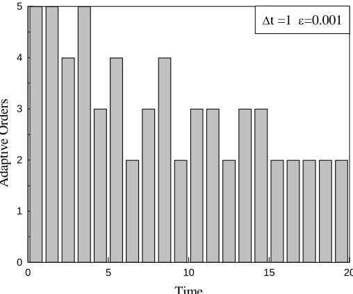
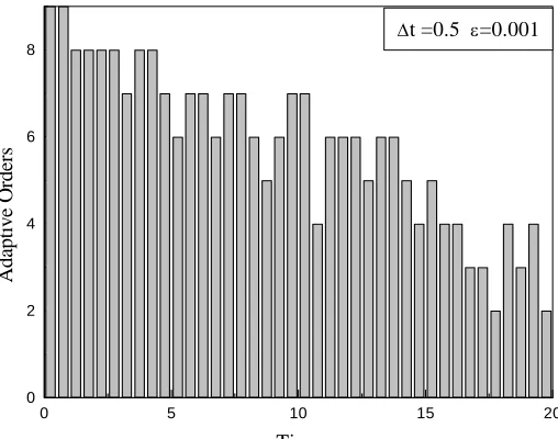
The variation of adaptive orders for different time steps are presented in Figures 2 and 4, which show that the abrupt change of displacement requires higher order. Moreover, since the damping has been considered in these examples, the order in the Taylor series has a decreasing tendency with time step forwarding.
0 5 10 15 20
0.0 0.5 1.0 1.5 2.0
Time
D
is
p
la
cem
ent
exact hierarchic uniform 3-order
Fig. 1 Displacement response history for example 1
0 5 10 15 20
0 1 2 3 4 5
∆t =1 ε=0.001
Time
Ada
p
ti
v
e Or
d
er
s
Fig. 2 Adaptive orders for example 1
Copyright © 2005 by SMiRT18
0 2 4 6 8
-1.0 -0.5 0.0 0.5 1.0
10
Time
D
isplacem
ent
exact hierarchic uniform 5-order
Fig. 3 Displacement response history for example 2
0 5 10 15 20
0 2 4 6 8
∆t =0.5 ε=0.001
Time
Ad
ap
ti
v
e O
rde
rs
Fig. 4 Adaptive orders for example 2
5. CONCLUSIONS
A new hierarchical direct time integration method is proposed for structural dynamic analysis, which uses Taylor series expansions in each time step. Compared with conventional direct time integration methods, such as the Newmark method and the Wilson method, the present method adjusts the order of the Taylor series in each time step to produce very accurate results. Therefore, the method can be classified as the p-version method in the time domain. Based on the local error estimate proposed in this study, an adaptive order-control technique is then developed. Numerical examples show that for a prescribed accuracy, the present method gives very accurate results in an economical and efficient way.
Copyright © 2005 by SMiRT18
REFERENCES
[1] Babuska I, Door M R. Error estimates for the combined h and p version of finite element method. Numer Math, 1981, 25:257-277
[2] Zienkiewicz O C, Gago J R, Kelly D W. The hierarchic concepts in finite element analysis. Comput & Struct, 1983, 16:53-65
[3] Babuska I, Zienkiewicz O C, Olivera E A, et al. Accuracy Estimates and Adaptivity for Finite Elements. John Wiley, New York, 1986
[4] Zienkiewicz O C, Zhu J Z. A simple error estimator and adaptive procedure for practical engineering analysis. Int J Numer Meth Eng, 1987, 24:337-357
[5] Zienkiewicz O C, Wood W L, Hine N W et al. A unified set of single algorithms. Part 1: General formulation and applications. Int J Numer Meth Eng, 1984, 20:1529-1552
[6] Zienkiewicz O C, Shiomi T. Dynamic behaviour of saturated porous media; The generalized Biot formulation and its numerical solution. Int J Numer Anal Meth Geomech, 1984, 8:71-96
[7] Zienkiewicz O C, Xie Y M. A simple error estimator and adaptive time stepping procedure for dynamic analysis. Earthquake Eng Struct Dyn, 1991, 8:871-887
[8] Zeng L F, Wiberg N E, Li X D, et al. A simple local error estimate and an adaptive time-stepping procedure for dynamic analysis. Earthquake Eng Struct Dyn, 1992, 21:555-571
[9] Wiberg N E, Li X D. A post-processing technique and an a posteriori error estimate for the Newmark method in dynamic analysis. Earthquake Eng Struct Dyn, 1993, 22:465-489
[10] Choi C K, Chung H J. Error estimates and adaptive time stepping for various direct time integration methods. Comput & Struct , 1996, 60:923-944