DOI: 10.1534/genetics.108.087361
The Polymorphism Frequency Spectrum of Finitely Many Sites
Under Selection
Michael M. Desai* and Joshua B. Plotkin
†,1*Lewis–Sigler Institute for Integrative Genomics, Princeton University, Princeton, New Jersey 08544 and†Department of Biology and Program in Applied Mathematics and Computation Science, University of Pennsylvania, Philadelphia, Pennsylvania 19104
Manuscript received January 21, 2008 Accepted for publication October 6, 2008
ABSTRACT
The distribution of genetic polymorphisms in a population contains information about evolutionary processes. The Poisson random field (PRF) model uses the polymorphism frequency spectrum to infer the mutation rate and the strength of directional selection. The PRF model relies on an infinite-sites approximation that is reasonable for most eukaryotic populations, but that becomes problematic whenuis large (u *0.05). Here, we show that at large mutation rates characteristic of microbes and viruses the infinite-sites approximation of the PRF model induces systematic biases that lead it to underestimate negative selection pressures and mutation rates and erroneously infer positive selection. We introduce two new methods that extend our ability to infer selection pressures and mutation rates at largeu: a finite-site modification of the PRF model and a new technique based on diffusion theory. Our methods can be used to infer not only a ‘‘weighted average’’ of selection pressures acting on a gene sequence, but also the distribution of selection pressures across sites. We evaluate the accuracy of our methods, as well that of the original PRF approach, by comparison with Wright–Fisher simulations.
M
UTATION rates and selective pressures are of central importance to evolution. The number and frequency distribution of genetic polymorphisms within a population carry information about these fundamental processes. Polymorphisms at higher fre-quencies reflect weaker selective pressures (or positive selection), and vice versa. Similarly, a larger number of polymorphisms indicates a higher mutation rate. Thus we can use the polymorphism frequency spectrum observed in genetic sequences sampled from a popula-tion to infer the mutapopula-tion rate and the selecpopula-tion pressure acting on the sequence.This intuition can be formalized into a rigorous method for estimating selection pressures and mutation rates by calculating the likelihood of sampled poly-morphism data as a function of these parameters. The Poisson random field (PRF) model provides an impor-tant and widely used method of doing so. The PRF model assumes a panmictic population of constant size, free recombination, infinite sites, no dominance or epistasis, and equal selection pressures at all sites. Under these assumptions, Sawyerand Hartl(1992)
showed that the distribution of frequencies of mutant lineages in a population forms a Poisson random field whose properties depend on the selection pressure and the mutation rate. Hartlet al.(1994) and Bustamante
et al.(2001) developed a maximum-likelihood method of estimating these parameters from data on the poly-morphism frequency spectrum. This method has been widely used to study, for example, purifying selection on synonymous (Hartlet al. 1994; Akashiand Schaeffer
1997; Akashi1999) and nonsynonymous (Hartlet al.
1994; Akashi1999) variation, and the evolution of base
composition (Lercheret al.2002; Galtieret al.2006).
Closely related to these analyses of polymorphism data are methods that calculate, on the basis of the PRF model, the ratio of the expected number of polymor-phisms within species to divergence between species for synonymous and nonsynonymous sites [using the idea behind the McDonald–Kreitman test (McDonaldand
Kreitman1991)]. These methods discard some of the
available data, as they depend only on the number of polymorphisms and not on their full frequency spec-trum. However, they are also less sensitive to assump-tions (Sawyer and Hartl 1992; Loewe et al. 2006).
Such methods have been applied to estimate selection pressures on synonymous variation (Akashi1995), on
nonsynonymous mutations in mitochondrial genomes (Nachman1998; Randand Kann1998; Weinreichand
Rand 2000), and on nonsynonymous variation in a
variety of nuclear genomes (Bustamante et al. 2002;
Sawyeret al.2003; Bartolomeet al.2005), including
humans (Bustamanteet al.2005).
Recent theoretical work has focused on relaxing various assumptions of the original PRF method. These include allowing for dominance (Williamson et al.
1Corresponding author:Department of Biology, University of
Pennsylva-nia, Philadelphia, PA 19104. E-mail: [email protected]
2004), population subdivision (Wakeley2003),
chang-ing population size (Williamson et al. 2005), and
linkage between sites (Zhu and Bustamante 2005).
Several methods for studying the properties of the dis-tribution of selection pressures across sites based on the PRF model have also been developed, using the poly-morphism frequency spectrum (Nielsen et al. 2005),
the ratio of polymorphism to divergence (Sawyeret al.
2003; Loeweet al.2006), or several of these methods in
conjunction (Bustamante et al. 2003; Piganeau and
Eyre-Walker2003; Boykoet al.2008).
A fundamental assumption of the PRF approach is that mutation is irreversible—the infinite-sites assump-tion. Thus any particular site can be only transiently polymorphic, and there is no steady-state solution to the evolutionary dynamics at any given site. However, since the constant creation of new polymorphic sites is bal-anced by older polymorphisms fixing or going extinct, the frequency distribution of polymorphisms across sites currently polymorphic does reach an equilibrium. This approach has important advantages. Since it describes the frequency spectrum of new mutations (‘‘derived alleles’’)—the frequency spectrum relative to the last ancestral state—it provides a natural framework for analyzing polymorphism data when the ancestral state is known. This ancestral state can often be inferred from an appropriate outgroup.
Despite its advantages, the infinite-sites approxima-tion can present problems. The approximaapproxima-tion is reasonable for most data currently available from typical eukaryotic populations. However, in many biologically reasonable parameter regimes, particularly those rele-vant to bacterial and viral populations, more than one mutational event may contribute to polymorphism at a given site. In this article, we show that under these parameter regimes the infinite-sites assumption causes the PRF method to underestimate negative selection pressures and mutation rates by as much as an order of magnitude. In addition, the PRF method often infers that a gene is under strong positive selection when in fact the gene is experiencing weak negative selection. This problem arises both for inferences based on the poly-morphism frequency spectrum and for inferences based on the ratio of within-species polymorphism to between-species divergence, but here we focus exclusively on the former.
In this article, we present two methods that relax the infinite-sites assumption of the PRF method, each with its own advantages and drawbacks. Rather than studying mutant lineages across a sequence, our methods focus on explicit models of the evolutionary dynamics at individual sites. We first present a modification of the PRF method that retains the essential framework, but calculates the frequency distribution of mutant lineages at each site rather than across the whole sequence. We next present an alternative method based on well-known diffusion equations in place of the PRF
frame-work. This alternative framework avoids all of the finite-site biases of the PRF, but it cannot make use of knowledge about the ancestral state. Rather than de-scribing a steady-state frequency distribution of derived nucleotides relative to this ancestral state, it describes the frequency distribution of all four nucleotides possible at each site—a fundamentally different steady state. Both of our methods allow us to estimate the selection pressure and the mutation rate from data on the polymorphism frequency spectrum. In addition, these methods also allow us to infer the distribution of selection pressures across sites.
To assess the accuracy of these methods, we generate polymorphism data from simulated Wright–Fisher pop-ulations with known selection pressures and mutation rates. By comparing inferences drawn from these simu-lated data sets, we demonstrate that our methods extend and improve upon the original PRF approach. Through-out this article, we focus on accurately inferring the sign and strength of negative selection, since the most trou-bling bias in the original PRF method is erroneous inference of positive selection when mutation rates are large. We focus primarily on situations when the ancestral state at each site cannot be reliably inferred, which is the typical situation when the mutation rate is large.
We emphasize that the effects of finite sites are of practical relevance only when the mutation rate is relatively large (u per site $0.05). As a result, the methods of inference developed here are not necessary for analyzing human or Drosophila population-genetic data. However, as we shall demonstrate, finite-site effects have significant practical implications when studying the population genetics of viruses, microbes, and some higher eukaryotes, such as sea squirts and starfish, that experience large mutation rates (Drake et al. 1998;
Lynchand Conery2003).
THEORY
The Poisson random field model of polymorphisms: We begin by outlining the PRF model of the site-frequency spectrum developed by Sawyer and Hartl (Sawyer and Hartl 1992; Hartl et al. 1994). This
model assumes that mutations occur in a population of effective sizeNat a Poisson rateNu, whereuis the per-sequencemutation rate, and are all subject to selection of strengths. The fate of each mutant lineage is modeled by a diffusion approximation to the processes of selection and drift. When a new mutant lineage enters the popu-lation, it is assumed to arise at a site that has not previously experienced any mutations (the infinite-sites assumption). Each mutant lineage is assumed to be independent of all others (the free-recombination assumption).
Extending earlier work by Wright (1938) and
a steady-state distribution of mutant lineage frequen-cies. They found that the number of lineages with frequency betweenxandx1dxis Poisson distributed with meanf(x)dx, where
fðxÞ ¼ul
1e2gð1xÞ 1e2g
1
xð1xÞ: ð1Þ
Hereg[Nsis a measure of the strength of selection on the mutant lineages andul[2Nuis twice the population
per-sequence mutation rate. The function f(x) is re-ferred to as a Poisson random field. In other words, the number of mutant lineages with frequency betweenx1 and x2 is a Poisson random variable with mean
Ðx2
x1 fðxÞdx. In addition, the number of mutant lineages with frequency in [x1,x2] is independent (as a random variable) from the number of mutant lineages with frequency in [y1, y2], provided these intervals do not intersect. Note thatf(x) is not integrable atx¼0. This divergence occurs because the steady state arises from a balance between new mutations constantly occurring and older lineages fixing or going extinct. Thus there is no finite, steady-state expression for the number of lineages that have fixed or gone extinct.
Hartl et al. (1994) and Bustamante et al. (2001)
used Equation 1 as the basis for maximum-likelihood (ML) estimation of the mutation rateuland selection pressure g from polymorphism data. They imagined sampling n individuals from a population with this steady-state distribution of segregating mutant lineages. They made the infinite-sites assumption that all mutant lineages occur at different sites, consistent with the earlier assumption that each lineage is independent. Since the number of mutant lineages at frequencyxin the population is Poisson distributed with meanf(x)dx, the number of sampled sites containing i mutant nucleotides (we refer to these asi-fold mutant sites) is Poisson distributed with mean
FðiÞ ¼ul
ð1
0
1e2gð1xÞ 1e2g
1 xð1xÞ
n
i x
ið1xÞni dx:
ð2Þ
This equation leads immediately to a maximum-like-lihood procedure for estimatinggandul(Bustamante
et al. 2001). A set of sequences from n sampled
individuals within a population will contain some number,yi, ofi-fold mutant sites for 0,i,n. The set
of values y1, y2,. . ., yn1 is called the site-frequency spectrum of the observed data. The probability of a spectrum {yi}, givengandul, is
Luðul;gÞ ¼
Y
n1
i¼1
eFði;g;ulÞ½Fði;g;ulÞ
yi yi!
: ð3Þ
For an observed spectrum {yi} in a particular data set,
one maximizes this likelihood overulandgto estimate the mutation rate and selection pressure.
The likelihood expression above assumes we know which nucleotide is ancestral and which nucleotide is the mutant (‘‘derived’’) at each polymorphic site. We refer to this situation as the unfolded case. When we do not have this information, we cannot distinguish be-tween ani-fold mutant site and an (ni)-fold mutant site. In this case, a data set will contain some number,yi,
i-fold and/or (n i)-fold mutant sites, where i runs between 1 and the largest integer#n/2. We refer to this as the folded case. In this situation, the likelihood of a particular data set Lfðul;gÞ is given by the same
expression as forLu, but with the product running from 1 ton/2 and withF(i) replaced byF(i)1F(ni) (except ifi¼n/2).
The infinite-sites approximation: The PRF model
makes two key assumptions: that each site is indepen-dent of all the others and that two mutant lineages never segregate at the same site. The former assumption is equivalent to assuming free recombination between all segregrating sites, and it has been investigated elsewhere (Akashiand Schaeffer1997; Bustamanteet al.2001);
we return to it in thediscussion. The main focus of this
article, however, is on the second assumption of the PRF, that there are an infinite number of sites, which has not been discussed much in the literature. This assumption can lead to problems that are most apparent when considering how the PRF method treats ‘‘multiply poly-morphic’’ sites—those that exhibit more than two types of segregating nucleotides. Polymorphisms of this type are indeed observed in data analyzed by the PRF method (Hartlet al.1994). We refer to the configuration of a
particular site as (a,b,c,d), wherea,b,c, anddare the numbers of sampled sequences that exhibit each of the four nucleotides. When we have unfolded data,ais the frequency of the ancestral nucleotide andb,c, andd are the frequencies of the three possible mutant nucle-otides, in order of decreasing frequency. For folded data,a,b,c, anddare the frequencies of all four possible nucleotides, again in order of decreasing frequency. In the original PRF analysis, a site with a (12, 1, 1, 0) configuration, for example, is treated identically to a site with a (12, 2, 0, 0) configuration. Such a treatment is incorrect: the former configuration can arise only from two mutant lineages, whereas the latter configuration could be caused by a single mutant lineage (presumably at relatively high frequency in the population). Yet the PRF analysis excludes the first possibility and treats both configurations as if they were (12, 2, 0, 0) sites (Hartl
et al.1994; Bustamanteet al.2001). Similarly, the PRF
method treats (10, 2, 2, 0), (10, 3, 1, 0), and (10, 2, 1, 1) sites as if they were in a (10, 4, 0, 0) configuration, etc.
same nucleotide. In other words, a (12, 2, 0, 0) site could reflect two low-frequency mutant lineages or one higher-frequency lineage, but the PRF method incor-rectly assumes that only the latter is possible. This leads to systematic biases in the estimates of selection and mutation obtained by the PRF method: by disregarding the possibility that an apparently high-frequency mu-tant lineage is actually several lower-frequency mumu-tant lineages, the PRF method underestimates the mutation rateuand the strength of negative selectionjsj.
Since a mutant lineage will survive on average Oðln½1=jsjÞgenerations before fixing or going extinct (Desai and Fisher 2007), and mutations arise at rate
Nmper site, the infinite-sites approximation will be valid only when Nmln½1=jsj>1 (although for sufficiently small samples the condition is weaker, since we may never sample multiple lineages even though they are segregating at the same site). This condition is some-times violated in real populations, particularly of viruses and microbes (e.g., Hartlet al.1994).
We stress that in parameter regimes relevant to most eukaryotes, including humans and Drosophila, finite-sites biases are negligible. But in parameter regimes relevant to bacteria and viruses, sites with multiple segregrating mutations have a disproportionate weight in estimates of selection and mutation, and thus they can lead to errors of an order of magnitude or more (Figure 1). In such circumstances, the PRF method also erroneously infers positive selection in many situations where selection is actually negative (Figure 1).
A per-site Poisson random field model of
poly-morphisms:In this section, we describe a method that
extends the PRF framework to the case of finite sites and takes full advantage of the information provided by the frequencies of all possible configurations at a site. The basic idea behind this modified approach is to recast the PRF framework on aper-sitebasis. We describe the steady-state frequency distribution of mutant lineages at a given site. From this, we can calculate the probability that a sample ofnindividuals will contain any configuration of mutants at that site. As in the original PRF method, we retain the assumption of free recombination, so that the DNA sequence is a collection of independent sites. Thus our per-site analysis leads directly to ML estimation of mutation rate and selection strength.
We begin by recasting the PRF expression for the steady-state distribution of mutant lineages to describe the frequencies of mutant lineages at a single site. At a given site, we have
fðxÞ ¼us1e
2gð1xÞ
1e2g 1
xð1xÞ; ð4Þ
whereusis theper-sitevalue,us¼2Nm, wheremis the per-site mutation rate. Using this formula to describe multiple lineages at a single site is somewhat peculiar, because this result assumes that all mutant lineages
behave independently of one another. Clearly this is not strictly true, since the mutant lineages are segregating at the same site. However, provided two mutant lineages rarely achieve simultaneous high frequencies in the population, then the assumption of independent mu-tant lineages is a good approximation. This assumption of noninteracting mutant lineages will often hold even when the other aspects of the infinite-sites approxima-tion are violated.
Analogous to the original PRF method, ata single site the number of mutant lineages that are observeditimes in a sample ofnsequences (‘‘i-fold mutant lineages’’) is Poisson distributed with mean
FðiÞ ¼us
ð1
0
1e2gð1xÞ 1e2g
1 xð1xÞ
n
i x
ið1xÞni dx:
ð5Þ
On the basis of this, we can calculate the probability of any particular polymorphism configuration at a site.
We begin by describing this calculation in the un-folded case. The probability that a site is monomorphic is just the probability that noi-fold mutant lineages are found at that site, for allibetween 1 andn1. This is
Pmono¼Pðn;0;0;0Þ¼eFð1ÞeFð2Þ . . . eFðn1Þ: ð6Þ
We define M [ Pmono to denote this monomorphism probability. The probability that a site exhibits a (n1, 1, 0, 0) configuration is the probability that a single 1-fold mutant lineage is sampled, and no 2-1-fold or higher lineages are found,
Pðn1;1;0;0Þ¼Fð1ÞM; ð7Þ
whereMdenotes the probability of monomorphism as above. The probability that a site exhibits an (n2, 2, 0, 0) configuration is more complex. This configuration could arise from a single 2-fold sampled lineage (as assumed under the standard PRF method) orit could arise from two 1-fold sampled mutant lineages that happen to involve mutations to the same nucleotide. Hence its probability is
Pðn2;2;0;0Þ¼ Fð1Þ2
2! M
1
31Fð2ÞM; ð8Þ
where the factor of 1
3 is the probability that two
mutations result in the same nucleotide. This expres-sion assumes that mutations between all possible nu-cleotides are equally likely—the obvious generalization applies when there are mutational biases, which we do not discuss further. Similarly the probability of an (n2, 1, 1, 0) configuration is
Pðn2;1;1;0Þ¼ Fð1Þ2
2! M
2
3: ð9Þ
an (n 4, 4, 0, 0) configuration, for example, is the probability of four 1-fold lineages to the same nucleo-tide plus the probability of two 1-fold lineages and a 2-fold lineage, plus the probability of two 2-2-fold lineages, plus the probability of one 1-fold lineage and one 3-fold lineage, plus the probability of a single 4-fold lineage. We have
Pðn4;4;0;0Þ¼M Fð1Þ4
4!
1 33 1
Fð1Þ2Fð2Þ
2!
1 32 1
Fð2Þ2
2!
1 3
1Fð1ÞFð3Þ1
31Fð4Þ
: ð10Þ
In general, the probability of a particular configuration is given by the sum of the probabilities of all possible partitions ofnthat lead to that configuration.
In the folded case, these calculations become fairly complex. The probability of a (12, 2, 0, 0) folded configuration, for example, includes the probability of a single 12-fold sampled lineage, as well as two 6-fold sampled lineages, and so on. Thousands of terms may arise in the expression for the probability of a particular configuration, even for moderate values ofn. We do not quote any of these expressions here, but rather we have developed a computer program to output symbolic ex-pressions for the probabilities of all possible folded as well as unfolded configurations, for a given sample size n. The algorithm used in this program is described in the
appendix, and the program is freely available on
request.
These probabilities of site configurations form the basis of maximum-likelihood parameter estimation. The probability of a data set withLtotal sites, including ya,b,c,dsites in configuration (a,b,c,d), is given by
L!
Q
ya;b;c;d!
Y
Pya;b;c;d
a;b;c;d; ð11Þ
where the products are over all possible configurations. Given a particular data set, we maximize this probability over us and g to find the ML estimate of these parameters. In the original PRF method, this maximi-zation is particularly simple, because the ML estimate foru can be expressed analytically in terms of the ML estimate for g, leaving a one-dimensional numerical maximization procedure to estimateg. In our per-site PRF method, however, a full two-dimensional numerical maximization is required to find the ML estimates ofus
andg. We have implemented a computer program to
perform this maximization; it is freely available on request.
Our per-site PRF method relaxes most of the con-sequences of the infinite-sites approximation inherent in the original PRF estimation procedure. We allow for the possibility that multiple mutant lineages contribute to the polymorphism observed at a single site. Thus we avoid the systematic underestimation of u and g, and incorrect inference of positive selection, that affect the
traditional PRF when mutation rates are large (Figure 1). This new method also uses all of the data available in the sample, including the differences between (n2, 2, 0, 0) and (n 2, 1, 1, 0) sites and the number of monomorphic sites (note the infinite-sites approxima-tion means that the original PRF cannot predict the number of monomorphic sites and hence makes no use of these data). It does still retain one aspect of the infinite-sites approximation: it assumes that mutant lineages segregating at the same site do not interfere with each other. This is never strictly true, but it is a good approximation unless multiple mutant lineages reach high frequency at a given site at the same time. Note that because of this assumption, the probabilities of all possible configurations (a,b,c,d) described above do not precisely sum to unity, because our approach allows a typically small but nonzero probability of multiple mutant processes adding to more than n sampled individuals. The no-interference assumption is substan-tially weaker than the infinite-sites assumption, and thus our revised sampling method extends the applicability of the PRF framework.
A per-site diffusion model of polymorphisms:In this
section, we describe a method that shifts fundamentally from the PRF framework and avoids all of the problems associated with the infinite-sites assumption. Rather than studying the distribution of the frequencies of mu-tant lineages, we focus on the evolutionary dynamics at each individual site, without keeping track of individual mutant lineages. We develop this into a maximum-like-lihood estimation ofgandufrom polymorphism data, which requires neither the infinite-sites nor the no-interference approximation described above. As in the original PRF method, we assume free recombination between sites.
At an individual site, we imagine that one nucleotide is preferred and the other three have the same fitness disadvantages(s,0). We assume that mutations occur at ratemand hence at ratem/3 between any two specific nucleotides (i.e., no mutational biases). These assump-tions simplify the discussion, but are not essential. In fact, one advantage of this approach is that these as-sumptions can be easily relaxed with obvious general-izations (noted below).
preferred nucleotidevs. the sum of the frequencies of the disfavored ones; this treatment is essentially a steady-state version of Williamsonet al.(2005). This simplified
model is not likely to be particularly useful, because it requires us to knowa priorithe identity of the preferred nucleotide, which in practice is part of what we wish to infer. This simplification also discards some of the information in the data [e.g., not making use of the difference between (12, 1, 1, 0) and (12, 2, 0, 0) sites]. However, first studying this analytically and computa-tionally simpler model makes the analysis of the full model more clear. We therefore begin by describing the one-dimensional method and then turn to the three-dimensional method.
The one-dimensional diffusion model: We begin by
describing a simplified diffusion approach that calcu-lates the frequency distribution of favoredvs.disfavored nucleotides, similar in spirit to that introduced by Mustonenand Lassig(2007). As noted above, we for
simplicity assume that one nucleotide is preferred and the other three nucleotides are disfavored. We denote the sum of the frequencies of the three disfavored alleles byx; the frequency of the preferred nucleotide is 1x.
We assume that mutation, selection, and random drift occur at each site according to standard Wright–Fisher dynamics. Thus the probability distribution ofxcan be described by the diffusion equation
@
@tfðx;tÞ ¼ 1 2
@2
@x2½vðxÞfðx;tÞ @
@x½mðxÞfðx;tÞ; ð12Þ
where f(x, t) is the probability that the disfavored nucleotides have frequencyx at time t and m(x) and v(x) are given by
mðxÞ ¼sxð1xÞ1mð1xÞ m
3x ð13Þ
vðxÞ ¼xð1xÞ
N ; ð14Þ
wheresis the selection coefficient against the disfavored nucleotides (s,0) andmis the per-site mutation rate per individual per generation. This diffusion equation is well known (Ewens 2004) and has the steady-state
solution derived by a zero-flux boundary condition:
fðxÞ ¼Cxus1ð1xÞus=31e2gx: ð15Þ HereCis a (us- andg-dependent) normalization factor, and as beforeus[2Nmandg[Ns.
If the frequency of disfavored nucleotides at a site equalsx, the probability that we findisuch nucleotides in a sample ofnindividuals isðn
iÞxið1xÞ ni
. Averaging overx, the overall probability that we sampleidisfavored nucleotides at a given site is
FðiÞ ¼ n i
ð1
0
Cxus1i1ð1xÞus=31ni1e2gxdx: ð16Þ
This integral, including the calculation of the normal-ization factorC, can be solved analytically. We find
FðiÞ
¼ n
i
Gðni1us=3ÞGði1usÞ1F1ði1us;n14us=3;2gÞ
Gðus=3ÞGðusÞ1F1ðus;4us=3;2gÞ
;
ð17Þ
whereGis Euler’s Gamma function and1F1is a hyper-geometric function.
The expression above leads immediately to a maxi-mum-likelihood method for estimatinggandusin the unfolded case. Note, however, that in contrast to the original PRF method, this model describes a steady state of the frequency distribution of preferred relative to unpreferred nucleotides, rather than derivedvs. ances-tral nucleotides. This is a very different sort of steady state, a point to which we return in more detail below. Since this model refers only to the preferred and unpreferred states at each site, it makes sense to apply to unfolded data only if we assume that the ancestral state is preferred. In a sample ofn sequences each of length L, we count the number of sites at which i disfavored nucleotides are sampled,yi, for 0 # i# n.
Since all sites are assumed independent, each with the polymorphism frequency distribution described above, the likelihood of the data given the parameters is
Luðus;gÞ ¼
L!
Qn i¼0yi!
Yn
i¼0
FðiÞyi: ð18Þ
nucleotide is the preferred one (Hartlet al.1994) is a
reasonable approach. But this approach will be in-accurate for sites where the most common nucleotide is not overwhelmingly so; when this situation describes a substantial fraction of sites, the method will fail. As a result, the one-dimensional diffusion framework does not allow for a rigorous ML estimate of parameters with folded data.
To perform rigorous ML fits to folded frequency data we must turn to a three-dimensional diffusion method.
The three-dimensional diffusion model:Rather than
considering all disfavored nucleotides as a single class, we can instead keep track of the evolutionary dynamics of all four possible nucleotides at a site. To do so, we assume the standard four-allele Wright–Fisher dynam-ics, with mutation at ratem=3 between any two particular nucleotides, and selection acting with strengthsagainst the three disfavored nucleotides. The dynamics can then be described by a three-dimensional diffusion equation for the joint distribution of the frequencies of the three disfavored allelesx1,x2, andx3,f(x1,x2,x3,t) (where the preferred allele has frequencyx0¼1x1
x2x3). We have
@
@tfðx1;x2;x3;tÞ
¼1
2
X3
i¼1
X3
j¼1
@2
@xi@xj Vij3f
X
3
i¼1
@ @xi
Mi3f
½ ; ð19Þ
where
Mi¼ ð11sÞxi 1
X3
j¼1
xj
!
1mð14xiÞ
3 ð20Þ
Vii ¼
xið1xiÞ
N ð21Þ
Vij ¼ xixj
N ; ði 6¼jÞ: ð22Þ
This is a somewhat less well-known diffusion equation (Wright 1949; Watterson 1977); the steady-state
solution is
fðx1;x2;x3Þ ¼C½x1x2x3ð1x1x2x3Þze2gðx11x21x3Þ; ð23Þ
whereCis a normalization factor, and we have defined z¼us/31.
Given the frequenciesx0,x1,x2, andx3of nucleotides in the population, the probability of sampling a site in anunorderedconfiguration (n0,n1,n2,n3) in a sample of
n individuals (adopting the convention that the first nucleotide listed is the preferred one) is just the multinomial probability
n!
n0!n1!n2!n3!
ð1x1x2x3Þn0x1n1x2n2x3n3: ð24Þ
Averaging overf, we therefore find that the probability of sampling a site in an unordered (n0, n1, n2, n3) configuration is
Pn0;n1;n2;n3 ¼C n!
n0!n1!n2!n3!
ð1
0
ð1x1
0
ð1x1x2
0
ð25Þ
3e2gðx11x21x3Þxz1n1
1 x
z1n2
2 x
z1n3
3 ½1x1x2x3z1n0
3dx3dx2dx1:
ð26Þ
If we have unfolded data and wish to assume that the ancestral state is preferred, we can use unfolded ML inference. In this case, the probability of finding a site in anorderedunfolded configuration (a,b,c,d) (where by conventionais the number of individuals that have the preferred nucleotide andb$c$d) is
Pau;b;c;d ¼
X
fn0;n1;n2;n3g
Pn0;n1;n2;n3; ð27Þ
where the sum is over all unordered configurations (n0,
n1, n2, n3) that give rise to the ordered unfolded configuration (a,b,c,d).
If on the other hand we do not have a reliable outgroup (or choose to ignore the information from an outgroup on the ancestral state), we can use folded ML inference. Here, the probability of sampling a site in the ordered configuration (a,b,c,d) is just the sum of the probabilities assuming that each of the four possible nucleotides is preferred. As before, we adopt the convention that ordered folded configurations are written as (a,b,c,d) witha$b$c$d. The probability of a folded configurationPf
a;b;c;d is then
Paf;b;c;d ¼
X
fn0;n1;n2;n3g
Pn0;n1;n2;n3; ð28Þ
where in this case the sum is over all unordered configurations that give rise to the ordered folded configuration (a,b,c,d).
For either folded or unfolded data, givenn samples of a sequenceLsites long, withya,b,c,dsites in an (a,b,c,d)
polymorphism configuration, the likelihood of the data is
Lðus;gÞ ¼Q L!
ya;b;c;d!
Y
½Pa;b;c;dya;b;c;d; ð29Þ
where the products are taken over all possible config-urations (a,b,c,d) andPa,b,c,dis the folded or unfolded
probability defined above. We can numerically maxi-mize this function to find the ML estimates ofusandg. We have implemented a computer program to perform this maximization; it is freely available on request.
Variable selection pressures across sites: Both the
there is some distribution of selective pressures across sites. Hartlet al.(1994) suggest that in this case the ML
estimate ofgfrom their PRF method reflects a weighted average selection pressure across the sites, but the nature of this weighting is not well understood. Almost no weight is given to sites at whichjgj?1, because these sites will likely be monomorphic and hence ignored by the original PRF method. It is unclear how sites with different values ofgof order 1 will be weighted or how the presence of some effectively neutral sites (jgj>1) will change the ML estimate. Piganeau and Eyre
-Walker (2003), Nielsen et al. (2005), and (Boyko
et al.2008) have addressed these questions by introduc-ing procedures that allow for inference of some aspects of the distribution of selective coefficients across sites within the PRF framework. In this section we describe a similar generalization in our models.
The issue of variable g across sites is of particular concern for the methods we have proposed, because these methods make use of the monomorphism data. If some numberLlof sites are effectively lethal (i.e., have
jgj?1), these sites will all be monomorphic, which will tend to depress our ML estimate ofusand increase our estimate ofjgj. Fortunately, our methods are able to use the monomorphism data to investigate the number of lethal sites,Ll, or more generally the full distribution of selection pressures across sites.
Since all of the methods we have proposed are defined at a per-site level, it is straightforward to assume that there are multiple different classes of sites with different values ofg. We can posit that there arekclasses of sites. Each class is represented byLjofLtotal sites and
has its own value ofg, which we callgj. The probability
that a site is in an (a,b,c,d) configuration is then
Pa;b;c;d ¼
Xk
j¼1
Lj LP
j
a;b;c;dðgj;usÞ; ð30Þ
where Paj;b;c;d (gj,us) is the probability that a site with parametersgjandusis in the configuration (a,b,c,d). This expression is correct for both the per-site PRF and the diffusion approaches.
Given our new definition of Pa,b,c,d, we can construct
the folded or unfolded likelihood of the overall poly-morphism data set in exactly the same way as before. This likelihood function now depends on 2k 1 1 parameters: us, the gj, and the Lj. We can find ML
estimates of all of these parameters, using a multidi-mensional numerical maximization of the likelihood function. By choosingk, we determine the resolution at which we measure the distribution of values ofgacross sites. Naturally, the larger thekwe choose, and hence the greater the resolution ong, the more data we require to obtain accurate estimates of the individualLjandgj.
Rather than estimating both the Lj and the gj, we
could instead posit that there are several classes of mutations with differentprespecifiedgjand estimate only
the values ofLj. In other words, we ask what fraction of
sites have different values of selective constraints. We describe here one particularly important example of a hybrid between these two procedures, with two classes of sites (k¼2). Rather than fitting an ML estimate ofgto both classes, we assume that one class of sites is unable to evolve: mutations at these sites are lethal (more pre-cisely, they have jgj?1). We wish to calculate the number of lethal sites and the average selective pressure on the remaining, nonlethal sites. Thus we have three parameters: the mutation rateus, the number of lethal sites L2, and the strength of selection g acting at the otherL1 ¼L L2 sites. The probability that a site is monomorphic is given by
Pmono¼
L2
L 1
L1
L P
1
mono: ð31Þ
HereP1
monois the probability that a site with strength of selectiongand mutation rateuswill be monomorphic, as defined by either the per-site PRF or the per-site diffusion approach (whichever method we are using). The probability that a site is in a nonmonomorphic (a,b, c,d) configuration is
Pa;b;c;d ¼ L1
L P
1
a;b;c;d: ð32Þ
Now we can write the likelihood of the data in the usual way. This results in a three-dimensional ML problem. However, we can simplify the problem by first maximiz-ingL2givengandu. We find that the ML estimate ofL2 is
ˆ L2 ¼
LmonoLPmono1
1Pmono1 ; ð33Þ
whereLmonois the number of monomorphic sites in the data andP1
monois the probability a nonlethal (i.e., anL1) site is monomorphic. Substituting this value forL2, we are left with a two-dimensional maximization problem ingandus, similar to the original situation.
It is worth exploring how this procedure for estimat-ing the number of lethal sites utilizes the data. It turns out that this procedure is equivalent to ignoring the monomorphism data when finding the maximum-likeli-hood estimates ofgandusfor the nonlethal sites. The likelihood of the data ignoring monomorphic sites is
Lðus;gÞ ¼Qyp!
ya;b;c;d
Y Pa1;b;c;d
1Pmono1
" #ya;b;c;d
; ð34Þ
whereypis the total number of nonmonomorphic sites
estimate the number of lethal sitesL2as the difference between the observed number of monomorphic sites Lmono and the number that would be predicted if all sites were of theL1variety,Lˆ2 ¼Lmono ðLLˆ2ÞPmono1 . Rearranging this expression, we see that it is identical to Equation 33 above. And indeed, plugging Equations 31–33 into Equation 30 yields Equation 34.
Thus, this procedure ignores the monomorphism data when calculatinggandus(at the nonlethal sites), and it instead uses the monomorphism data to infer one aspect of the distribution ofgacross sites—specifically, the number of lethal sites. Since the original PRF method also ignores monomorphism data, we obtain this information on the distribution of g for ‘‘free,’’ relative to the power of the original method, simply by shifting to the per-site model. If desired, we can also posit that there are a number of sites L3 that are effectively neutral (i.e., with jgj>1) and estimate L3. This would devote some part of the data describing polymorphisms at intermediate frequencies to estimat-ing L3. From this procedure we could estimate the number of effectively lethal sites, the number of effectively neutral ones, and the ‘‘weighted average’’ selection pressure acting on the remaining sites. If more resolution is desired, and enough data are available, we can increase the number of classes of sites and obtain ML estimates of the numbers of sites in each class and the selection pressure acting on each class.
METHODS
Simulations and fits: We used Wright–Fisher
simu-lations to test the inferential accuracy of the PRF method as well as the accuracy of our two alternative methods. The Wright–Fisher model (or, more precisely, its diffusion limit) forms the basis of the PRF method, and it is therefore the appropriate simulation frame-work for testing the method.
All simulations assumed a constant population ofN¼
1000 haploid individuals. Each ofL ¼1000 sites, sim-ulated independently, could assume one of four states: a, c, t, or g. One state is assigned fitness 1, and the other three states fitness 11 s(wheres, 0). Mutations oc-curred at ratemper site. The allele frequencies evolved according to the standard Wright–Fisher Markov chain (Ewens2004). Each simulation was run for at least 10/m
generations, to ensure relaxation to steady state. At the end of the simulation,n¼14 individuals were sampled from the population and the polymorphism frequency spectrum was recorded. We chose to consider samples of size n ¼14 to facilitate comparison with Hartl et al.
(1994). This choice does affect the relative accuracy of the techniques; the finite-sites biases in the PRF method increase withn(seeresults). We have focused our fits
on the case of folded frequency spectra, which will typically be the only reliable type of polymorphism data available whenusis large.
We performed simulations over a wide range of parameter values relevant to viruses and microbes. We considered five different values ofus: 0.05, 0.1, 0.5, 1.0, 5.0. For each value ofus, we performed one simulation at each of 17 different values ofg, ranging fromg¼ 10.0 tog¼ 0.1. For each set of simulation parameters (g, us), once the simulated folded polymorphism data had been generated, ML parameter estimates ðgˆ;uˆsÞ were obtained by numerical maximization of the likelihood function, as specified by the original PRF model, the per-site PRF model, or the three-dimensional diffusion model. This maximization can be difficult in the diffu-sion case (see below). A 95% confidence interval forg was constructed according to Bustamanteet al.(2001):
the interval includes those values of gwithin 0:5x2 1;0:95 log-likelihood units from ˆg (note these confidence in-tervals rely on the assumption of no linkage; see
discussion). The estimated parameters shown in
Fig-ure 1 are somewhat ‘‘jagged,’’ because the inference methods have been applied to a single draw ofn¼14 sequences for each set of simulation parameters, as opposed to averaging over many such draws. Figure 1 also shows fits obtained from inference techniques applied to data generated under the infinite-sites model at us ¼ 0.01 (i.e., deviates drawn from a Poisson distribution with mean given by Equation 1).
As discussed above, the original PRF model disallows multiple mutant lineages at a site. Therefore, when a site sampled from the simulated data exhibited more than two types of segregating nucleotides, the frequencies of all unpreferred nucleotides were summed to represent the frequency of the ‘‘mutant’’ type for the purposes of fitting using the original PRF model, as suggested by Hartlet al.(1994). When fitting folded data using the
PRF method, the most common nucleotide was as-sumed to be the ancestral type, as suggested by Hartl
et al.(1994). This approach is not entirely accurate, as discussed above, but it is probably the best option available within the original PRF framework.
Numerical maximization procedure:In practice, the
ML estimation procedure for the diffusion model is difficult to implement, because of the triple integral in the definition ofPn0;n1;n2;n3(as well as that implicit in the definition of the normalization constant C). This in-tegral cannot be solved exactly, and it is difficult to evaluate numerically because the integrand may diverge (though the integral itself converges) near the bound-ary of the simplex over which it is integrated. We adopt a hybrid method to simplify the evaluation of this triple integral. Near the boundary of the simplex, we Taylor expand the integrand and integrate it analyti-cally. Away from the boundary, the integrand is well behaved and standard numerical integration has no difficulties.
Pn0;n1;n2;n3 ¼C
n!
n0!n1!n2!n3! ð1
0 ð1
0 ð1
0
3exp½2gðx1y1zxyzyxz1xyzÞ
3xn11zzn21zyn31z
3ð1xÞn01n21n313z12ð1zÞn01n312z11ð1yÞn01z:
ð35Þ
This expression is much easier to handle than our original expression, because the three integrals can be done in arbitrary order. We divide each of the three integrals into three pieces: one from 0 tod, one fromd to 1d, and one from 1dto 1. Thus the triple integral is split into 27 total terms. For each of the integrals from 0 todor 1dto 1, we Taylor expand the integrand in the integration variable, and we solve the integral analytically. All of the remaining integrals, from d to
1d, are done numerically. We must choose d large
enough that we can perform the numerical integrals quickly, but not so large that the Taylor expansions used for the analytical parts become invalid. For these Taylor expansions, we need d>1=2g, d>1, d>1=ð3z12Þ, d>1=ð2z11Þ, and d>1=z. For the computational analysis described in this article, we choose whichever of these conditions is most restrictive and setdto be one-tenth of the most restrictive requirement. We find that this choice ofdis sufficiently small to provide accuracy in the analytical parts of the integrals, but large enough to enable quick numerical integration on the interior of the simplex.
We have written a computer program implementing this numerical integration and the resulting ML estima-tion for the diffusion model. This program and the simpler programs for ML estimation using the one-dimensional diffusion model and the per-site PRF are freely available on request.
RESULTS
Using data from the Wright–Fisher simulations de-scribed above, we tested the inferential accuracy of the original PRF method, our per-site PRF method, and the three-dimensional diffusion method. Figure 1 com-pares the accuracy of selection pressures estimated from folded data using each of these three methods. For large us, the original PRF method systematically underesti-mates the strength of negative selection, by as much as a factor of 10. In addition, the PRF method often erroneously infers strong positive selection when in fact mutants are under negative selection. These problems are more severe when the mutation rate is large. The smallest mutation rate at which such problems occur (us¼0.05) is four times smaller than the mutation rate estimated for bacterial genes (Hartlet al.1994). The
per-site version of the PRF method that we have de-veloped improves upon the standard PRF method, but it
too exhibits systematic biases, especially when selection is weak and the mutation rate large (Figure 1). The one-dimensional diffusion method provides accurate and unbiased estimates ofgover the full range of selective pressures and mutation rates (not shown). Like its one-dimensional counterpart, the three-one-dimensional diffu-sion method also provides accurate and unbiased estimates over the full range of simulated parameters (Figure 1). When selection is weak (i.e., jgj , 1), however, the confidence intervals on diffusion-based estimates of g are appreciably larger. This behavior makes perfect sense: when selection is nearly neutral and the ancestral state is unknown, the frequency distribution does not exhibit sufficient skew to deduce the preferred nucleotide. As a result, the diffusion-based estimator cannot distinguish between weak pos-itive and weak negative selection in the absence of information on the preferred nucleotide. Thus, the confidence intervals obtained under the folded diffu-sion technique properly reflect our inability to estimate the selection pressure precisely when selection is weak. As shown in Figure 1, when selection is weakly negative, the original PRF method erroneously infers positive selection. This problem occurs in the parameter regimes that have been estimated from biological data from bacterial and viral populations. For example, on the basis of n ¼14 sampled sequences each 367 sites long, Hartlet al.(1994) estimatedg¼ 1.34 andus¼
0.183 for silent sites in a bacterial gene. If we simulate 367 Wright–Fisher sites under these parameters and samplen¼14 sequences, we find that the most likely parameters fitted using the original PRF method are
ðgˆ;uˆsÞ ¼ ð118:45;0:067Þ. That is, in this example using estimated microbial parameter values, the PRF method is strongly biased.
Figure 2 shows the accuracy of estimated mutation rates using the original PRF method, the per-site PRF method, and the three-dimensional diffusion method. The original PRF method systematically underestimates the mutation rate. Estimates obtained using the per-site PRF method are an improvement, but still exhibit some biases. The diffusion-based method provides accurate and unbiased estimates of the mutation rate, across the full range of mutation rates and selection pressures (Figure 2).
well as the original PRF method under the assumption of infinite sites and at small mutation rates.
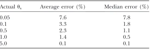
The methods we have developed in this article also allow us to estimate the distribution of selection pres-sures across sites. In one simple case discussed above, we have presented a procedure for estimating the number of lethal sites and the selective pressure operating on the remaining, nonlethal sites in a gene. This procedure involves estimatingganduson the basis of polymorphic sites alone and thereafter estimating the proportion of observed monomorphic sites that are lethal. To assess
the power and accuracy of this approach, Table 1 shows the error in the predicted number of monomorphic sites in each of our simulations, compared to the number of monomorphic sites actually observed. Across a large range of selective pressures and mutation rates, this approach typically estimates the number of (non-lethal) monomorphic sites within a few percent. As a result, for a gene of lengthL¼2000 sites, at one-half of which mutations are strongly deleterious (jsj?1=N), our procedure will accurately predict the number of lethal sites within a few percent, and it will accurately
Figure1.—Maximum-likelihood estimates of selection pressures obtained under the PRF method, the modified (per-site) PRF
method, and the three-dimensional diffusion method. Selection pressures were estimated from the folded polymorphism fre-quencies amongn¼14 sequences sampled from a simulated Wright–Fisher population. In each panel, the simulated selection pressureg is shown on thex-axis and the estimated selection pressure ˆgon they-axis. Dashed lines indicate 95% confidence intervals around the ML estimates obtained from thex2-distribution (seemethods). The line ˆg¼gis shown in red, and the line ˆ
predict the selection pressure on the remaining, non-strongly deleterious sites.
All of the simulation results that we have presented thus far have been for the casen¼14. This choice affects the relative accuracy of the methods. Asnincreases, the probability of seeing a high-frequency polymorphism within the sample depends more strongly on the probability that a site has a high-frequency polymor-phism in the population,f(x) for largex. This is precisely the part of frequency distribution that is artificially suppressed by the infinite-sites assumption of the PRF method. Thus, as the sample size increases the biases in the PRF method should become more severe. We have tested this expectation by samplingn¼100 simulated Wright–Fisher sequences. In the case ofus ¼ 0.1, for example, when fitting unfolded polymorphism fre-quency spectra measured relative to the (known) ancestral state at each site, the PRF method always rejects the true value ofgin favor of a weaker or even positive selection coefficient, throughout the rangeg2
[10, 0.5]. Inferential biases associated with large sample sizes and mutation rates will become increas-ingly important as the availability of sequence data improves—in metagenomic surveys of microbial pop-ulations, for example.
DISCUSSION
The Poisson random field model (Sawyer and
Hartl1992) and the associated likelihood procedure
for estimating parameters (Hartl et al. 1994) are
perfectly valid when the assumptions underlying the method are met—namely, infinite sites, free recombi-nation, and constant selective pressure across sites. Moreover, the assumption of infinite sites is perfectly reasonable for most eukaryotic populations. It will hold wheneverNmln½1=jsj>1; as we have seen, a rough rule of thumb is that this tends to be true whenus,0.05. We have shown, however, that when the mutation rate is relatively large the PRF method can lead to incorrect inferences. In practice, such concerns arise when studying populations of viruses, microbes, and those eukaryotes that experience large mutation rates (us. 0.05). We have developed two new methods that relax or remove the infinite-sites assumption. These new meth-ods also extend the types of inferences that can be drawn from polymorphism data to include inferences on the distribution of selective pressures across sites.
It may seem surprising that the infinite-sites approx-imation can lead to substantial errors in the mutation rates and selective strengths inferred by the PRF method. After all, sites at which multiple mutant lineages are sampled are presumably very rare (e.g., Hartl et al. 1994). Yet despite their rarity, these sites
have a large impact on maximum-likelihood estimation
of g. Because g enters the likelihood function in the
factore2gx, changingghas a much larger impact on the likelihood of sites with many mutant nucleotides than those with few. In other words, a single site with a high frequency of mutant nucleotides is very strong evidence for positive selection or lowjgj, whereas a site with a low frequency of mutant nucleotides is not very strong evidence for the opposite. Thus even a few sites at
Figure2.—Maximum-likelihood estimates of the mutation
rate,us¼2Nm, obtained under the PRF method (blue), the modified (per-site) PRF method (green), and the diffusion methods (red). Mutation rates were estimated from the folded polymorphism frequencies amongn¼ 14 sequences sampled from a simulated Wright–Fisher population. The simulated mutation rateusis shown on thex-axis and the es-timated mutation rate ˆus on the y-axis. The line ˆus¼us is shown in black. For each value of us, simulations and fits are shown for 17 different values ofg, ranging from g ¼ 10.0 tog¼ 0.1. The PRF method systematically underes-timates the mutation rate, especially when selection is weak. The diffusion method provides accurate and unbiased esti-mates of the mutation rate across the full range of parameters.
TABLE 1
Accuracy of the estimated number of monomorphic sites
Actualus Average error (%) Median error (%)
0.05 7.6 7.8
0.1 3.3 1.8
0.5 2.3 1.1
1.0 1.4 0.5
5.0 0.1 0.1
which multiple mutant lineages are sampled can cause large inaccuracies in the inferred g when they are incorrectly assumed by the original PRF method to be the result of a single high-frequency mutant lineage. These inaccuracies in g then force corresponding inaccuracies in the inferredus.
Previous simulation studies have not observed these problems with the PRF method (Bustamante et al.
2001). However, such simulations themselves implicitly assumed infinite sites, and hence they cannot be used to test this aspect of the PRF method (to be fair, these simulations were done with typical eukaryotic popula-tions in mind, where these problems are much less severe). In this article, by contrast, we have simulated a finite number of sites that evolve according to the Wright–Fisher model.
The role of linkage:While our focus has been on the
infinite-sites approximation, both the original PRF and all of our methods make another key assumption: that each site is independent of all the others (i.e., free recombination). This is essentially an assumption of linkage equilibrium between all polymorphic sites. This potentially crucial assumption is likely to be violated in many real populations, particularly when the method is applied to estimate selective pressure on short stretches of DNA (e.g., a single gene) that are linked over long timescales. This is problematic for both the original PRF and our methods, but it may be particularly relevant in populations in which finite-sites issues are important, because recombination is presumably less common in bacteria than in eukaryotes and because higher us implies a higher density of polymorphic sites, and hence tighter linkage. Ideally, we would address this assump-tion using theory that allows us to infer the strength of selection acting on a large number of sites with an arbitrary degree of linkage. However, this is a formida-ble challenge, and no such theory yet exists.
Despite this, models that assume free recombination are still useful for several reasons. First, when selection pressures are weak, sites segregate over long timescales, so recombination may be frequent enough even among intragenic sites (or in bacterial genomes) that segregat-ing sites are unlinked over these timescales. Since both PRF and diffusion-type methods are primarily useful at estimating selection pressures when they are of order 1/N, the selection pressures our methods can resolve get smaller asusincreases. Thus while populations with large us may tend to have lower recombination rates among polymorphic sites, the polymorphic sites we are sensitive to segregate over longer timescales, and re-combination has longer to act. Whether this means that linkage can be neglected in any particular population is an empirical question, but fortunately it is usually straightforward to estimate linkage disequilibria directly from the data. Thus in any particular case we can estimate whether or not the assumption of free re-combination is valid for the purposes of the original PRF
or our modified methods, before applying either approach. When there is no linkage disequilibrium in the data, we can use our methods with confidence. When on the other hand it appears from the data that free recombination is not a reasonable assumption, a model that assumes no linkage may still be useful as a null model and a limiting case, and it can be compared with more complicated possibilities.
Finally, it is important to note that linkage between segregating sites will not bias estimates of the selection pressureg, providedgis equal across sites (Akashiand
Schaeffer1997; Bustamanteet al.2001). Rather, the
primary effect of linkage is to increase the variance in such estimates above the predictions of our method (Bustamanteet al.2001). Thus while the predictions of
our models (or the original PRF) will tend to have smaller confidence intervals than they should, the estimated values ofgandusshould not be systematically biased. It is important to note, however, that when linkage is im-portant we must be cautious about testing hypotheses using these methods; underestimates of the confidence intervals could, for example, lead us to erroneously re-ject a neutral null. Further, when selection pressures vary significantly across sites, the mean parameter estimates themselves could be biased; this more complex situation remains an important topic for future exploration.
Comparison between the PRF and diffusion meth-ods:Our per-site version of the PRF model relaxes some aspects of the infinite-sites approximation, but it still as-sumes the mutant lineages do not interact. The diffusion approach removes the infinite-sites approximation alto-gether. Thus, the diffusion approach contains none of the biases associated with infinite-sites approximation associated with the traditional PRF and, to a lesser degree, the per-site PRF.
The diffusion method is also easily extendable to more complex evolutionary situations. For example, we can explore different selective costs for different nucleo-tides, or more than one preferred nucleotide. These possibilities lead to obvious modifications of the diffu-sion equations and their solutions and hence to the maximum-likelihood estimation. Mutational biases are more difficult to explore, as no simple steady-state solu-tion to the three-dimensional diffusion equasolu-tion exists for biased mutation rates, but computational results can still be obtained. It is also straightforward to investigate balancing selection or the effects of dominance: these lead to well-understood modifications to the diffusion equations and their steady-state solutions (Ewens2004).
The methods we have developed also allow us to relax the assumption of constantg across sites and instead infer aspects of the distribution of selection pressures (Piganeauand Eyre-Walker2003, Nielsenet al.2005,
and Boyko et al. 2008 have recently analyzed similar
extensions of the original PRF method). It is not yet clear how much data is required to provide adequate power for inferring this distribution to a given resolu-tion. However, we can hope to gain a great deal of insight with only a few additional parameters—say, the number of sites that are neutral, lethal, and negatively selected and the weighted average selection pressure on the latter class. As we have shown, we can estimate the number of lethal sites with no reduction in power relative to the original PRF method, so this proposal would involve only one additional parameter. Addi-tional classes of sites would involve more parameters. Eyre-Walker and Keightley (2007) have recently
stressed that the distribution of fitness effects of deleterious mutations is likely to be complex and multimodal. Using our approach, we can choose how to focus the power in the data to investigate the aspects of this complex distribution that are most interesting in a given situation. The appropriate choice of resolution will depend on the context and quality of the data.
However, the diffusion approach is not without draw-backs. The one-dimensional version does not make use of all of the data available in the observed polymor-phism spectrum and is likely to be of little use in practice because we typically do not know whether or not the ancestral nucleotide was preferred. The three-dimensional version uses all the data in the folded case, but cannot make use of outgroup data (the unfolded case). In practice, when we do not have an outgroup, the three-dimensional diffusion method provides the most accurate estimates of selection pressures across the full range of parameters. When an outgroup is available, the three-dimensional diffusion approach is still sometimes more accurate than the PRF, despite wasting informa-tion on the ancestral state, but only in parameter regimes typical of bacteria or viruses. In other cases the per-site PRF method is best.
The diffusion method also cannot naturally handle positive selection. The steady-state evolutionary dynam-ics at a site are always dominated by the preferred nucleotide (or nucleotides), with negative selection acting against polymorphisms for the disfavored nucleo-tides. At the level of an individual site, positive selection is a process that is intrinsically out of steady state: the spread of a favorable nucleotide before it becomes fixed. The PRF method handles positive selection by implicitly positing rather strange dynamics at individual sites. All mutant lineages are assumed to be positively selected—so if a mutant nucleotide fixes at a given site, mutations back to the ancestral nucleotide are again assumed to be positively selected (the analogous strange dynamics also apply to negative selection). While this
assumption makes little sense at a per-site level, it allows the PRF model to obtain a steady state across sites, provided positive selection is ongoing and not satu-rated. We could modify our diffusion methods to mimic the PRF treatment of positive selection by changing the boundary conditions in our diffusion equations. Specif-ically, we would assume that probability flowing intox¼
1 (i.e., fixation of a mutant nucleotide) is absorbed and moved tox¼0 (i.e., ‘‘reset’’ so that new mutations will again be favored). This diffusion equation can be solved exactly, and the solution used as a basis for inferring positive selection using the the per-site diffusion meth-ods we have developed.
Ideally, however, we want to infer positive selection in the context of a realistic and well-defined model of the dynamics at individual sites. Such an approach would necessarily involve full time-dependent solutions to the diffusion equations; Mustonen and Lassig (2007)
suggest a method along these lines. We do not pursue this approach here, but see Chenet al.(2007) for a step in
this direction. Regardless of the methodology, it will always be difficult to discriminate positive selection from negative selection on the basis of the polymorphism frequency spectrum alone, particularly when only folded data are available. Whether selection is positive or negative, mutant lineages drift nearly neutrally when their frequency is between 0 and 1/jgj. Positively selected lineages then fix relatively quickly once their frequency becomes substantially larger than 1/jgj, while negatively selected lineages rarely ever reach frequencies larger than 1/jgj. Thus from the point of view of the poly-morphism frequency spectrum, positive selection is similar to random drift on [0, 1/jgj], with the upper bound a roughly absorbing boundary condition. Nega-tive selection, on the other hand, is also similar to random drift on [0, 1/jgj], but with the upper bound a roughly reflecting boundary condition. Although this is relatively crude—selection does in fact have some impact on low-frequency lineages, and the boundary conditions are not exactly absorbing or reflecting—it indicates that the polymorphism frequency spectrum is roughly similar for negative and positive selection at the samejgj. Thus power to distinguish positive from negative selection based on the polymorphism frequency spectrum, espe-cially with folded data, will always be relatively limited, regardless of the method used.
Different steady states:The PRF framework and the
The differences in the nature of the two steady states are most readily apparent when considering their behavior for smallus. This is easiest to see by comparing the PRF steady state to the one-dimensional diffusion result (assuming as usual that one nucleotide is pre-ferred and the other three are unprepre-ferred). For small us, the population will typically be fixed for one of the four nucleotides. Occasionally mutations will occur, making the site temporarily polymorphic within the population. Usually these mutant lineages will drift at low frequency for a short while before going extinct, but occasionally they will fix and the population will be fixed for this new nucleotide. The PRF steady state describes the (transient) frequency spectrum of these occasional mutant lineages before they fix or go extinct. This spectrum is always measured relative to the ancestral nucleotide, which is the last mutation that fixed. On the other hand, the diffusion method describes the longer-term steady-state frequency distribution of the nucleotides. This includes some weight near x ¼ 0 (the preferred nucleotide is fixed, or nearly so), as well as some weight near x ¼ 1 (one of the unpreferred nucleotides is fixed, or nearly so). Because of the selective bias, the population will be fixed or nearly fixed for the preferred nucleotide a fraction 1=ð113e2gÞ of the time (Ewens2004), so 1=ð113e2gÞof the total
weight is in the part of the distribution nearx¼0. The remainder of the time, the population will be fixed or nearly fixed for one of the unpreferred nucleotides; this is the weight in the distribution nearx¼1.
The discussion above helps to elucidate the relation-ship between the steady states in the PRF modelvs.those in the diffusion model. A fraction 1=ð113e2gÞ
of the time the most recent fixation will have been for the preferred state. This is the ancestral state for the PRF method, and the frequency spectrum of the occasional unpreferred negatively selected mutants is given by the PRF steady state. The remainder of the time the most recent fixation will have been for one of the unpre-ferred states. Now this is the ancestral state for the PRF method, and the frequency spectrum of occasional mutants for the preferred nucleotide, which are under positive selection, is again given by the PRF steady state, but with the opposite sign ofg. Thus we expect that the diffusion method steady state is just the sum of these two PRF steady states, weighted by the frequency with which each type of nucleotide is the ancestral state, namely
fdiffðg;xÞ pðgÞfPRFðg;xÞ1½1pðgÞfPRFðg;1xÞ;
where p(g) denotes the chance that the most recent fixation was for the preferred state. This relationship between the two steady states is illustrated in Figure 3. It holds in the limit of small us. For larger us, the population is not always nearly fixed for one state. Mutant lineages occur more frequently and can segre-gate simultaneously (i.e., finite-sites effects). Since the diffusion approach accounts for this while the PRF does
not, the relationship between the steady states breaks down.
The difference between the diffusion and PRF steady states points to one additional bias in the PRF method that we have not yet discussed. Imagine a stretch of sequence that has been under constant purifying selection for an extremely long time. As we have just seen, we expect that at a fraction 3e2g=ð
113e2gÞ of the sites in this sequence, the most recent ancestor will be an unpreferred state. The PRF frequency spectrum at these sites will be characteristic of positive selection (mutations to the preferred nucleotides are beneficial). Although this will typically represent a minority of the sites, the PRF method weights sites under positive selection more strongly than those under negative selection when inferring a weighted average g. Thus, the PRF method will be biased toward inferring positive selection—despite the fact the sequence has experi-enced negative selection for an arbitrarily long time. This effect is present even for small us, and it is most severe when selection is weak but nonzero.
Whether this effect represents a bias in the PRF method is a matter of taste. In some sense, the PRF is
Figure 3.—Relationship between the PRF and diffusion