Monte Carlo simulation of a solvated ionic polymer with cluster morphology

Monte Carlo Simulation of a Solvated Ionic Polymer

With Cluster Morphology

Jessica L. Matthews

Department of Mathematics, North Carolina State University, Raleigh, NC, 27695, [email protected]

Emily K. Lada

Statistical and Applied Mathematical Sciences Institute (SAMSI), Research Triangle Park, NC, 27709-4006, [email protected]

Lisa M. Weiland

Center for Intelligent Material Systems and Structures, Department of Mechanical Engineering, Virginia Polytechnic Institute and State University, Blacksburg, VA, 24061, [email protected]

Ralph C. Smith

Center for Research in Scientific Computation, Department of Mathematics, North Carolina State University, Raleigh, NC, 27695, [email protected]

Donald J. Leo

Center for Intelligent Material Systems and Structures, Department of Mechanical Engineering, Virginia Polytechnic Institute and State University, Blacksburg, VA, 24061, [email protected]

Abstract

A multiscale modeling approach for the prediction of material stiffness of the ionic polymer Nafion is presented. Traditional rotational isomeric state theory is applied in combination with a Monte Carlo methodology to develop a simulation model of the conformation of Nafion polymer chains on a nanoscopic level from which a large number of end-to-end chain lengths are generated. The probability density function of end-to-end distances is then estimated and used as an input pa-rameter to enhance existing energetics-based macroscale models of ionic polymer behavior. Several methods for estimating the probability density function are compared, including estimation using Johnson distributions, B´ezier distributions, and cubic splines.

1. Introduction

the polymer matrix provides them with unique transduction capabilities for a variety of appli-cations. Specifically, mechanical deformations produce an internal redistribution of charges and solvent which produces a measurable electrical signal, thus giving the polymer sensing capabilities. Reciprocally, applying an electric field to the structure produces ionic migration toward the negative surface which, when combined with the redistribution of solvent, leads to bending in the structure, enabling the ionic polymer to act as an actuator. As an actuator, the material has greater actuation displacement and can be operated under much lower voltages than other electroactive materials (such as peizoelectric ceramics). These materials are superior to a number of existing transducers for several reasons, including their ability to operate under cryogenic conditions and their high gravimetric energy density. The growing number of potential applications for ionic polymers in-clude artificial robotic muscles and biomimetic sensors. A detailed review of the early history of these materials and their applications is provided by Shahinpoor et al. [17].

One factor inhibiting the widespread practical implementation of ionic polymers is the fact that many aspects of their behavior are not fully understood. In recent years, significant focus has been directed towards the development of suitable models which quantify their unique behavior. Several models have focused on characterizing the electromechanical response through the first principles of fluid transfer [1, 4, 6, 16]. Other models represent the mechanical deformation of ionic polymers as functions of current [1, 13] or ion transport [11]. Most recently, there has been progress on formulation of models which incorporate both the sensing and actuation properties of the material [14, 15].

In Weiland and Leo [23], an energetics approach is used to study the equilibrium state of the hydrophilic cluster regions of the ionic polymer Nafion. The primary goal of that work is to better understand how the equilibrium state may facilitate or inhibit ion transport as it relates to transduction. One significant drawback to that approach is the lack of appropriate nanoscale stiffness data. Moreover, multiscale stiffness predictions of ionomers in general, to date, have not been studied and represent an area critical to the tailoring of material response.

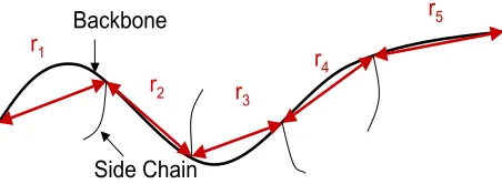
The overall goal of this investigation is to enhance the existing energetics-based models of ionic polymer behavior by estimating the material properties of the hydrophobic region of the material. Specifically, we focus on the development of a multiscale modeling approach for the prediction of material stiffness. This method involves the application of rotational isomeric state theory (RIS), traditionally used for studying deformation trends and material properties as described by Flory [8], in combination with a Monte Carlo methodology to develop a simulation model which characterizes the conformation of Nafion polymer chains. The material stiffness depends on multiple parameters including the effective length of the polymer chains comprising the material. This model will be used to simulate a large number of distancesr between cluster interaction points — that is, points where the ionic terminal groups for one pendant chain come within a certain distance of an embedded cluster. It is therefore assumed that communication between an ionic terminal group and a cluster acts as a crosslink. For the single Nafion chain in Figure 1, there are five cluster interaction points, resulting in the r values {ri :i= 1, . . . ,5}. The simulatedr-values can then be used to estimate a probability density function P(r) for cluster interaction distance (or equivalently, polymer chain length). Our modeling methodology is based on the approach of Mark and Curro [12] for short chain polymers displaying rubber elasticity and is similar to the application of the Mark–Curro method to study the effect of particle reinforcement in polymers, as described in [18, 19].

Relation of Density to Macroscopic Properties

r₁

r₅

r₄ r₃

r₂ Backbone

Side Chain

Figure 1: Distancesr between cluster interaction points for a single Nafion polymer chain.

through the expression

S(r) =klnP(r)

wherek is Boltzmann’s constant. Under the assumption of rubberlike elasticity, the “three chain” model as described by Treloar [20] may be applied to compute the change in entropy from an unperturbed configuration to a distorted configuration,

∆S= ν 3

S(roα) + 2S(roα−1/2)−3S(ro)

where ν is the number density of network chains, ro is the root mean square of the

simulation-generated r values and α = L/Li is the relative length of the sample. RIS theory assumes that under load, the rotation about a given bond is unrestricted and thus the Helmholtz free energy is strictly a function of entropy, allowing the nominal stressf∗ to be then given by

f∗ =−T

∂∆S ∂α

T

=−νkT ro 3

G(roα)−α−3/2G(roα−1/2)

, (1)

where G(r) = lnP(r) and G(r) = dG_dr(r). The corresponding modulus [f∗] is computed from the relation,

[f∗] = f

∗

α−α−2. (2)

is discussed in [22].

In addition to developing an appropriate simulation model for Nafion polymer chain conforma-tions as it relates to rotational isomeric state (RIS) theory, another significant goal of this paper is to investigate and compare several different methodologies for estimating the probability density function P(r). In Mark and Curro [12], a cubic spline approach is used to estimate P(r). Here, we present two alternative methods for estimating P(r) using the Johnson translation system of distributions [10] and B´ezier distributions [21]. While B´ezier curves offer a very flexible approach to density estimation with an open-ended parameterization that allows for the estimation of density functions with multiple modes, our results show that the estimates of P(r) obtained by fitting an appropriate Johnson distribution to the data are more intuitive than those obtained using B´ezier and cubic spline approaches for the following reasons. First, it is possible to write down an ex-plicit functional form for the Johnson density function that is simple to differentiate. This is a crucial property since the function will be used as an input to the mathematical model (1) and (2) to compute a Young’s modulus. The functional form of a B´ezier density is considerably more complicated than the Johnson and whereas a cubic spline density function has a simple form, its piecewise definition results in considerably more parameters to estimate than the globally-defined Johnson density function. Second when fitting a Johnson density function to the simulated data, one continuous curve is fit to the data so that infinite levels of differentiability are guaranteed. When fitting a cubic spline density, however, a piecewise-continuous curve is fit to the data — a property that may produce alternating second derivative signs, which ultimately can lead to neg-ative stiffness predictions, as shown in [22]. Furthermore, the piecewise nature of the cubic spline fit makes it difficult to accurately estimate the tails of the distribution.

synthesis stage.

The rest of this paper is organized as follows. The development of the simulation model for the atomic structure of the Nafion polymer backbone is described in Section 2, including details of the geometry of the Nafion backbone chain and the rotational isomeric scheme used to place backbone atoms in three-dimensional space. Section 3 includes descriptions of the cubic spline, Johnson, and B´ezier methods for density estimation as well as the results of applying these three methods to the simulation-generatedr values.

2. The Model

This paper focuses on the development of a Monte Carlo simulation model for the atomic structure of the Nafion polymer backbone chain with the ultimate goal of finding the probability distribution of side chain cluster interaction distances. Each iteration of the simulation produces a single Nafion molecule backbone within a cubic grid of dimension (5000 ˚A)3. The starting point of each chain is randomly specified and the backbone is dynamically constructed according to a commonly assumed geometry and under the restrictions that it cannot exceed the bounds of the initial grid or collide with the embedded clusters.

2.1. Geometry of the Nafion Backbone Chain

Bulk Nafion material is a complicated network of molecules. As a polymer, an individual Nafion molecule is composed of the monomer shown in Figure 2, which is repeatedmtimes. The−(CF2−

CF)(CF2−CF2)n- portion of the formula is collectively referred to as the backbone of the polymer.

The -(CF2 −CF2)n- portion, or Polytetrafluoroethylene (PTFE), is commonly known as Teflon.

3

CF |

− 3

−SO

2

−CF

2

−CF−O−CF

2

O−CF |

−

n

)

2

−CF

2

−CF)−(CF

2

− (CF

Figure 2: Structural formula of Nafion monomer.

2.1.1. Ranges for Nafion Monomer Variables

Since the structural formula for Nafion has not been published, the values ofnandm are sampled from a known range. The typical Nafion composition is 87/13, meaning that for every 87 (CF2CF2)

groups, there are 13 (CF2CF) groups comprising the polymer backbone. The actual values of n

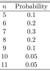
used in the simulation are drawn from the discrete probability distribution on the range [5,. . .,11] as summarized in Table 1. The probabilities in Table 1 were selected so that the distribution forn would be nearly symmetric with a mean of approximately 87/13≈7.

Preliminary research also suggests that there exists substantial variation in chain length for Nafion polymers. The total molecular weight bounding cases of 150,000 and 250,000 g/mol were em-ployed to arrive at a reasonable range formto account for this variation of molecular chain length. Using the standard atomic masses for carbon (12.0107), fluorine (18.9984), oxygen (15.9994), and sulfur (32.0650), the mass of each (CF2CF) portion of the polymer backbone with the attached

side chain is 443.1161 g/mol. When taken in conjunction with the 87/13 composition of Nafion, approximately 40% of the total molecular weight is produced by the (CF2CF) portions of the

poly-mer backbone along with the attached side chains. Upon examination of the bounding cases, we

Table 1: Discrete probability distribution fornvalues. n Probability

5 0.1

6 0.2

7 0.3

8 0.2

9 0.1

10 0.05

see that 0.40×150,000/443.1161 ≈ 135 and 0.40×250,000/443.1161 ≈ 225. Hence, the m values used in the simulation were uniformly drawn from integers in the range [135,. . .,225].

While this is the target range for the repeated monomer units, the simulated chains are termi-nated at much shorter lengths due to chain collision with a cluster. Actual simulated chain lengths m ranged between 1 and 45 with a typical value of 4. Whereas early termination clearly leads to non-physical predictions of total chain lengths, it is not believed that early termination presents a significant problem in the estimation ofP(r) because it is the distance between cluster interactions which dictate the elastic properties of the material.

2.1.2. Bond Length and Angles of Bond Orientation

The initial model focuses on characterizing the backbone of the polymer. From standard chemistry principles, the length of a carbon-carbon bond from the centers of both atoms is known to be l= 1.53 ˚A [8]. This fixed bond length was used throughout the simulation as the distance between backbone chain atoms.

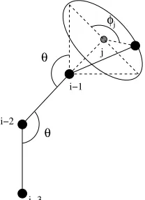
Since the simulation is performed in three-dimensional space, there are two angles required for the placement of any backbone atom. These are the valence angleθ between successive bonds and the angle of rotationφfor each bond. For our purposes, the valence angle (like the bond length) is considered to be a fixed quantity for all pairs of successive bonds. Due to the large proportion of PTFE in the backbone, well-established PTFE values are applied throughout. In particular, the valence angleθ is fixed at 116o. The parameter of experimental interest is the angle of rotationφ.

θ θ

φj

i−3 i−2

i

i−1 j

Figure 3: Spatial geometry of a Nafion molecule.

For simplicity, when placing an atom i, the simulation temporarily performs the necessary rotations and translations to place the backbone atom i−1 at the origin, atom i−2 along the negative x-axis of the Cartesian coordinate grid, and atom i−3 in the negative x–negative y quadrant of the x-y plane. Once in this configuration, atom imay be placed locally by randomly selecting an angleφj and measuring clockwise from the point on the base of the cone in the positive x–positive yplane, as shown in Figure 4. Specifically, the local Cartesian coordinates of atomiare defined by

  

xi yi zi

 

 =

  

·cos(θ) ·cos(−φj)·sin(θ) ·sin(−φj)·sin(θ)

  

where is the carbon-carbon bond length of 1.53 ˚A andθ is the supplementary angle toθ having the value of 180−θ= 64o. After placing atomilocally, the inverse of the rotations and translations applied to the positions of atomsi−1,i−2, and i−3 to achieve the local configuration in Figure 4 are performed on atomiso that it is in the correct position with respect to the remainder of the backbone chain before temporarily rotating atoms i−1, i−2, andi−3.

2.2. Rotational Isomeric Scheme

Although the conformational characteristics of PTFE or Teflon (the predominant structure in the Nafion backbone) are well represented by a three-state model with rotation angles of one trans

θ θ φj x i j i−2 i−3 z y i−1

Figure 4: Local geometry of a Nafion molecule after temporarily rotating atoms i−1,i−2, and i−3 for the purpose of placing atomi.

angles of two trans (φ=±15o) and two gauche (φ=±120o) conformations.

2.2.1. Statistical Weight Matrices

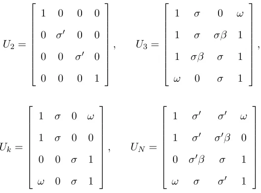
From [7], it is known that the given rotational state of any bond in a polymer depends on the rotational state of its neighboring bonds . The first-neighbor dependence was incorporated into this simulation by invoking a statistical weight parameteru(α, η, j) =uα,η,j whereαis the state of the preceding bond,ηis the state of the current bond, andj is the location of the bond within the molecular chain. Therefore, adapting from the values for the statistical weight parameters arrived at by Bates and Stockmayer in [3], we employ the matrixUj = [uα,η,j] for bond j, where

U2 =

         

1 0 0 0

0 σ 0 0 0 0 σ 0

0 0 0 1

         

, U3=

         

1 σ 0 ω

1 σ σβ 1

1 σβ σ 1

ω 0 σ 1

          ,

Uk=

         

1 σ 0 ω

1 σ 0 0

0 0 σ 1

ω 0 σ 1

         

, UN =

         

1 σ σ ω

1 σ σβ 0 0 σβ σ 1 ω σ σ 1

          .

the range for each of the values provided in [3] and the associated energy values. Note that all of the above matrices are indexed in the ordert+ (15o),g+ (120o),g− (-120o), and t− (-15o) on both the rows and columns. Furthermore, since the first bond is placed randomly, we have included U2

to place the second bond of the backbone, U3 to place the third bond of the backbone, and UN to place the last bond of the entire backbone chain. Hence Uk is used to place bonds 4≤k≤N −1, where N = 2(m+m_p=1np)−1 is the total number of bonds in the backbone chain andnp is the pth randomly generated value of nfrom the range [5, . . . ,11], as described in Section 2.1.1.

2.2.2. Conditional Probability Matrices

The stochastic element of the Monte Carlo simulation of the atomic structure of Nafion focuses on determining the angle of rotation φ for each bond. However, the statistical weight matrices Uj, 2 ≤ j ≤ N derived in the previous section are non-normalized. Therefore, we must use the similarity transformation

Qj =ε−j,11D− 1

j,1UjDj,1,

where εj,1 is the largest eigenvalue of Uj and Dj,1 is the diagonal matrix of the elements of the

eigenvector associated with εj,1, to normalize each of theUj to obtain the conditional probability matrices [8],

Q2=

         

1 0 0 0 0 1 0 0 0 0 1 0 0 0 0 1

         

, Q3 =

         

0.6552 0.2137 0 0.1310 0.4017 0.1310 0.0655 0.4017 0.4017 0.0655 0.1310 0.4017 0.1310 0 0.2137 0.6552

          ,

Qk =

         

0.7295 0.1246 0 0.1459

0.8541 0.1459 0 0

0 0 0.14589 0.8541

0.1459 0 0.1246 0.7295

         

, QN =

         

0.2781 0.4829 0.2144 0.0245 0.3203 0.5562 0.1235 0

0 0.6263 0.0556 0.3181 0.1261 0.1095 0.4863 0.2781

          .

bond in the entire molecular chain and each Qj is indexed in the order t+ (15o), g+ (120o), g− (-120o), andt− (-15o) on both the rows and columns. Note that the rows of the above matrices do not sum exactly to unity since each value has been truncated in the interest of space. It is these conditional probability matrices which are employed to choose the angle of rotationφfor all bonds in the simulation based on the rotational state of the preceding bond, where in the actual code the untruncated values are used so that each row sums exactly to unity. For example, suppose we are attempting to place the last bond of a backbone chain where the preceding bond is in thet+

state. This indicates that the first row of QN contains the appropriate conditional probabilities to select the particularφvalue for the current bond. A random number generator is invoked to select a random number between 0 and 1. Assume a value of 0.4 is returned. Since 0.278≤0.4≤(0.278 + 0.482), we have randomly selected the valueφN = 120o.

2.3. Initial Grid Orientation

As noted previously, the space within which the molecular chains are constructed is of dimension (5000 ˚A)3. The standard Cartesian coordinate system is oriented so that the range of values along each of the x, y, and z axes is [-2500, 2500]. These dimensions were chosen so that the longest possible molecule, according to the maximum m and mean n values of the Nafion formula, when fully extended, could be contained within the grid.

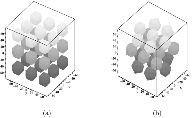
It is of particular interest in this investigation to examine the effects of embedded inclusions upon the cluster communication distances. In this simulation, the embedded inclusions are hydrophilic clusters in which the side chains tend to terminate and which are assumed to already exist as though the grid was populated with other Nafion molecules. This simplified model considers the clusters to be spherical in shape and uniformly distributed throughout the grid [9]. Since it is difficult to arrive at a truly uniform distribution of spheres on a rectangular grid where the centers of the spheres are equidistant from each other, two possible grid orientations were considered: rectangular (analogous to cubic crystalline structure) and staggered (analogous to hexagonal close packed (HCP) crystalline structure), as shown in Figure 5.

–60 –40 –20 0 20 40 60

x –60

–40 –20 0

20 40

60 y –60

–40 –20 0 20 40 60

–60 –40 –20 0 20 40 60

x –60

–40 –20

0 20

40 60 y –60

–40 –20 0 20 40 60

(a) (b)

Figure 5: (a) Rectangular grid orientation, and (b) staggered grid orientation.

the choice of volume fraction of the entire grid occupied by the clusters. The radius of the spherical clusters and the volume fraction of the total grid they occupy were varied to examine several specific cases. The first of these is the case where the 1100 Equivalent Weight Nafion material is fully hydrated with water and sodium is used as the cation. Under these conditions, the clusters each have a radius of 21 ˚A and the total volume fraction of the clusters is 30%, based on results from Bar-Cohen [2]. From these characteristics, the center-to-center distance between clusters for both the rectangular and staggered orientations is 2.4×radius = 50.4 ˚A. In the second case, we assumed that the 1100 Equivalent Weight Nafion material is fully hydrated with water and lithium is used as the cation. These conditions result in a radius of 23 ˚A and the total volume fraction of the clusters to be 38%, based on results from Bar-Cohen [2]. These values imply a center-to-center distance between clusters for both the orientations to be 2.2×radius = 50.6 ˚A.

2.4. Variations for Backbone Atoms with Side Chains

2.4.1. Atom Placement

hydrophobic molecule, there exists a tendency for the terminal groups and the water absorbed by the material to cluster together. We choose to incorporate this phenomenon into the simulation by overriding the conditional probability matrices used to chooseφ(as described in Section 2.2.2) and instead use theφ-value that would place the backbone atom with the attached side chain closest to an embedded cluster. This is accomplished by forming all possible orientations produced by each of the ±15o and ±120o rotation angles and computing the distances to the nearest clusters. Once the minimum distance is found, the associated angle of rotation φ is used to actually place the backbone atom with the attached side chain using the same method described in Section 2.1.2.

2.4.2. Achieving Side Chain Cluster Communication

It was noted previously that the goal in this characterization technique is to quantify the distance between cluster interaction points along the Nafion molecular backbone. At every backbone atom with an attached side chain, there is an opportunity for a cluster interaction point, meaning that the attached side chain terminal group comes into communication with an embedded cluster. This cluster communication is assumed to occur when the backbone atom with an attached side chain is within a distance of 8 ˚A of an embedded cluster. The cluster communication distance of 8 ˚A was determined by examining the composition of the attached side chains. Although they may take on a number of conformations and hence lengths, the maximum length is approximated as 8 ˚A. Therefore, the backbone atoms which achieve side chain-cluster communication are tracked such that successful cluster communication is assumed to act as a crosslink. Our end result is comprised of computing the distances between these subsequent backbone atoms, as well as the endpoints of the molecular chain.

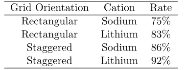
Table 2: Successful cluster communication rates. Grid Orientation Cation Rate

Rectangular Sodium 75% Rectangular Lithium 83% Staggered Sodium 86% Staggered Lithium 92%

clusters, this would also suggest higher success rates due to tighter cluster packing. Furthermore, although we have employed the cluster communication distance of 8 ˚A, only approximately 10% of the successful cluster interactions occur when the backbone atom with the attached side chain is between 6.5 ˚A and 8 ˚A from the nearest cluster. Hence the bulk of the simulated cluster interac-tions occur at minimal distances, which is critical due to the fact that 8 ˚A is an assumed maximum value.

3. Simulation Results

The simulation model was run for each of the following four cases: sodium as the cation with a rectangular grid orientation, sodium as the cation with a staggered grid orientation, lithium as the cation with a rectangular grid orientation, and lithium as the cation with a staggered grid orientation. For each of the four cases, a data set of approximately 10,000rvalues was generated by simulating possible conformations of the Nafion backbone, using the method described in Section 2. We then estimated the probability density functionP(r) using two methods: Johnson distributions and B´ezier functions. In the Sections 3.2 and 3.3, we will detail the steps followed to estimateP(r) using each of these two methods. First, however, we will describe the traditionally applied cubic spline method for density estimation.

3.1. Fitting Data with Cubic Splines

a knot value is specified for each bin so that on each interval (delimited by the knots), a cubic polynomial is fit to the data. If we define the indicator functionLi(r) for the subinterval (ki, ki+1],

whereki is the ith knot, as

Li(r) =

    

1, forki < r≤ki+1,

0, otherwise,

(3)

then the result is a piecewise-polynomial estimate of P(r) of the form

P(r) = 1 K

n∗

i=1

Li(r)

Ai(r−ki)3+Bi(r−ki)2+Ci(r−ki) +Di

, (4)

wheren∗ is the number of knots,A, B, C, andDare the estimated coefficients, andK is a normal-izing constant so that the function P(r) given in (4) integrates to unity.

The advantage to using cubic splines for density estimation is that the resulting function has a simple form and can easily be applied in mathematical models to describe various material properties. One challenge with this approach is that cubic polynomials are often not sufficiently flexible to accurately model the tail behavior of the density. Additionally, the shape of the estimated density is highly dependent on the number and location of the knots. For instance, if the number of knots is large, then the corresponding estimate of P(r) may be excessively noisy. Finally, the details of the fitting methodology are typically not well-defined and often a trial-and-error approach is necessary to determine the number and location of the knots.

−200 0 20 40 60 80 100 0.01

0.02 0.03 0.04 0.05 0.06 0.07 0.08

r

P(r)

knots

Estimated Cubic Spline PDF Simulated PDF

Figure 6: Estimated cubic spline PDF for the sodium/rectangular case.

chain lengths.

3.2. Fitting Data with Johnson Distributions

The Johnson translation system of distributions [10] is comprised of four flexible families of dis-tributions including lognormal, unbounded, bounded, and normal which cover a wide variety of distribution shapes. It is this flexibility which makes the Johnson system an attractive option to estimate P(r) from the simulated data for polymer chain length.

If X is the continuous random variable whose distribution is to be estimated, the cumulative distribution function (CDF) ofXisF(x) = Pr{X≤x}and the probability density function (PDF) of X is P(x) = F(x). Johnson developed a method for estimating the unknown densityP(x) by transforming the random variable X into a standard normal random variable,

Z=γ+δf

X−ξ λ

,

f(y) =                   

ln(y), for theSL (lognormal) family, ln(y+y2_{+ 1), for theS}

U (unbounded) family, ln(₁₋y_y), for theSB (bounded) family, y, for theSN (normal) family.

(5)

The corresponding PDF for X is

p(x) = δ λ√2πf

x−ξ

λ exp −1 2

γ+δ·f

x−ξ λ

2

(6)

for all x∈Hwheref(·) is the first derivative of the functionf(·) in (5) and the (closed) support of the distribution is

H=                   

[ξ,+∞) for theSL (lognormal) family, (−∞,+∞) for theSU (unbounded) family, [ξ, ξ+λ] for theSB (bounded) family, (−∞,+∞) for theSN (normal) family.

The software package FITTR1 [24] incorporates several methods for fitting Johnson distribu-tions, including moment matching, percentile matching, ordinary least squares (OLS), diagonally weighted least squares (DWLS), L1-norm and L∞-norm estimation for each of the four families.

Descriptive statistics (including mean, standard deviation, skewness, and kurtosis) of the sample data, goodness-of-fit information, as well as tables of the empirical and fitted CDF and PDF for plotting are available outputs of the FITTR1 package.

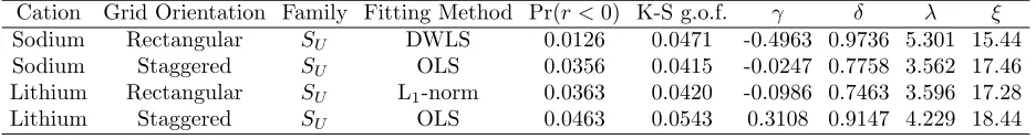
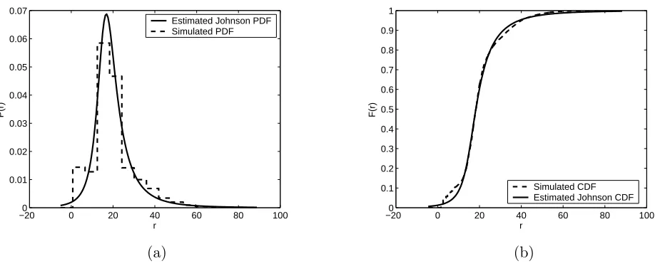
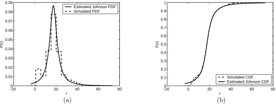
each of the four simulated cases, estimates of P(r) were generated using various combinations of Johnson families (primarily the bounded and unbounded) and fitting methods. Based on the Kolmogorov-Smirnov statistic and plots of the estimated Johnson PDF and CDF versus the data, one fit was selected as the “best” fit for each of the four cases (see Figures 7–10). Table 3 provides the corresponding parameter estimates and the Kolmogorov-Smirnov goodness-of-fit statistic (K-S g.o.f.) for the Johnson distributions shown in Figures 7–10.

Although our goal is to determine an estimate of P(r), the PDF for the cluster interaction distances r, we select the best fit primarily by comparing plots of the empirical CDF versus the fitted Johnson CDF since the empirical PDF, which is often represented as a histogram, is highly subjective and the shape can vary greatly depending on the choice of histogram cell width. For example, if the width of the histogram bars are taken to be very small, the resulting estimate of the PDF may be excessively noisy or bumpy (that is, it may contain extraneous bumps or modes that are a function of the randomness of the simulation and may not actually be features of the true underlying PDF). Conversely, if the width of the histogram bars are taken to be very large, the resulting estimate of the PDF may be over smoothed and important features of the true PDF may be lost.

When studying the plots of the empirical versus the fitted CDF, we consider two main regions: the middle section (10< r <30) and the tail sections (r <10 and r >30). Of greater importance is the closeness of fit in the middle section since this region characterizes the bulk of the cluster communication distances. As seen in Figures 7–10, we were able to successfully fit the middle portion of the data using a Johnson unbounded distribution for each of the four cases. Accuracy while fitting the tail sections is also desired, however it is difficult in this case to get a close fit in the lower tail since the fitted Johnson density is continuous and the data in the lower tail

Table 3: Parameter estimates for the fitted Johnson unbounded distribution for each of the four simulated cases.

Cation Grid Orientation Family Fitting Method Pr(r <0) K-S g.o.f. γ δ λ ξ

Sodium Rectangular SU DWLS 0.0126 0.0471 -0.4963 0.9736 5.301 15.44

Sodium Staggered SU OLS 0.0356 0.0415 -0.0247 0.7758 3.562 17.46

Lithium Rectangular SU L1-norm 0.0363 0.0420 -0.0986 0.7463 3.596 17.28

is discrete. For those r values computed for backbone subchains with a very small number of bonds (less than 5), there is only a small number of combinations of atom placement since there are only four angles of rotation to choose from. For example, if the formation of the backbone chain terminates after the placement of the second carbon atom, then a value of r = 1.53 will be recorded, corresponding to the length of one carbon-carbon bond. Similarly, if the backbone chain terminates after the placement of the third carbon atom, then a value ofr = 2.595, corresponding to the distance between the ends of 2 carbon-carbon bonds, will be recorded. If the backbone chain terminates after the placement of the fourth atom, then there are only four possible resulting r values corresponding to each possible value of the rotation angle φ. As the number of bonds in a backbone subchain increases, the distribution of r values begins to look more continuous since there are increasingly more combinations of atom placement and hence chain lengths.

−200 0 20 40 60 80 100

0.01 0.02 0.03 0.04 0.05 0.06 0.07

r

P(r)

Estimated Johnson PDF Simulated PDF

−200 0 20 40 60 80 100

0.1 0.2 0.3 0.4 0.5 0.6 0.7 0.8 0.9 1

r

F(r)

Simulated CDF Estimated Johnson CDF

(a) (b)

−200 0 20 40 60 80 0.01 0.02 0.03 0.04 0.05 0.06 0.07 0.08 0.09 r P(r)

Estimated Johnson PDF Simulated PDF

−200 0 20 40 60 80

0.1 0.2 0.3 0.4 0.5 0.6 0.7 0.8 0.9 1 r F(r) Simulated CDF Estimated Johnson CDF

(a) (b)

Figure 8: Estimated PDF (a), and CDF (b) for the sodium/staggered case using a Johnson un-bounded density function.

−200 0 20 40 60 80

0.01 0.02 0.03 0.04 0.05 0.06 0.07 0.08 0.09 r P(r)

Estimated Johnson PDF Simulated PDF

−200 0 20 40 60 80

0.1 0.2 0.3 0.4 0.5 0.6 0.7 0.8 0.9 1 r F(r) Simulated CDF Estimated Johnson CDF

(a) (b)

Figure 9: Estimated PDF (a), and CDF (b) for the lithium/rectangular case using a Johnson unbounded density function.

−100 0 10 20 30 40 50 60 70

0.01 0.02 0.03 0.04 0.05 0.06 0.07 0.08 0.09 r P(r)

Estimated Johnson PDF Simulated PDF

−100 0 10 20 30 40 50 60 70

0.1 0.2 0.3 0.4 0.5 0.6 0.7 0.8 0.9 1 r F(r) Simulated CDF Estimated Johnson CDF

(a) (b)

Another critical drawback to the Johnson unbounded fits in Figures 7–10 is that there is a significant nonzero probability that the fitted Johnson density could generate anr value less than zero, as seen in Table 3. To correct this, we attempted to fit a Johnson bounded distribution to the data for each of the four cases. The fitted CDF and PDF for the Johnson bounded fits are shown in Figures 11–14 and Table 4 gives the K-S g.o.f. statistic and the parameter values for each of the four cases. The lower bound for each case was set to zero. Clearly, while the Johnson bounded fits have a zero probability of generating a negativer value, the fits are not as accurate as the Johnson unbounded fits. Since the lower bound is fixed, the Johnson bounded distribution only has three parameters to estimate, rendering it even less flexible than the Johnson unbounded distribution.

Despite these drawbacks, however, the Johnson distribution still provides an accurate estimate of the density of polymer chain length, requiring the estimation of only four parameters. Furthermore, the functional form of the Johnson PDF in (6) can easily be used as an input to the macroscopic-level model given by (2) to predict material stiffness. As indicated in [22], the estimated Johnson density functions for chain length result in stable and repeatable stiffness predictions.

−200 0 20 40 60 80 100

0.01 0.02 0.03 0.04 0.05 0.06

r

P(r)

Estimated Johnson PDF Simulated PDF

−200 0 20 40 60 80 100

0.1 0.2 0.3 0.4 0.5 0.6 0.7 0.8 0.9 1

r

F(r)

Simulated CDF Estimated Johnson CDF

(a) (b)

−200 0 20 40 60 80 0.01 0.02 0.03 0.04 0.05 0.06 0.07 0.08 r P(r)

Estimated Johnson PDF Simulated PDF

−200 0 20 40 60 80

0.1 0.2 0.3 0.4 0.5 0.6 0.7 0.8 0.9 1 r F(r) Simulated CDF Estimated Johnson CDF

(a) (b)

Figure 12: Estimated PDF (a), and CDF (b) for the sodium/staggered case using a Johnson bounded density function.

−200 0 20 40 60 80

0.01 0.02 0.03 0.04 0.05 0.06 0.07 0.08 r P(r)

Estimated Johnson PDF Simulated PDF

−200 0 20 40 60 80

0.1 0.2 0.3 0.4 0.5 0.6 0.7 0.8 0.9 1 r F(r) Simulated CDF Estimated Johnson CDf

(a) (b)

Figure 13: Estimated PDF (a), and CDF (b) for the lithium/rectangular case using a Johnson bounded density function.

−100 0 10 20 30 40 50 60 70 0.01 0.02 0.03 0.04 0.05 0.06 0.07 0.08 r P(r)

Estimated Johnson PDF Simulated PDF

−100 0 10 20 30 40 50 60 70 0.1 0.2 0.3 0.4 0.5 0.6 0.7 0.8 0.9 1 r F(r) Simulated PDF Estimated Johnson PDF

(a) (b)

Table 4: Parameter estimates for the fitted Johnson bounded (SB) distribution for each of the four simulated cases.

Cation Grid Orientation Family Fitting Method K-S g.o.f. γ δ λ ξ

Sodium Rectangular SB OLS 0.0797 2.760 2.076 87.96 0

Sodium Staggered SB OLS 0.1041 2.721 2.385 72.19 0

Lithium Rectangular SB L1-norm 0.1050 3.059 2.495 78.23 0

Lithium Staggered SB OLS 0.1205 1.910 2.138 57.29 0

3.3. Fitting Data with B´ezier Distributions

Although the Johnson translation system of distributions is remarkably flexible, it is limited by the fact that only four parameters are available to control the shape of the fitted distribution. Alternatively, the B´ezier distribution family offers an open-ended parameterization technique which enables it to accurately represent nearly any possible distributional shape [21]. This characteristic enables the fitted B´ezier curve to characterize the behavior in the tails of the empirical distribution more precisely.

B´ezier curves are a special class of spline curves used to approximate a smooth univariate func-tion on a bounded interval by forcing the curves to pass through the vicinity of selected control points {pk ≡(xk, zk)T :k = 0,1, . . . , n}. Visually, the control points can be interpreted as ‘mag-nets’, exerting a ‘magnetic attraction’ which forces the B´ezier curve towards them. In particular, the first and last control points are interpolated exactly, meaning that the B´ezier curve will pass through these points. It should be noted that changing the location of any control point affects the shape of the entire curve. Every control point pk provides two parameters, specifically the xk and zk coordinates. Hence, if a B´ezier curve of degree n is used, we have n+ 1 control points and 2n parameters.

A B´ezier curve of degreen with control points{p0,p1, . . . ,pn}is parametrically written as

P(t) = [Px(t;n, x), Pz(t;n, z)]T

= n

k=0

Bn,k(t)pk for t ∈[0,1],

Bn,k(t)≡

    

n!

k!(n−k)!tk(1−t)n−k, for t ∈ [0,1] andk= 0,1, . . . , n,

0, otherwise.

If X is a (continuous) B´ezier random variable with bounded support [x_∗, x∗], the cumulative distribution function (CDF)FX[x(t)] can be approximated to arbitrary accuracy by a B´ezier curve with sufficiently high degree n. Hence, the CDF is given parametrically by

P(t) = [Px(t;n, x), Pz(t;n, z)]T

= {x(t), FX[x(t)]} for all t∈ [0,1]

where the control points {p0,p1, . . . ,pn} are placed so as to adhere to the basic requirements of a CDF—that is, FX(·) is monotonically nondecreasing, FX(x∗) = 0 and FX(x∗) = 1. Given this representation of the CDF, the corresponding probability density function (PDF) fX[x(t)] = F_X [x(t)] is given parametrically by

P∗(t) = [P_x∗(t;n, x), P_z∗(t;n, x, z)]T

= {x(t), fX[x(t)]} for all t ∈[0,1].

(7)

Here

P_z∗(t;n, x, z) = Pz(t;n−1,z) Px(t;n−1,x) ,

x≡(x0, . . . ,xn−1)T,

z≡(z0, . . . ,zn−1)T,

and xk ≡ xk+1 − xk and zk ≡ zk+1 −zk(k = 0,1, . . . , n−1) are taken to represent the

corresponding differences of the x- and z- coordinates of the control points in the parametric representation of the CDF.

To fit a B´ezier distribution to the simulated data for each of the four cases, we use the graphical software package PRIME. Among the fitting methods available in PRIME are moment match-ing, percentile matchmatch-ing, maximum likelihood, least squares, L1- and L∞-norm estimation. After

ad-equate fit, or the user can interactively choose both the number and location of the control points. Descriptive statistics, goodness-of-fit information (including the Kolmogorov-Smirnov statistic), as well as plots of the empirical and fitted CDF and PDF are available outputs of the PRIME software package. For additional details about the PRIME software, see [21].

For each of the four cases of simulated data detailed in Section 2.3, two interactive B´ezier distribution fits were performed. The first fit for each case uses 6 control points (requiring the estimation of 10 parameters) while the second fit uses 12 control points (requiring 22 estimated parameters). Figures 15 and 16 show the B´ezier fits for the sodium/rectangular case using 6 control points and 12 control points, respectively. The fits in these figures are indicative of the fits obtained for the other three simulated cases. The K-S goodness-of-fit statistic is 0.01996 for the fit with 6 control points and 0.01535 for the fit with 12 control points. Compared to the K-S goodness-of-fit values for the corresponding Johnson fits in Tables 3 and 4, the B´ezier fits appear to provide a more accurate fit to the simulated data since the maximum discrepancy between the empirical and fitted CDFs is much smaller for the B´ezier fits.

From Figure 16 it is evident that if enough control points are used, it is possible to fit the simulated (empirical) data very closely using a B´ezier function. At the same time, however, it may not be desirable to track the empirical data exactly. For example, the empirical data in Figure 16 suggests there may be a second mode in the lower tail of the distribution. If enough control points are used, it is possible to capture the bimodal behavior of the data using a B´ezier density function. Physically, however, there is not any evidence to suggest that the underlying true density of cluster communication distances is bimodal. As a result, it is not clear that the B´ezier fits provide a better estimate ofP(r) than the Johnson fits in Figures 7–14.

0 20 40 60 80 100 0 0.01 0.02 0.03 0.04 0.05 0.06 0.07 0.08 0.09 r P(r)

Estimated Bezier PDF Simulated PDF

0 20 40 60 80 100

0 0.1 0.2 0.3 0.4 0.5 0.6 0.7 0.8 0.9 1 r F(r)

Estimated Bezier CDF Simulated CDF

(a) (b)

Figure 15: Estimated PDF (a), and CDF (b) for the sodium/rectangular case using a B´ezier function with 6 control points.

0 20 40 60 80 100

0 0.01 0.02 0.03 0.04 0.05 0.06 0.07 0.08 0.09 r P(r)

Estimated Bezier PDF Simulated PDF

0 20 40 60 80 100

0 0.1 0.2 0.3 0.4 0.5 0.6 0.7 0.8 0.9 1 r F(r)

Estimated Bezier CDF Simulated CDF

(a) (b)

Figure 16: Estimated PDF (a), and CDF (b) for the sodium/rectangular case using a B´ezier function with 12 control points.

4. Concluding Remarks

theory. In order to achieve this goal an expression for P(r) which is both accurate and easily manipulated mathematically is required.

Thus, in addition to proposing an appropriate simulation for multiscale study of Nafion stiffness, in this paper we have also proposed two methods for estimating the probability density function P(r) as alternatives to the cubic spline method used in [12]. Both the proposed Johnson and B´ezier density estimation methods provide a more flexible approach to density estimation than the cubic spline method. Furthermore, while using B´ezier curves to estimate P(r) offers a highly flexible technique for estimating a wide variety of distribution shapes, the Johnson family of distributions have a simple four-parameter functional form. Additionally, the parameters of the Johnson dis-tribution have a specific physical meaning and current research efforts are focusing on identifying relationships between the Johnson parameters and predicted stiffness.

Acknowledgements

The authors would like to thank James Wilson (North Carolina State University) for many en-lightening discussions regarding the estimation of density functions using Johnson and B´ezier dis-tributions. Collaboration was facilitated while the authors were visitors at the Statistical and Applied Mathematical Sciences Institute (SAMSI), Research Triangle Park, NC, and the research of EKL was supported in part by the Science Foundation through the SAMSI grant DMS-0112069. LMW and DJL were supported by National Science Foundation Grant CMS 0093889 whereas RCS was supported in part by the Air Force Office of Scientific Research through the grant AFOSR FA9550-04-1-0203. The authors gratefully acknowledge this support.

References

[1] Asaka K, Oguro K, Nishimura Y, Mizuhata M and Takenaka H 1995 Bending of polyelectrolyte membrane–platinum composites by electric stimuli, part I. Response characteristics to various waveformsPolymer Journal 27436–40

[3] Bates T W and Stockmayer W H 1968 Conformational energies of Perfluoroalkanes, part II. Dipole Moments ofH(CF2)nH Macromolecules 1 12–17

[4] Brock D, Woojin L, Segalman D and Witkowski W 1994 A dynamic model of linear actuator based on polymer hydrogelProc. Int. Conf. on Intelligent Materials 210–22

[5] DeBrota D J, Dittus R S, Roberts S D, Swain J J, Venkatraman S and Wilson J R 1989 Modeling input processes with Johnson distributions Proc. Winter Sim. Conf. (Piscataway, NJ: Institute of Electrical and Electronics Engineers) 308–18

[6] de Gennes P G, Okumura K, Shahinpoor M and Kim K J 2000 Mechanoelectric effects in ionic gels Europhysics Letters 50(4) 513–18

[7] Flory P J 1953Principles of Polymer Chemistry, (Ithaca, NY: Cornell University Press)

[8] Flory P J 1989Statistical Mechanics of Chain Molecules (NY: Hanser Publishers)

[9] Hsu W Y and Gierke T D 1982 Elastic theory for ionic clustering in perfluorinated ionomers

Macromolecules 15101–05

[10] Johnson N L 1949 Systems of frequency curves generated by methods of translationBiometrika

36(1/2) 149–76

[11] Li J Y and Nemat-Nasser S 2000 Micromechanical analysis of ionic clustering in Nafion per-fluorinated membraneMech. Mater. 32303–14

[12] Mark J E and Curro J G 1983 A non-Gaussian theory of rubberlike elasticity based on rota-tional isomeric state simulations of network chain configurations, part I. Polyethylene and poly-dimethylsiloxane short-chain unimodal networksJournal of Chemical Physics 79(11) 5705–09

[13] Mojarrad M and Shahinpoor M 1997 Ion-exchange metal composite artificial muscle actuator load characterization and modeling Proc. SPIE Smart Materials and Structures Conf.;SPIE Publication 3040294–301

[14] Nemat-Nasser S and Li J Y 2000 Electromechanical response of ionic polymer-metal composites

Journal of Applied Physics 87(7) 3321–31

[16] Segalman D, Witkowski W, Adolf D and Shahinpoor M 1991 Electrically-controlled polymeric gels as active materials in adaptive structuresProc. of ADPA/AIAA/ASME/SPIE Conf. On Active Materials and Adaptive Structures 335–45

[17] Shahinpoor M, Bar-Cohen Y, Simpson J O and Smith J 1998 Ionic polymer-metal composities (IPMCs) as biomimetic sensors, actuators and artificial muscles–a reviewSmart Materials and Structures 7(6) R15–R30

[18] Sharaf M A, Kloczkowski A and Mark J E 2001 Monte Carlo simulations on reinforcement of an elastomer by oriented prolate particles.Comp. Theo. Poly. Sci.11251–262

[19] Sharaf M A and Abouhussein R H 2003 Computer simulations on the chain deformations of poly(ethylene) by randomly-oriented prolate filler particles arranged on a cubic latticePoly. Preprints 44(1) 1258–9

[20] Treloar L R G 1975The Physics of Rubber Elasticity, 3rd ed. (Oxford: Clarendon Press)

[21] Wagner M A F and Wilson J R 1996 Using univariate B´ezier distributions to model simulation input processesIIE Transactions 28699–711

[22] Weiland L M, Lada E K, Smith R C and Leo D J 2004 Application of rotational isomeric state theory to ionic polymer stiffness predictionsJournal of Materials Research (in review)

[23] Weiland L M and Leo D J 2005 Computational analysis of ionic polymer cluster energetics

Journal of Applied Physics (to appear)