Selection for Environmental Variation: A Statistical Analysis and Power Calculations to Detect Response

DOI: 10.1534/genetics.108.091678

Selection for Environmental Variation: A Statistical Analysis and Power

Calculations to Detect Response

Noelia Iba´n

˜ez-Escriche,*

,†,‡

_{Daniel Sorensen,}

‡,1

_{Rasmus Waagepetersen}

§

_{and Agustı´n Blasco*}

*Departamento de Ciencia Animal, Universidad Polite´cnica de Valencia, 46071 Valencia, Spain,†Gene`tica i Millora Animal, Centre IRTA

Lleida, 2598 Lleida, Spain,‡Department of Genetics and Biotechnology, Faculty of Agricultural Sciences, University of Aarhus, DK-8830 Tjele, Denmark and§Department of Mathematical Sciences, University of Aalborg, DK-9220 Aalborg, Denmark

Manuscript received May 18, 2008 Accepted for publication September 19, 2008

ABSTRACT

Data from uterine capacity in rabbits (litter size) were analyzed to determine whether the environmental variance was partly genetically determined. The fit of a classical homogeneous variance mixed linear (HOM) model and that of a genetically structured heterogeneous variance mixed linear (HET) model were compared. Various methods to assess the quality of fit favor the HET model. The posterior mean (95% posterior interval) of the additive genetic variance affecting the environmental variance was 0:16ð0:10;0:25Þ and the corresponding number for the coefficient of correlation between genes affecting mean and variance was0:74ð0:90;0:52Þ. It is argued that stronger support for the HET model than that derived from statistical analysis of data would be provided by a successful selection experiment designed to modify the environmental variance. A simple selection criterion is suggested (average squared deviation from the mean of repeated records within individuals) and its predicted response and variance under the HET model are derived. This is used to determine the appropriate size and length of a selection experiment designed to change the environmental variance. Results from the analytical expressions are compared with those obtained using simulation. There is good agreement provided selection intensity is not intense.

T

HE classical model of quantitative genetics assumes that genotypes affect the mean of a trait but that the environmental variance (variance of phenotype, given genotype) is the same for all genotypes. An extension postulates that both mean and variability differ between genotypes (San Cristobal-Gaudy et al. 1998). The

extended model has interesting implications in animal and plant improvement (e.g., Hill and Zhang2004;

Mulder et al. 2007) since it offers the possibility to

decrease variation by selection leading to more homo-geneous products. In evolutionary biology, a central problem is to understand the forces that maintain phenotypic variation. With the exception of recent work (Zhangand Hill2005), most of the models assume that

environmental variance is constant and explain the level of phenotypic variation by invoking a balance between the gain of genetic variance by mutation and its loss by different forms of selection and drift.

Early evidence for a genetic component affecting environmental variation stems from comparison of levels of variation between inbred lines and the F1cross between them, with inbreds showing in general larger variance (reviewed in Falconer and Mackay 1996).

More recent evidence has come from fitting the model to

data on litter size in pigs (Sorensenand Waagepetersen

2003), adult weight in snails (Roset al. 2004), body weight

in poultry (Roweet al. 2006), slaughter weight in pigs

(Iba´ n˜ ezet al. 2007), and litter size and weight at birth

in mice (Gutierrezet al. 2006). Stronger, more direct

support, not derived from fitting the genetically struc-tured heterogeneous variance model, but from analyses of experiments with isogenic chromosome substitution lines of Drosophila, was provided by Mackayand Lyman

(2005). Here, homozygote inbred lines that differed in chromosome 2 or 3 were created, and variation between individuals in abdominal and sternopleural bristle num-ber was computed. Difference in within-line variance, between lines, was confirmed. Since individuals within a line are effectively replicates of the same genotype, difference in within-line variance, between lines, provides evidence for the presence of genes located in chromo-somes 2 and 3 affecting environmental variance.

With the exception of experimental organisms such as Drosophila and some plant or fish species where replicated individuals of the same genotype (clones) can be produced and variation between individuals composing the clone measured directly, support for the presence of genes controlling environmental varia-tion can be found, fitting the model to data and studying the quality of the fit using modern computational tools. Stronger support would entail showing that the envi-ronmental variance responds to selection pressure in an appropriately designed experiment. The latter requires 1_{Corresponding author: Department of Genetics and Biotechnology,}

Faculty of Agricultural Sciences, University of Aarhus, PB 50, DK-8830 Tjele, Denmark. E-mail: [email protected]

to define an observable that properly reflects environ-mental variation and to determine the expected change of this observable due to selection and its variance in conceptual replications. This knowledge is needed to design an adequate experiment.

There are two objectives in this work. The first is to provide new results in favor of the existence of genetic variation at the level of environmental variance. Litter size in repeated parities in rabbits is taken as an example. Two models are fitted; one assumes homogeneity of environmental variance and the other postulates a genetically structured variance heterogeneity. The models are compared contrasting the quality of their fit, using posterior predictive model checking (Gelman et al. 1996), using cross-validation (Gelfand1996), and

using the deviance information criterion, an index that encapsulates the fit of a model and its complexity (Spiegelhalteret al. 2002). The second objective is to

derive expressions to predict response to selection for environmental variance, and the variance of the re-sponse, with the purpose of studying a number of issues concerning the design and size of experiments to detect this response.

STATISTICAL ANALYSIS OF LITTER SIZE DATA

Data:The data originate from a selection experiment for uterine capacity in rabbits (litter size in unilateral ovariectomized does; technique described in Santacreu et al. 1990) spanning 10 generations. Uterine capacity is referred to as litter size hereinafter. Details of the selection experiment need not concern us here and can be found in Argenteet al. (1997). From the point of

view of the validity of inferences using selected data, it is important to emphasize that all the data used to make selection decisions have been included in the analyses reported in this work. Therefore the condi-tions for ignorability of selection under a Bayesian (or likelihood) analysis are met (Rubin1976; Littleand

Rubin1987).

Animals were derived from a synthetic population of the experimental farm at the Universidad Polite´cnica de Valencia that had undergone several generations of random mating before the start of the experiment. Reproduction was organized in discrete generations and mating of close relatives was avoided to reduce inbreed-ing. Females were first mated at 18 weeks of age and thereafter 10 days after parturition, producing in total up to four parities.

The total number of records was 2996. The number of animals in the pedigree was 1161; 85 of these composed the base population.

Models fitted and implementation: Data were ana-lyzed with two models. The first model assumes homo-geneity of environmental variance; the second assumes that the environmental variance is partly genetically determined. Both assume that the conditional

distribu-tion of the sampling model for the data is Gaussian, despite the fact that the trait in question is in the form of counts. Sorensenand Waagepetersen(2003)

investi-gated the consequences of this assumption by discretiz-ing data that had been simulated under the normal model. The normal model was fitted to the discretized data and the posterior distribution of the parameters agreed well with the values used to simulate the data.

Model 1is the classical repeatability additive genetic model. It assumes that the sampling model of the data vectory¼(yi)n

i¼1, given location parametersb,a, andp and given the residual variances2

e, is the normal process

yjb;s2

e NðXb1Za1Wp;Is2eÞ; ð1Þ

wherebcontains year–season effects with 30 levels (each level included 3 months, from spring 1991 until summer 1998) and parity order effects with 4 levels (first, second, third, and fourth or higher parities). Vectors a andp

contain additive genetic values (1161 levels) and per-manent effects (929 levels), respectively, ands2

e is the residual variance. The known incidence matrices areX,

Z, andWandIis the identity matrix.

Vectors p and a were assumed to be a priori in-dependently and normally distributed; that is,

pjs2

p Nð0;Is2pÞ; ð2Þ

ajs2

a Nð0;As2aÞ; ð3Þ

where A is the known additive genetic relationship

matrix. The vector b was assigned an unbounded

uniform prior distribution and the variance compo-nents s2

p, s 2

a, and s 2

e, scaled inverted chi-square distributions.

Under this model, the phenotypic variance is the variance of the conditional distribution ofyigivenband the variance components,

Var½yijb;s2a;s2p;s2e ¼s2a1s2p1s2e ð4Þ

and the heritability is

h2 ¼ s

2 a

s2

a1s2p1s2e

: ð5Þ

This model assumes homogeneity of environmental variation. It was fitted using a Gibbs sampling algorithm, as described, for example, in Sorensenand Gianola

(2002).

Model 2postulates that the environmental variance is heterogeneous and partly under genetic control. It assumes that conditionally on vectors of location and dispersion parameters, the vector of phenotypes is Gaussian,

yjb;a;p;b*;a*;p* Nðm;diagððs2_iÞn

where diag((s2

i)ni¼1) is the diagonal matrix with di-agonal entriess2

i,

ðlns2_iÞn

i¼1¼Xb*1Za*1Wp*;

and

m¼ ðm_iÞn

i¼1 ¼Xb1Za1Wp:

The vectorsbandb* contain effects associated with year– season and parity order and X, Z, and W are known incidence matrices. Vectorspandp* contain permanent environmental effects and are assumed to be indepen-dently distributed with normal structures

pjs2_p Nð0;s2_pIÞ ð7Þ

p*js2

p* Nð0;s2p*IÞ: ð8Þ

Vectors (aT_,

a*T_{) contain normally distributed additive}

genetic effects;i.e.,

a a*

jG N 0

0 ;G5A

; ð9Þ

where

G ¼ s2a rsasa*

rsasa* s2a*

:

Above, r is the coefficient of genetic correlation between a and a*, and ðs2

a;s2a*Þ are additive genetic variances associated with the distribution ofða; a*Þ. As discussed in Sorensen and Waagepetersen (2003),

this model generates a stochastic relationship between mean and variance when jrj , 1, a deterministic re-lationship when jrj ¼ 1, and absence of relationship whenr¼0.

Under this model, the phenotypic variance is the variance of the conditional distribution ofyigivenb,b* and the variance components

Var½yijb;b*;s2a;s2p;s2e;s2a*;s2p*

¼s2

a1s2p1exp ðXb*Þi1

s2_a*

2 1

s2_p* 2

!

; ð10Þ

where (Xb*)iis theith entry ofXb*. The heritability is

defined as

h_i2¼ s

2 a

s2_a1s2_p1expððXb*Þ_i1s2_a*=21s2_p*=2Þ: ð11Þ

There is one heritability for each combination of environmental effects (Xb*)i affecting the

environ-mental variance. More details can be found in Sorensen and Waagepetersen (2003) and in Ros et al. (2004).

The third central moment under model 2 is

E ðyi ðXbÞiÞ3jb*;s2a;s2a*;s2p*;r

h i

¼3rs_as_a*exp

ðXb*Þ_i1s

2 a*

2 1

s2_p* 2

ð12Þ

(Ros _{et al}. 2004). The conditional distribution of _yi

has therefore negative, zero, or positive coefficient of skewness

E ðyi ðXbÞ_iÞ3jb*;s2a;s2a*;s2p*;r

h i

Var yijb;b*;s2a;s2p;s2e;s2a*;s2p*

h i3=2; ð13Þ

depending on the value ofr. There is one coefficient of skewness for each combination of environmental effects (Xb*)iaffecting the environmental variance.

Details of the a priori distributions and the Markov chain Monte Carlo (MCMC) implementation to fit model 2 are described in Sorensenand Waagepetersen

(2003). Briefly, a priori,b andb* were assigned normal distributions with zero mean vector and diagonal co-variance matrix with very large diagonal elements. The variance parameterss2

a,s 2 a*,s

2 p, ands

2

p* were assigned scaled inverted chi-square distributions and r was as-signed a uniform prior bounded between1 and 1. The implementation was based on the MCMC algorithm proposed by Sorensen and Waagepetersen (2003).

Vector b was sampled using a Gibbs update, vectors (aT_,

a*T_{) and (}

pT_,

p*T_{) were reparameterized with the}

intention of reducing their posterior correlation and subsequently sampled using the Metropolis–Hasting algorithm with a Langevin–Hastings proposal, and the log-variance components and the correlation co-efficient were sampled using Metropolis–Hastings with random-walk proposals.

MODEL CHECKING AND MODEL COMPARISON

The three approaches described below to question the validity of the models address different questions. The deviance information criterion (DIC) provides a comparison of the global quality of two or more models, accounting for model complexity. Cross-validation based on conditional predictive ordinates (CPOs) provides a more detailed inspection, disclosing which specific data points are better fitted by the models. In addition, the set of CPOs contains the same information about model performance as the Bayes factor (Besag

to capture specific putative features of the data. In so doing, it suggests ways in which the model may be expanded to account for scientifically relevant aspects of the data.

An informal visualization of mean–variance relation-ship:The 929 females with records were sorted accord-ing to their mean litter size (across parities) and divided into 11 groups of85 individuals. Mean litter size and average variance between records within individuals were computed for each group. To visually explore a possible association between mean and variance, the average group variances were plotted against the group averages sorted in increasing order.

Posterior predictive model checking:A technique for checking the fit of a model to observed datayis to draw simulated values yrep from the posterior predictive distributions of replicated data and compareyrepwith the observed data (Rubin 1984; Gelman et al. 1995).

Any systematic differences between the observed and the simulated data indicate potential failings of the model. More specifically, the idea is to define a so-called discrepancy measureTðy;uÞthat depends on the data and perhaps also onu, an unknown parameter of the model under scrutiny, the null model, say. This measure

Tis specifically designed to test a particular feature of the dataythat may be of scientific relevance. Replicated data are then simulated from the posterior predictive distribution, given the null model, from which

Tðyrep;uÞ is constructed and compared with Tðy;uÞ. Differences between theT’s may be due to sampling or due to the inability of the null model to account for the feature of the observed data disclosed by the discrep-ancy measureT.

In this study we are concerned with studying hetero-geneity of environmental variation due to year–season effects, due to parity, and finally due to additive genetic effects. This was accomplished using the discrepancy measures proposed by Sorensenand Waagepetersen

(2003). Thus, effects of year–season and parity on variance heterogeneity were investigated using the discrepancy measure

Tj;lðy;u1Þ ¼

1

mj;l

X

Lij¼l

ðyimiÞ2

s2_i 1

; ð14Þ

wherejis an index for the two covariates, year–season and parity,l¼1,. . .,njis an index for thenjlevels of the

jth covariate, andLij¼lif theith record belongs to the

lth level of thejth covariate. The vectoru1contains the parameters of model 1,mjlis the number of the records with levellfor the jth covariate,mi is theith element

in Xb 1 Wp 1 Za, and ðyim_iÞ2_=s2

i is the squared

standardized residual associated with record i. Since the expected value of (14) is zero (see Sorensen and

Waagepetersen 2003), large or small values of Tj_,l

indicate possible variance heterogeneity due to thejth covariate.

A possible association between environmental varia-tion and additive genetic values affecting mean litter size was studied using the discrepancy measure

Tjðy;u1Þ ¼

1

mIj X

i:ai2Ij

ðyimiÞ2

s2 i

; j ¼1;. . .7; ð15Þ

wheremIjis the number of observations withai2Ijand

Ij ¼ tj;tj11

are subintervals of the real line with‘¼

t1 ,. . ., t7 ¼‘whose length was chosen to accom-modate a similar number of observations in each (425). Thus,Tjmeasures the average environmental variation in each group, where the groups are obtained by choosing the observations according to the size of their additive genetic values. The seven subintervals are ordered from the smallest group of additive genetic values (subinterval 1) to the largest (subinterval 7). A trend inTjplotted against the seven subintervals would be indicative of an association between environmental variation and additive genetic values affecting mean litter size.

Since random effects and other parameters involved in the construction ofTare unknown, one uses the idea of posterior predictive model checking (Rubin 1984;

Gelman et al. 1996) and considers the posterior

pre-dictive distribution ofTj(y,u₁)Tj(yrep,u1).

Cross-validation:Gelfandet al. (1992) propose using

a cross-validation (leave-one-out) approach based on posterior predictive distributions as a means of check-ing the fit of the model and in model choice. Let yi

denote datumi, and letyibe equal to the data vectory

with datumyideleted. That is,

yi¼ ðy1;. . .;yi1;yi11;. . .;ynÞ:

The posterior predictive density ofyiconditional onyi

and on modelMris

pðyijyi;MrÞ

¼

ð

pðyijyi;ur;MrÞpðurjyi;MrÞdur: ð16Þ

Very often,pðyijyi;ur;MrÞ ¼pðyijur;MrÞ. Withndata

points, there arenposterior predictive densities (Equa-tion 16). Note that the observedyi is not included to determine (16). The densitypðyijyi;MrÞevaluated at

the observed datumyiis also known as the conditional predictive ordinateðCPOiÞ,

CPOi¼pðyijyi;MrÞ: ð17Þ

If the model holds,yimay be viewed as a random draw from ½Yijyi;Mr whose density is given by (17). The

CPOi’s can be plottedvs. ias an outlier diagnostic, since

data having low CPOi’s are poorly fitted by the model.

Such a plot, for different models, discloses which model does better and which points are poorly fitted under the different models. A Monte Carlo estimate of (17) is

CˆPOi¼

1

m

Xm

j¼1

1

pðyijuðrjÞ;MrÞ

1

ð18Þ

(Gelfandet al. 1996). In the above expressions,uðjÞ r is

the jth MCMC draw from ½urjyi;Mr and m is the

number of draws (length of chain). An attractive feature of (18) is that it does not require implementing a new Bayesian analysis for eachyi.

Deviance information criterion:Spiegelhalteret al.

(2002) have introduced the DIC as a means of compar-ing models. The DIC uses the posterior expectation of the log-likelihood as a measure of model fit. For a particular modelM, the DIC is defined as

DIC¼2DDðu_MÞ; ð19Þ

where

D¼ 2

ð

lnpðyju_MÞ

pðu_Mjy;MÞdu_M

¼EuMjy½DðuMÞ ð20Þ

is the posterior expectation of the so-called deviance

DðuMÞ ¼ lnpðyjuMÞ. The term DðuMÞ in the

right-hand side of (19) is the deviance evaluated at the posterior mean of the parameter vectoruM. The term

D measures the quality of fit of a model, whereasD

Dðu_MÞis related to the ‘‘effective’’ number of parame-ters (Spiegelhalteret al. 2002). Expression (19) is the

result of combining both terms. Models having a smaller DIC should be favored as this indicates a better fit and a lower degree of model complexity.

DIC is very easily calculated using the MCMC output. The first term in the right-hand side of (19) is estimated using twice the average of the simulated values of

lnpðyjuMÞ, and the second term is estimated as the

deviance evaluated at the average of the MCMC simu-lated values ofuM.

RESULTS OF THE STATISTICAL ANALYSIS

Results corresponding to models 1 and 2 are based on 1,000,000 samples drawn using the appropriate MCMC

algorithm. To give an idea of the accuracy of Monte Carlo computations we report below confidence inter-vals for various Monte Carlo estimates of posterior means derived from model 2.

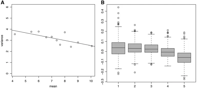
Variance components and heritability: Table 1 shows Monte Carlo estimates of posterior means and of 95% posterior intervals for variance components derived from models 1 and 2. The additive variances2

ais a little higher and the permanent environmental variances2

pa little lower in the case of model 2. The posterior mean of the correlation coefficient is 0.74; the Monte Carlo estimate of the 95% posterior interval indicates that the support of the posterior distribution is shifted a long way from zero (see also Figure 5B).

Monte Carlo estimates of features of posterior distri-butions are subject to Monte Carlo sampling error. Estimates of sampling error yield the following 95% con-fidence intervals for estimates of posterior means under model 2:ð0:78;0:86Þs2

a,ð0:42; 0:46Þs 2

p,ð0:76;0:73Þ r,ð0:15;0:16Þs2

a*,ð0:12;0:12Þs 2

p*. These intervals show that the length of the chain (sample size) used to esti-mate the posterior means results in adequate accuracy. Under model 1, the posterior mean (and 95% posterior interval) of the environmental variance is 4.37ð4:11;4:63Þ. Under model 2, the smallest posterior mean of the environmental variance and 95% posterior interval, corresponding to year–season 30 and parity 1, is 2.83ð2:61;3:10Þ. The corresponding largest number, for year–season 15 and parity 3 is 6.99ð6:61;7:26Þ.

The posterior mean and the 95% posterior interval of heritability of litter size under model 1 are 0.09 and

ð0:05;0:15Þ, respectively. Under model 2, there is one heritability for each combination of environmental effects (Xb*)i(see Equation 11) affecting the residual

variance. The average heritability over all combinations of environmental effects is 0.13 with a minimum of 0.09 (year–season effect 15 and parity order 3) and a maximum of 0.19 (year–season effect 30 and parity order 1). The 95% posterior intervals for these quanti-ties areð0:06;0:13Þandð0:13;0:25Þ, respectively.

Marginal posterior distributions of s2 a, s

2 a*, s

2 p, and s2

p* are shown in Figure 1. The superimposed lines represent densities of the prior nSx2_{-scaled inverted} TABLE 1

Monte Carlo estimates of posterior means (first row for each model) and of 95% posterior intervals (second row for each model) of variance components derived from models 1 and 2

Model s2

a s

2

p r s

2

a* s

2 p*

1 0.59 0.51 — — —

0.32; 0.86 0.28; 0.8 — — —

2 0.82 0.44 0.74 0.16 0.12

0.48; 1.28 0.20; 0.72 0.90;0.52 0.10; 0.25 0.07; 0.18

s2 aðs

2

a*Þ, additive variance at the level of the mean (variance);s 2 pðs

2

chi-square distributions of the variances. The posterior distributions in the four leftmost graphs (Figure 1A) were obtained using priors with parametersn¼4 and

S ¼ 0.45. The four rightmost posterior distributions (Figure 1B) were obtained using priors with parameters n¼4 andS¼0.05. The two sets of prior distributions have modal values of 0.300 and 0.033. The graphs indicate that posterior inferences of s2

a, s 2 a*, s

2 p, and s2

p* derived from model 2 are affected little by the choice of prior.

Deviance information criterion: The Monte Carlo estimates of the DICs for models 1 and 2 are 7810 and 7719, respectively. Based on 10 replicates, the respective Monte Carlo standard deviations are 0.23 and 0.27, respectively. Smaller values of the DIC indicate a ‘‘better’’ model. Thus, the DIC favors model 2.

Cross-validation: Figure 2A shows the difference in CPOs between model 2 and model 1, where the CPOs are sorted from the smallest to the largest for the 2996 records. For approximately two-thirds of the data there

is very little difference in the CPOs for both models. However, for the remaining one-third of the data, model 2 shows a better fit. Figure 2B shows which points are best fitted by model 2. The data are ordered from the smallest to the largest value of litter size. There is wide overlap for both models, with the excep-tion of observaexcep-tions in the center of the distribuexcep-tion, where model 2 results in a better fit than model 1.

Graphical assessment of genetic variance heteroge-neity: Results from the exploratory analysis based on posterior predictive model checking are shown in Figures 3 and 4. To test for environmental variance heterogeneity due to year–season, data were simulated under the homogeneous variance model (model 1) and the discrepancy measure Tys,l(yrep, u1) was computed [see expression (14)]. The difference between the discrepancy measure evaluated using the observed data,

Tys,l(y, u1), and the one evaluated using the simulated data is shown in Figure 3A. A similar exercise was carried out to study environmental variance heterogeneity due

Figure1.—(A) Monte Carlo estimates of s2

a ands 2

p (top) ands 2 a* and s

2

p* (bottom). The lines represent the prior scaled invertednSx2_{-densities with parametersn¼4 andS¼0.45. (B) The same as in A but with prior parametersn¼4 andS¼0.05.}

Figure 2.—(A)

to parity order (Figure 3B). Due to posterior uncertainty of the discrepancy statistic, Figure 3A) does not convey a clear message. It is difficult to conclude from this exploratory analysis whether there is evidence in the data for heterogeneity of variance due to year–season. On the other hand, the picture emerging from Figure 3B is that parity orders 1 and 2 seem to be associated with smaller environmental variance than parity orders 3 and 4.

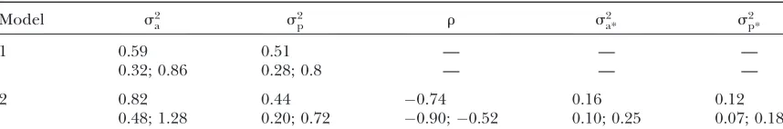
A graphical display of the relationship between the variance between records within individuals and litter size, sorted in increasing order, using a simple plot that does not involve fitting parametric models (see An informal visualization of mean–variance relationship), is shown in Figure 4A. A linear regression was fitted and the estimate is0.23 (standard error 0.07), indicating that as litter size increases, the variation among records within an individual decreases.

Figure 4B is in the same spirit as Figure 4A but is based on residuals computed from model 1. This enables filtering out variation due to fixed effects and genetic values affecting the mean and hence a more

precise look at the possible genetic variance heteroge-neity. The boxplots in Figure 4B obtained from MCMC samples of the posterior predictive distributions ofTj

Tjrep_{exhibit a decreasing trend that in accordance with}

the Figure 4A is indicative of a negative association between environmental variation and additive genetic values affecting litter size, as postulated by model 2. This is in good agreement with the posterior distribu-tion of the correladistribu-tion coefficient in Figure 5B (see also Table 1), whose support is in the negative real line, clearly shifted away from the valuer¼0. More details on this approach to posterior predictive model check-ing are provided in Sorensen and Waagepetersen

(2003).

Figure 5A shows a histogram of estimated residuals from model 1. The distribution is skewed to the left, in agreement with the coefficient of skewness (12) derived under model 2.

In conclusion, this model-fit study using different approaches favors the genetically structured environ-mental variance model 2 relative to the homogeneous environmental variance model 1.

Figure3.—(A) Boxplots

for posterior predictive re-alizations of discrepancy measure designed to test environmental variance het-erogeneity due to year– season,Tys,l(y,u2)Tys,l(yrep,

u2), l¼ 1,. . ., 30. (B) Box-plots for posterior predictive realizations of discrepancy measure designed to test environmental variance het-erogeneity due to parity or-der,Tpo,l(y,u2)Tpo,l(yrep,

u₂),l¼1,. . ., 4.

Figure _4.—(A)

SELECTION FOR ENVIRONMENTAL VARIANCE

The results of a study of two interrelated issues are presented in this section. First, an expression is derived to predict response to selection for environmental variance using the average sums of squares between records within individuals as a criterion of selection. This requires an experiment where repeated measure-ments are taken for each individual. We believe that a selection experiment should be designed in such a way that inferences could be drawn using simple approaches and particularly without explicitly invoking a model for variance heterogeneity to interpret the results. The criterion for selection proposed above can in principle fulfill this goal.

The second problem that is studied involves the size of the experiment required to detect a given change in environmental variance. The response to selection and the variance of the criterion of selection across concep-tual replications of the experiment are derived under a relatively simple version of the heterogeneous variance model. This is used to calculate the power to detect response. The results are compared with those obtained using simulated data.

Response to selection for environmental variance:

An expression for the expected response to selection is derived, where the selection criterion or index is the variance between repeated records within individuals. We consider a scenario that mimics selection for re-duced variation in litter size in repeated parities (such as in pigs, mice, or rabbits) and records are therefore available on females only. A hierarchical mating struc-ture is assumed, with Nm males, Nf females (Nf/Nm females mated to each male). Litter size is considered a trait of the female not influenced by the father of the litter. The index is computed for each female, and the males and females of the next generation are chosen among the unscored offspring from the best-scoring females of theNfscored.

As in Sorensen and Waagepetersen (2003),

con-sider the simplified version

yjb;a;b*;a* Nðb1a;expðb*1a*ÞÞ

and

ða;a*Þ js2_a;s_a*2 ;r N ð0;0Þ; s 2

a rsasa*

rsasa* s2a*

" #!

ð21Þ

of the genetically structured heterogeneous variance model, where b and b* are common to all records. Assume a simple scenario where there are availablen

records ðyjÞ, j¼1, 2,. . .,n per individual, on a large number of unrelated individuals. The goal is to reduce the variance among repeated records within individuals, and the criterion of selection is the empirical index I

defined as the variance of records within individuals

I ¼ 1

n1

X

j

ðyjyÞ2; n.1; ð22Þ

where y¼P_jyj=n. When selection with average in-tensity between sexes i operates on the index (22), calculations detailed in the appendix show that the

expected genetic mean (at the level of the environmen-tal variance) among the selected individuals is

Ra* ¼ i s

2 a*

ffiffiffiffiffiffiffiffiffiffiffiffiffiffiffiffiffiffiffiffiffiffiffiffiffiffiffiffiffiffiffiffiffiffiffiffiffiffiffiffiffiffiffiffiffiffiffiffiffiffiffiffiffiffiffiffiffiffiffiffiffiffi

expðs2_a*Þððn11Þ=ðn1ÞÞ 1

q : ð23Þ

There are two sources of inaccuracy contributing to (23). The first is associated with the linear approximation to truncation selection based on (A3) (seeappendix),

which is expected to deteriorate with increasing selec-tion intensity. Second, since the marginal distribuselec-tion of the index (22) is not normal, use of the standard values of i based on normality introduces another source of error. The accuracy of (23) is studied below using simulated data.

Figure5.—(A)

Distribu-tion of residuals computed from model 1. (B) Marginal posterior distribution of r

How does the expected change in the unobservable

a* based on (23) translate into an expected change in the observable (22)? Consider the second-order Taylor expansion

EðIjb*;a*Þ ¼expðb*1a*Þ

expðb*Þ 11a*1a

*2

2

: ð24Þ

In the absence of selection, taking expectation with respect to the distribution ofa*,

EðIjb*Þ expðb*Þ 11s

2 a*

2

; ð25Þ

since Eða*Þ ¼0 and Eða*2_{Þ ¼s}2

a*. With selection, ig-noring changes in s2

a*, Eða* 2_{Þ ¼s}2

a* and the expecta-tion of (24) can be approximated as

EsðIjb*Þ expðb*Þ 11Esða*Þ1s

2 a*

2

: ð26Þ

The expected change in the index (22) due to the ex-pected change ina* or expected response to selection in the index,RI, is, approximately,

RI¼EsðIjb*Þ EðIjb*Þ expðb*ÞEsða*Þ; ð27Þ

whereEsða*Þis given by (23). The estimated response to selection in the index is simply the difference between the two average indexes and is labeledRˆI. Formula (27) can be interpreted as an expected difference either involving a selected line and the base population or involving a selected and a control line. It holds provided that there are common nongenetic effects b and b* affecting all records. The expected difference in the average index (22) (over individuals, within lines) given by (27) includes the unknown nongenetic parameterb* acting on the environmental variance, but does not include the nongenetic parameterbacting on the mean. In the classical homogeneous variance model, the expected difference in phenotypic means between a selected and a control line is free from nongenetic generation effects provided that these affect the se-lected and control lines in the same manner. The dependence of the expected response to selection on the unknown parameterb* need not concern us here. As shown below, expressions for determining the size of the experiment are free fromb*.

A more realistic model would allow for possibly different nongenetic effects affecting records at the level of the mean and environmental variance. For example, for a particular individual the vector of n

recordsy¼ ðy1;y2;. . .;ynÞTcould be assumed to be the result of the sampling process

yjb;b*;a;a* NðXb11a;DÞ; ð28Þ

whereb ¼ ðb1;b2;. . .;bnÞ

T

are nongenetic effects pecu-liar to each of the n time periods when a record is

registered;Xis an incidence matrix (here, the identity matrix); 1 is a column vector of 1’s; a, a scalar, is the additive effect of the individual affecting the mean;Dis a diagonal matrix with the element corresponding to record jequal to expðbj*1a*Þ,j¼1, 2,. . .,n; anda*, a scalar, is the additive effect of the individual affect-ing the environmental variance. Then, writaffect-ing (22) as ð1=ðn1ÞÞyT_{Qy, with Q ¼I 1ð1}T_1Þ1

1T_{, where I}

here is the identity matrix, and using the standard expression for the expectation of a quadratic form, it is easy to show that the expected value of the index under the model is

EðIjb;b*;a*Þ ¼ 1

n1b

T_ðXT_{X X}T_1ð1T_1Þ1₁T_XÞb

1expða*Þ1

n

Xn

j¼1

expðbj*Þ: ð29Þ

In this particular case, the first term in the right-hand side reduces to ð11=nÞPn

i¼1b 2

i ð2=nÞ

P

i,jbibj. If

there is a common nongenetic parameter affecting records at the level of the mean,X¼1 (a column vector of ones) and the first term in (29) vanishes. If there is only one common nongenetic parameter affecting records at the level of the environmental variance, the second term reduces to (A1).

Under model (28), provided records are appropri-ately matched so that the first term in (29) is equal in selected and unselected individuals, the expected change in the index (22) due to the expected change ina* is, approximately,

RI¼EsðIjb*Þ EðIjb*Þ 1

n

Xn

j¼1

expðbj*ÞEsða*Þ: ð30Þ

Variance of the mean index I: In the following derivations it is assumed that model (21) holds and that parents are randomly chosen and mated to create themoffspring of the next generation. LetIidenote the index (22) for individualiand letI denote the average of theI’s over themindividuals. To simplify notation, in this section we let a¼ ðai;ajÞT and a*¼ ðai*;a*jÞ

T

. The variance of the average of the I’s over the m

individuals is

VarðIÞ ¼VarðIiÞ

m 1

1

m2

X

i

X

j

CovðIi;IjÞ; i6¼j; ð31Þ

where VarðIiÞ is the variance of the marginal, with respect toða;a*Þ, distribution of the selection criterion

I, given by (A5), and CovðIi;IjÞ is the marginal co-variance between indexes of two individualsiandj. In a finite population the covariance term increases with time since individuals become more related. In the

appendixit is shown that at generationt, the variance

VarðItÞ

expð2b1s2_a*Þ 1

m expðs

2 a*Þ

n11

n1 1

1 t

Ns

2 a*

;

t¼0;1;2;. . .; ð32Þ

where N is the effective population size. The second term in (32) can be thought of as a drift term that causes the variance of the index to increase with time. The validity of the exact result (A8) (seeappendix) and of

approximation (32) is checked below using simulated data.

In the absence of genetic variation for environmental variance,

VarðItÞ ¼

2 expð2bÞ

mðn1Þ: ð33Þ

The coefficient of variation of the average index, ignoring selection, is

CVðtÞ_I

ffiffiffiffiffiffiffiffiffiffiffiffiffiffiffiffiffiffiffiffiffiffiffiffiffiffiffiffiffiffiffiffiffiffiffiffiffiffiffiffiffiffiffiffiffiffiffiffiffiffiffiffiffiffiffiffiffiffiffiffiffiffiffiffiffiffiffi

1

m expðs

2 a*Þ

n11

n11

1 t

Ns

2 a*

s

;

t ¼0;1;2;. . .; ð34Þ

independent ofb andb*. Under random mating, the coefficient of variation increases with increasing length of the experiment. For example, withs2

a* ¼0:14, m¼ 160 individuals measured,n¼3 records per individual, and an effective population size N ¼ 116, CVð_ItÞ¼9, 11.4, and 13.3% for t ¼ 0, 4, and 8, respectively. For an effective population size N ¼ 75, the corre-sponding numbers are 9, 12.5, and 15.2%. In the absence of genetic variation for environmental vari-ance, CVðItÞ¼

ffiffiffiffiffiffiffiffiffiffiffiffiffiffiffiffiffiffiffiffiffiffiffiffi

2=mðn1Þ

p

, independent oft. Form¼

160 and n ¼ 3, CVðItÞ¼7:9%. Since the conditional mean and standard deviation of the index given by (A2) are equal, changes due to selection cancel in the ratio and (34) is expected to provide a good approx-imation under selection.

The difference between CVðItÞ¼

ffiffiffiffiffiffiffiffiffiffiffiffiffiffiffiffiffiffiffiffiffiffiffiffi

2=mðn1Þ

p

and (34) or between (33) and (32) could provide support for the genetically structured environmental variance model. Given the model, the variance of the index and its coefficient of variation should increase with time, whereas they should remain unchanged ifs2

a* ¼0.

Change in variance of the mean index due to scale:

Formula (32) does not account for the change of variance due to the change in the mean of the index under selection [the strong scale effect referred to in (A2)]. When selection is for reduced variance, (32) will overestimate the variance of the index and the opposite is expected to hold when selection is for larger variation. It has not been possible to obtain an exact analytical description of the evolution of the variance of the index under selection. We have instead explored a heuristic formula that captures the increase in variance due to genetic drift and the decline (increase) due to selection

for small (large) index values. The starting point is the conditional variance of the index given by (A2). Expanding expð2a*Þin a Taylor series as in (26) and taking expectations as before yields

Esexpð2a*Þ112Esða*Þ12s2_a*

expð2Esða*Þ12s2_a*Þ: Substituting expðs2

a*Þin (32) leads to

VarsðItÞ expð2b12EsðtÞða*Þ12s2a*Þ

3 1

m expðs

2 a*Þ

n11

n1 1

1 t

Ns

2 a*

; ð35Þ

a heuristic expression for the variance of the mean index under selection [in the absence of selection,

EðtÞ

s ða*Þ ¼0; due to the expansion, the exponential term is not equal to the corresponding exponential term in (32)]. Above,EðtÞ

s ða*Þ ¼tRa*, whereRa*is given by (23). The behavior of (35) is investigated below using simulated data.

Design considerations: Under the homogeneous variance model, the design of a classical selection experiment to change the mean of a trait typically includes a selection and a control line or two divergently selected lines. The estimated response to selection and the estimated divergence are the difference in pheno-typic means between the selected and control lines and the difference in phenotypic means between the di-vergently selected lines, respectively. One reason for using the difference between the line means is that, provided a number of assumptions hold, environmental effects on the trait cancel out. The estimator of response based on the difference between line means is free from the stronger parametric assumptions that characterize estimators based on the infinitesimal model. One requires that genetic means equal phenotypic means; the design should take care of the influence of non-genetic effects.

Here we are concerned with the design of an experiment where the selection criterion is the aver-age sum of squares (Equation 22) for each individual. The purpose of the experiment is to test whether the environmental variance of the trait is partly under genetic control without invoking a genetically struc-tured environmental variance model in the analysis. The estimator of response to selection in the index (22) is the difference between the average index in the selected line and the average index, either among individuals from the base population (unselected) or among contemporaneous individuals in a control line. The need for diverting facilities in a control line depends on what one believes is the correct model to account for effects that, if ignored, would distort inferences. If a simple model can be postulated with only one unknown nongenetic parameter at the level of the mean and one at the level of the environmental

variance, the estimator of response defined as the difference in mean index values between the selected line and the base population has expectation given by (27). In this case there is no need to diverge facilities in a control line. The estimator is approximately normally distributed (invoking the central limit theorem) but it has the disadvantage that its expected value depends on the single nongenetic effect acting at the level of the environmental variance, which must be estimated in some manner. An alternative estimator involving the ratio of the average indexes of the selected line and the base population could be considered. The (approxi-mate) expectation does not depend on the nongenetic effects but on the variances2

a*. Further, the ratio of two (approximately) distributed random variables is not normally distributed; therefore sample size calculations based on normality may be inaccurate. A Monte Carlo approach such as the bootstrap could be used to carry out sample size calculations.

If the degree of experimental control is such that the simple model (21) cannot be justified and model (28) must be invoked to account for nongenetic effects peculiar to each generation, then, as shown in (29), the expectation of the average sum of squares involves these nongenetic effects at the level of the mean and the variance. A control line is then necessary to remove the nongenetic effects acting at the level of the mean, but it will do so if records are carefully matched, so that the first term in (29) cancels in the difference involving the average indexes of the selected and the control line. If this is the case, the estimator of response (defined as the difference in the average indexes of the selected and control lines) has approximate expectation given by (30).

Sample size calculations: Two criteria are used to determine the size of the population required for artificial selection. The first one is the probability of detecting a response of a given magnitude; this involves classical power calculations. The second criterion, due to Nicholas(1980), is the probability of achieving an

estimated responseRˆI greater than a proportion uof the expected responseRI.

Sample size based on power calculations: After t

generations of selection, an approximation for the expected response to selection of the index using (23) and (27) is given by

R_IðtÞ¼expðb*Þ tis

2 a*

ffiffiffiffiffiffiffiffiffiffiffiffiffiffiffiffiffiffiffiffiffiffiffiffiffiffiffiffiffiffiffiffiffiffiffiffiffiffiffiffiffiffiffiffiffiffiffiffiffiffiffiffiffiffiffiffiffiffiffiffiffiffi

expðs2_a*Þððn11Þ=ðn1ÞÞ 1

q : ð36Þ

Let the estimator of response be the difference in the average indexes in the selected line at generationtand the base population of unrelated individuals. Assume thatmindividuals are measured in each group and that each individual has n records. Then the standard deviation of the estimator of response is

ffiffiffiffiffiffiffiffi

VðtÞ

p

¼expðb*Þ expð2E_sðtÞða*Þ12s2_a*Þ1expðs2_a*Þ

3 1

m expðs

2 a*Þ

n11

n1 1

1 t

N s

2 a*

1=2

:

The termts2

a*=N is the contribution of the covariance among the indexes of related individuals in the selected line, which is assumed absent in the base population.

The standard calculation of the size of the sample required to detect a difference between two groups equal toRIðtÞis

RIðtÞ

ffiffiffiffiffiffiffiffi

VðtÞ

p ¼za1zb; ð37Þ

which for given values oft,i,s2

a*,n,N,za, andzbcan be solved form. In this expression,zais the cutoff point of the standard normal distribution corresponding to a probability of a type I error equal toaandzbis the cutoff point of the standard normal distribution correspond-ing to a probability of a type II error equal to b (the power of the experiment is equal to 1 b). This expression does not depend onb*.

Sample size based on Nicholas’ criterion: The second criterion, proposed by Nicholas(1980), is the

size of populationmrequired to obtain, with probability d, an estimated response RˆðItÞ that is greater than a proportionuof the expected responseRIðtÞ. Nicholas (1980) shows that

Prð_RˆðtÞ I .uR

ðtÞ

I Þ ¼Pr Z.

ðu1ÞRIðtÞ

ffiffiffiffiffiffiffiffi

VðtÞ

p

!

¼d; ð38Þ

whereZis the standard normal deviate. As in (37), for given values oft,i,s2

a*,n,N,d, anduthe required value ofmsatisfies

ðu_{ffiffiffiffiffiffiffiffi}1ÞRIðtÞ VðtÞ

p ¼zd; ð39Þ

where zd is the cutoff point of the standard normal distribution corresponding tod. As in (37), this expres-sion is proportional to the inverse coefficient of varia-tion of response, which does not depend onb*.

RESULTS

Variance of the index and response to selection:

Table 2 shows the behavior of the variance of the index (A8), which is an exact result, and of the approximate variance (32), in a random mating situation. Data were simulated according to model (21) withb*¼2.14,s2

a¼ 1.28,s2

a*¼0:14, andr¼ 0.75. The values ofb* and of s2

aare taken from Garcı´aand Baselga(2002), typically representative for litter size in rabbits or pigs (Sorensen

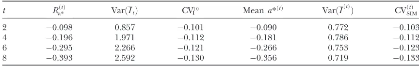
wish to mimic. Each generation,Nm¼40 males andNf¼ 160 females are randomly mated,Nf/Nm ¼4 females mated to each male. Among the 160 females (litters), 1 female from each of the 4 mated to each male is randomly chosen, so that 20 females and 20 males contribute offspring to the next generation. From each of the 20 females, 8 female offspring and 2 male offspring per female are chosen as parents of the next generation. There is no variance in the number of males or females contributed by male and female parents, giving an effective population size of 80. The number of records measured in each of the 160 females isn¼3. The index (22) is calculated for each female and the process is repeated during eight generations. There is good agreement between the empirical variance of the index obtained from 1000 replicated simulations and the variance computed from the exact formula (A8). The approximate formula (32) understates the variance in later generations. The coefficient of variation of the index increases from a value of 11.3% in generation 2 to 15.2% in generation 8 (simulation results, not shown). The corresponding values predicted by formula (34) are 10.9 and 14.9%, respectively.

The validity of the approximations to predict changes of various quantities under selection is illustrated in Table 3. Columns 2–4 refer to predictions based on formulas (23), (32), and (34). Columns 5–7 show the corresponding results obtained from 500 replications of the experiment. A similar data structure as in the

random mating situation is simulated. The number of males isNm¼40, and the total number of females isNf¼ 160 withNf/Nm¼4 females mated to each male. The index (22) was computed for each of the 160 females and the 80 best-scoring females were selected. From each of these 80 females, two daughters were chosen as mothers to produce the next generation, and one son was chosen as father from each of 40 females randomly selected among the group of 80. The effective popula-tion size calculated from the expression in Hill(1972)

is 116. This value agrees well with that derived from the simulated data based on the rate of inbreeding, despite the fact that Hill’s formula assumes no selection. The expected response in the unobservable additive genetic values affecting environmental variance (column 2) tends to overpredict the simulated results. Part of this can be attributed to the selection intensityi based on normality used in (23). For a proportion selected of 50%, a ratio of the standardized mean among selected individuals obtained from a chi-square distribution with

n1¼2 d.f. (as an approximation to the distribution of the selection criterionI) and from a normal distribu-tion is0.87 (not shown). The ratio of the simulated to the predicted response is between 0.90 and 0.92. The overprediction of formula (23) increases at higher selection intensities.

Contrary to the situation under random mating, the variance of the mean of the index computed from (32) overestimates the variance obtained from the simula-tion. Formula (32) predicts an increase due to genetic drift, but the variance falls instead. This is due to the strong scale effect between the mean and the variance of the mean index, not accounted for in the predictions. The opposite holds when selection is for higher varia-tion (not shown). The predicvaria-tions of the variance of the mean of the index corresponding to generations 2, 4, 6, and 8, computed from (35) are 0.828, 0.836, 0.815, and 0.774, which better reflect the simulated results (see Table 3). When 40 of 160 litters are selected, the results for generations 2, 4, 6, and 8 are as follows (predicted; simulated):ð0:824;0:743Þ,ð0:787;0:744Þ,ð0:709;0:714Þ, andð0:615;0:626Þ.

TABLE 2

Eight generations (t) of random mating

t VarEXACTðItÞ VarðItÞ VarSIMðItÞ

2 0.90 0.97 1.06

4 1.30 1.26 1.46

6 1.79 1.60 1.77

8 2.09 1.89 2.11

VarEXACTðItÞ, variance of indexI(Equation 22) computed

using the exact formula (47); VarðItÞ, variance ofIcomputed

using approximation (32); VarSIMðItÞ, variance ofIover 1000

replicated simulations.

TABLE 3

Observed and predicted changes under selection

t Ra*ðtÞ VarðItÞ CVI(t) Meana*ðtÞ VarðI ðtÞ

Þ CVðSIMtÞ

2 0.098 0.857 0.101 0.090 0.772 0.103

4 0.196 1.971 0.112 0.181 0.786 0.112

6 0.295 2.266 0.121 0.266 0.753 0.123

8 0.393 2.592 0.130 0.356 0.719 0.133

Ra*ðtÞ, expected response to selection ina* in generationtcomputed from approximation (23) multiplied byt; VarðItÞ, variance of the average index computed from (32); CV

ðtÞ

I , coefficient of variation computed from (34); meana*ðtÞ

, meana* at generationtover 500 replicated simulations; VarðIðtÞÞ, variance ofIin the selected line, per generation, over 500 replicated simulations; CVðSIMtÞ , coefficient of variation of the index over 500 replicated simulations.

There is good agreement between the evolution of the coefficient of variation of the mean index predicted using (34) and the simulated results (Table 3, columns 4 and 7). The agreement holds also with more intense selection (contrary to the case with the prediction of changes of the other quantities, which deteriorate with higher selection pressure). For example, with 40 females selected of 160 scored, the values of the coefficient of variation of the mean index in generations 2, 4, 6, and 8 are (predic-ted; simulated): ð0:105;0:106Þ, ð0:118;0:121Þ,

ð0:129; 0:132Þ, andð0:140;0:137Þ. Under selec-tion formula (34) for the coefficient of variaselec-tion, ignoring selection provides a good approximation.

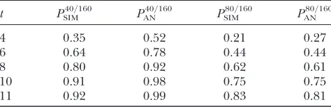
Sample size calculations:We consider the hierarchi-cal mating design described above, also with either 40 or 80 females contributing as parents of 160 scored. We envisage a situation where a fixed number of facilities per generation is available and the length of the experiment can be varied. Table 4 shows the power to detect response to selection computed using simulation and using approximation (37). Power numbers agree well at the low selection intensity but are overpredicted at the higher selection intensity. This is due to the overprediction of selection response. As shown in Table 4, to detect response to selection with 80% power and a probability of type I error of 5%, when 40ð80Þof 160 females are selected, requires an experiment spanning over 8ð11Þgenerations. As a point of reference, from formulas in Hill (1980), when 40 (80) females are

phenotypically selected from 160 scored, in the absence of a control line, detecting a response at the level of the mean with 80% power and a probability of type I error of 5% requires an experiment spanning 4ð6Þgenerations. Second, consider the length of the experiment re-quired on the basis of the Nicholas criterion. If selection is for reduced variation, with the same values of parameters, to obtain with probability 80% a response in the index that is negative (as desired), when 40ð80Þof 160 females are selected, requires an experiment spanning over 2ð3Þgenerations. To obtain a response that is 50% of the expected response with 80% proba-bility, when 40ð80Þof 160 females are selected, requires

an experiment spanning over 4 ð6Þ generations. To obtain a response that is 80% of the expected response with 80% probability, when 40 ð80Þof 160 females are selected, requires an experiment spanning over 12ð18Þ

generations.

DISCUSSION

Statistical analysis: In this work two models were compared using various criteria and the results of this exercise favor model 2 (the genetically heterogeneous environmental variance model). Several lines of evidence support this conclusion. First, the graphical assessments displayed in Figure 4 are suggestive of a negative correlation between environmental variation of litter size and genetic values for litter size. The posterior mean of the correlation coefficientrwas0.74 and the support was shifted a long way from the value of zero. Further, the Monte Carlo estimate of the 95% posterior interval of the additive genetic variance associated with the environmental variance was ð0:10;0:25Þ and the support is comfortably away from extremely small values in the vicinity of zero. The modal value of one of the priors used was 0.033, and the Monte Carlo estimate of the modal value of the posterior distribution was 0.139, indicating that the data caused the distribution to shift farther away from zero. The prior with modal value 0.300 resulted in a posterior mode of 0.141 (see Figure 1). Finally, model 2 is also supported by the deviance information criterion.

A negative correlation between genes affecting mean and variance could in principle facilitate improving litter size and simultaneously reducing its variation in repeated parities. The model postulates that genotypes that are expected to produce large litters are less likely to show departures from their expectation than genet-ically less prolific individuals. A discussion on possible mechanisms involved in the regulation of environmen-tal variation is in Falconerand Mackay(1996).

The rabbit data span 10 generations. The raw co-efficient of variation of the average index was computed each generation to search for the trend predicted by (34). However, the picture is too erratic and no clear trend could be detected.

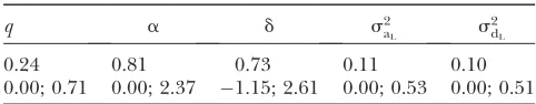
One could speculate on what other unaccounted factors could misleadingly lead to a better relative fit for model 2, even in the absence of s2

a*. Variance hetero-geneity could be caused by unaccounted major genes. To investigate whether a gene of large effect might be operating, a segregation analysis was performed, fitting a Bayesian–MCMC model similar to model 1 with the addition of one putative major locus. This mixed in-heritance model is described in Sorensenand Gianola

(2002, pp. 672–679), where full details can be found. The parameters associated with the major locus are the initial gene frequency, q, the additive ðaÞ and dominanceðdÞdeviations, the additive and dominance TABLE 4

Evolution of power across generations (t) to detect response to selection for reduced variance with two selection intensities

t PSIM40=160 P 40=160

AN P

80=160

SIM P

80=160 AN

4 0.35 0.52 0.21 0.27

6 0.64 0.78 0.44 0.44

8 0.80 0.92 0.62 0.61

10 0.91 0.98 0.75 0.75

11 0.92 0.99 0.83 0.81

PSIM40=160, power obtained using simulation (40 litters selected of 160); PAN40=160, power computed analytically using (37); PSIM80=160 andP

80=160

genetic variances associated with the major locus

ðs2 aL;s

2

dLÞ, and their sum ðs 2

GLÞ. The posterior means for these quantities and 95% posterior intervals are shown in Table 5. Given the model, the results show that litter size is affected by a recessive gene whose frequency at the start of the experiment is low ð0:24Þand whose contribution in terms ofs2

aLands 2

GLrelative to the total phenotypic variance for litter size is 0.020 and 0.038, respectively. Relative to the total genetic variance (sum of the polygenic component and the total major locus genetic variance), these numbers are 0.16 and 0.30. The recessive homozygote genotype decreases litter size by 0.81 kits, and the heterozygote genotype increases it by 0.73 kits (based on estimated posterior means in Table 5). The 95% posterior intervals indicate that there is very large posterior uncertainty associated with these inferences. The Monte Carlo estimate of the DIC for this model is 7825. The estimated DIC corresponding to model 1 is 7810, which reveals that the data do not provide support for the presence of a major locus. This is consistent with the amount of posterior uncertainty (see the 95% posterior intervals in Table 5).

The segregation analysis was fitted as an extension of model 1 only. The amount of variation contributed by the major locus (total genetic variance) is at a theoret-ical maximum in those groups of individuals where the gene frequency is 0.70, and it does not contribute when the gene is fixed or lost. Using the estimates of posterior means from Table 5, the maximum possible contribu-tion is 0.60. The range of within-group variacontribu-tion in Figure 4A is from 2.4 to 3.9. More precisely, the largest and smallest values for the environmental variance estimated fitting model 2 are 2.83 and 6.99, respectively. Further, we computed the gene frequency of the re-cessive allele in each of the groups in Figure 4A, and it fluctuated around 0.30 with no detectable association with within-individual variation across groups. We con-clude that the variance heterogeneity postulated by model 2 cannot be explained by an unaccounted effect of the major locus only. Under the mixed-inheritance model, our results are in very good agreement with those reported by Argente et al. (2003) who used a

similar data set. However, Argenteet al. (2003) fitted a

mixed-inheritance model only and based their

conclu-sions on this single model. The analysis reported here based on the mixed-inheritance model agrees with theirs, but the DIC favors model 1.

Selection for environmental variation: Attempts to show the existence of genetic heterogeneity of environ-mental variance analyzing field or experienviron-mental data that have not been specifically collected to address this issue provide circumstantial support for the model. One can never rule out artifacts, such as confounding between genetic and environmental effects, the scale of measurement, or the existence of a hidden mixture due to disease, say, that would favor the genetically heterogeneous environmental variance model relative to the other models. For example, if the distribution of the data is skewed in either direction, the genetically heterogeneous environmental model would fit rela-tively better than the standard model, yielding a co-efficient of correlation between the additive genetic values affecting mean and variance whose sign and magnitude would depend on the direction and degree of skewness (Ros et al. 2004). Another source of

spurious results could be due to the wrong choice of functional relationship between mean and variance postulated by the model (Ros et al. 2004). Some but

certainly not all of these limitations can be overcome if the evidence comes not from fitting the model, but rather from using simple functions of the data whose pattern would be consistent with the presence of genetic effects on the variance. Figure 4A is an example. A more sophisticated approach in this spirit is in Rowe et al.

(2006), who found evidence for genetic variance in environmental variance, analyzing the variance of the variance of large half-sib families for juvenile growth in broiler chickens.

On the other hand, a selection experiment showing that the environmental variance responds to selection would provide strong evidence. Such an experiment poses chal-lenges in terms of number of individuals, design, criterion of selection, and the analysis and evaluation of response. Here we attempted to address some of these issues, with special emphasis on the size of the experiment.

The predictions of the evolution of the mean of genetic values affecting the variance and of the mean index deteriorate as selection intensity becomes more intense. We have also studied selection at the level of lnI, which, using the delta method, can be shown to be asymptotically normally distributed with mean b* and variance equal tos2

a*12=ðn1Þ. The mean and vari-ance of lnIjb*,a* areb*1a* and 2/(n1), respectively, mutually independent. Standard normal theory can then be used, which leads to simple algebra. For example, the expected response ina* and in lnIwhen selection is based on ln I is is2

a*=

ffiffiffiffiffiffiffiffiffiffiffiffiffiffiffiffiffiffiffiffiffiffiffiffiffiffiffiffiffiffiffiffi

s2

a*12=ðn1Þ p

, approximately the same as (23) ifs2

a*is small andnlarge (selecting onIor on lnIshould lead to the same choice of parents), but different from (27). The variance of the mean lnI equivalent to (32) iss2

a*=m12=mðn1Þ1 TABLE 5

Monte Carlo estimates of posterior means (first row) and of 95% posterior intervals (second row) of parameters

from the segregation analysis model

q a d s2

aL s

2 dL

0.24 0.81 0.73 0.11 0.10

0.00; 0.71 0.00; 2.37 1.15; 2.61 0.00; 0.53 0.00; 0.51

q, gene frequency of a recessive allele;a, additive deviation;

d, dominance deviation;s2

aL, additive genetic variance at a

ma-jor locus;s2

dL, dominance variance at a major locus.

ðt=NÞs2

a*. There is an appealing simplicity in these expressions that are independent ofb*. Unfortunately, with typical values ofn3 or 4 the approximation based on the delta method does not perform well, especially when several generations of selection are involved.

An alternative model of genetically structured envi-ronmental variance was postulated by Hilland Zhang

(2004) and Mulderet al. (2007, 2008). In their model,

the phenotype is assumed to be conditionally nor-mally distributed (given genotype), with the same mean as in (21), and with conditional variance equal to expðb*Þ1a*, rather than expðb*Þexpða*Þ as in (21). In the case of our model, as mentioned in Sorensen

and Waagepetersen(2003),

expða*Þ ¼exp arsa*

sa

1u

;

whereu¼a*Eða*jaÞisN 0;s2 a*ð1r

2_Þ

, indepen-dent of a. Thus our model postulates a stochastic relationship between the mean and the log-variance. When the components of the argument of the expo-nential of the right-hand side are small,

exp arsa*

sa

1u

11arsa*

sa

1u;

so the mean–variance relationship is approximately linear. The Mulderet al. (2007, 2008) model assumes

a linear stochastic relationship between the mean and the variance. There is thus little difference in this feature between the models when aðrsa*=saÞ1u is small. Other functional relationships could be con-ceived, with noa priorimechanistic justification for the choice. A rationale for this choice could be based on a posterior analysis. In both of these models, the marginal distribution of phenotype is unknown. The mean of the marginal distribution of phenotype is the same in both models but the marginal variance under the model of Mulder et al. (2007, 2008) is expðb*Þ1s2

a, as in the homogeneous variance model. The focus in Mulder et al. (2007, 2008) is to derive expressions to predict changes inða;a*Þafter one cycle of selection on the basis of either phenotype or an index, but not on the evalua-tion of these changes. Under their model, the condi-tional expectation of the index, givena*, is

EðIjb*;a*Þ ¼expðb*Þ1a*;

and the expected change in the index (22) due to the expected change ina*, equivalent to expression (27), is

Esða*Þ, not dependent on b* [this expectation is different from (23)]. However, it can be shown that the termRIðtÞ=

ffiffiffiffiffiffiffiffi

VðtÞ

p

, which features in the determina-tion of size of experiment, depends on expðb*Þ. We have not found that the types of computations carried out in this study are simpler under this alternative model.

This work has centered exclusively on describing a simple approach to reduce environmental variation by

selection and to measure this reduction, as a means of validating the genetically heterogeneous environmental variance model. No attention was given to the correlated change in mean, a subject studied in detail in the work of Mulderet al.(2007, 2008). In a typical selection program

in cases where a near optimum for the mean has been approached, one may be interested in increasing relative selection pressure on the variance (Mulderet al.2008).

This leaves a proportionð1r2_{Þof the variances}2 a* to manipulate environmental variation by selection. Clearly, in such a situation a relatively larger experiment would be needed to detect selection response in variance.

LITERATURE CITED

Argente, M., M. Santacreu, A. Climent, G. Boletand A. Blasco, 1997 Divergent selection for uterine capacity in rabbits. J. Anim. Sci.75:2350–2354.

Argente_{, M. J., A. B}lasco_{, J. A. O}rtega_{, C. S. H}aley_{and P. M.} Visscher, 2003 Analyses for the presence of a major gene af-fecting uterine capacity in unilaterally ovariectomized rabbits. Genetics163:1061–1068.

Besag, J., 1974 Spatial interaction and the statistical analysis of lat-tice systems (with discussion). J. R. Stat. Soc. Ser. B36:192–236. Falconer, D. S., and T. F. C. Mackay, 1996 _{Introduction to}

Quantita-tive Genetics.Longman, New York.

Garcı´a, M. L., and M. Baselga, 2002 Estimation of genetic re-sponse to selection in litter size using a cryopreserved control population. Livest. Prod. Sci.74:45–53.

Gavrilets_{, S., and A. H}astings_{, 1994 A quantitative genetic model} for selection on developmental noise. Evolution48:1478–1486. Gelfand_{, A. E., 1996 Model determination using sampling-based} methods, pp. 145–161 inMarkov Chain Monte Carlo in Practice, edi-ted by W. R. Gilks, S. Richardsonand D. J. Spiegelhalter. Chapman & Hall, London/New York.

Gelfand, A. E., D. K. Deyand H. Chang, 1992 Model determina-tion using predictive distribudetermina-tions with implementadetermina-tion via sam-pling-based methods, pp. 147–167 inBayesian Statistics 4, edited by J. M. Bernardo_{, J. O. B}erger_{, A. P. D}awid_{and A. F. M. S}mith_. Oxford University Press, London/New York/Oxford.

Gelfand_{, A. E., S. K. S}ahu_{and B. P. C}arlin_{, 1996 Efficient} param-eterizations for generalized linear mixed models, pp. 165–180 in Bayesian Statistics 5, edited by J. M. Bernardo, J. O. Berger, A. P. Dawid_{and A. F. M. S}mith_{. Oxford University Press, London/} New York/Oxford.

Gelman_{, A., J. B. C}arlin_{, H. S. S}tern_{and D. B. R}ubin_{, 1995 Bayesian} Data Analysis.Chapman & Hall, London/New York.

Gelman_{, A., X. L. M}eng_{and H. S}tern_{, 1996 Posterior predictive} assessment of model fitness via realized discrepancies (with dis-cussion). Stat. Sin.6:733–807.

Gutierrez, J. P., B. Nieto, P. Piqueras, N. Iba´ n˜ ezand C. Salgado, 2006 Genetic parameters for canalisation analysis of litter size and litter weight at birth in mice. Genet. Sel. Evol.38:445–462. Hill, W. G., 1972 Effective size of populations with overlapping

gen-erations. Theor. Popul. Biol.3:278–289.

Hill, W. G., 1980 Design of quantitative genetic selection experi-ments, pp. 1–13 inSelection Experiments in Laboratory and Domestic Animals, edited by A. Robertson. Commonwealth Agricultural Bureaux, Slough, UK.

Hill, W. G., and X. S. Zhang, 2004 Effects on phenotypic variability of directional selection arising through genetic differences in re-sidual variability. Genet. Res.83:121–132.

Iba´ n˜ ez, N., L. Varona, D. Sorensenand J. L. Noguera, 2007 A study of heterogeneity of environmental variance for slaughter weight in pigs. Animal2:19–26.

Little_{, R. J. A., and D. B. R}ubin_{, 1987 Statistical Analysis with Missing} Data.Wiley, New York.