ADAMS, BRIAN MICHAEL. Non-parametric Parameter Estimation and Clinical
Data Fitting with a Model of HIV Infection. (Under the direction of H. Thomas
Banks.)
The focus of this dissertation is to develop a combined mathematical and statistical
modeling approach for analyzing clinical data from an HIV acute infection study. We
amalgamate two existing models from the literature to create a nonlinear differential
equation model of in-host infection dynamics that is capable of predicting sustained
low-level viral loads and multiple stable equilibria. Using this example system of
dif-ferential equations we demonstrate two contrasting parameter identification problem
formulations for estimating the distribution of model parameters across a population:
the first at the individual patient level and the second directly at the population level
itself. In the latter case one leverages data from all patients to estimate a
proba-bility density function representing the distribution. We discuss well-posedness and
computational implementation for such inverse problems. Directly estimating the
dis-tribution in this way may offer computational advantages over estimating parameters
for individual patients.
In the context of the model, we implement the Expectation Maximization (EM)
Algorithm for maximum likelihood estimation to handle patient measurements
on the knowledge that they are censored. In addition, in both inverse problem
con-texts (estimating a vector of parameters for a single patient and the distribution of
a parameter across all patients) we develop and apply methods for estimating
vari-ability of the resulting parameter estimates by using sensitivity analysis to calculate
confidence intervals.
We validate each of the methods with simulated data and demonstrate typical
results. Finally we present results for the application of the methods to actual clinical
data and give examples of conclusions that one might draw from them. This model
fitting approach may help clinicians better understand patient behaviors and notably,
could alert them to the expected long-term trend for a particular patient.
Brian Michael Adams, born October 10, 1977, in Bridgeport, Connecticut, grew up in
the rural Vermont towns of Underhill and Jeffersonville. He was primarily educated
in the public schools of those towns including Lamoille Union High School, where his
love of science and mathematics became evident and interests in technical theatre and
music flourished. Community and family experiences complemented his traditional
academic learning. Through Scouting, working in a local hardware store, and assisting
his parents in restoring a late 1800s farmhouse, he developed skills and sensibilities
he values immensely to this day. He graduated Salutatorian from Lamoille Union
in June 1995, and, not feeling too geographically adventurous, chose to attend Saint
Michael’s College in Colchester, Vermont.
Some have suggested that Brian’s undergraduate career consisted mainly of
learn-ing about and playlearn-ing music, supportlearn-ing the campus computlearn-ing community as a
sys-tems and network specialist, participating in church activities and community service
projects, and engineering live sound for concerts. While the author does not refute
these allegations, he did spend considerable time studying mathematics, computer
science and humanities. Brian earned a Bachelor of Science degree in Mathematics
with minors in both Music and Computer Science and certification to teach secondary
school mathematics. He graduated Valedictorian in May 1999, mathematically richer,
significantly more aware of cultural and social justice concerns, and desiring to
volunteer in New Orleans, Louisiana, teaching inner-city middle schoolers religion and
computer skills. He concurrently installed a data, voice, and video network that he
would maintain for four more years. Aware that a lifetime in the Crescent City was
not for him, Brian next tried to satiate his curiosity as to how he could utilize all the
previously-learned mathematics.
In Summer 2000 the author settled in Raleigh, NC, where he quickly learned
about living in a bigger city and to appreciate cooking and eating good food and
traveling to various places for conferences. His graduate career started at North
Car-olina State University with the support of a U.S. Department of Education GAANN
Computational Science Fellowship. After completing initial coursework in applied
mathematics and a summer internship at Fred Hutchinson Cancer Research Center,
he received his Master’s degree in December 2000. Delighted to be more aware of the
various uses of mathematics and compelled to study biological applications, Brian
continued research in mathematical biology under the direction and support of Dr.
H.T. Banks. Dr. Banks advised him on a minor project on population models for
aphids, and then through completion of his Ph.D. project on modeling HIV infection
in Summer 2005. He earned a Ph.D. in Computational and Applied Mathematics to
be awarded December 2005.
Brian has accepted a research position at Sandia National Laboratories in
Albu-querque, New Mexico. He looks forward to the adventures that await him there.
Many extraordinary people influenced my growth through course work and research
collaboration at NC State. Since recruiting me to the applied math program five
years ago, Dr. H.T. Banks has served as my teacher, research advisor, and mentor.
He exposed me to the breadth of mathematics and sciences through classes, personal
dialog, and conference travel, and helped me settle on research in math biology. Dr.
Banks took an interest in my mathematical and personal pursuits and, at crucial
times, reminded me of the importance of balance between the two. I am grateful for
his selfless commitment to our work and constant encouragement and support.
The members of my advisory committee have played important roles as well; I
appreciate the classes they each taught and time they spent discussing my research.
Dr. Hien Tran taught an excellent class in mathematical modeling and shared in
lengthy discussions on our HIV model and biological modeling and control in general.
Dr. Marie Davidian spent hours meeting and preparing notes to help me understand
statistical concerns and approaches. Two classes and a qualifying examination with
Dr. Bob Martin convinced me of the beauty of functional analysis. He clarified
anal-ysis details in this dissertation and mentored me in the Preparing the Professoriate
program.
Numerous others contributed to the HIV modeling project. I initially learned
about HIV infection pathways and current related mathematical research with the
working and living there a joy. More recent collaborations have been with Shannon
Wynne, Yanyuan Ma, Hee-dae Kwon, Jari Toivanen, Shuhua Hu, and Sarah Grove.
I thank Grace Kepler for helpful discussions and candid advice, and Eric Rosenberg
for providing clinical data and sharing in discussions on HIV immunology.
This work would not be possible without mathematical foundations and I am
grateful to the professors who have influenced me over the years. Professors in the
St. Michael’s College mathematics department were instrumental in starting me in
this field. At NC State, Tim Kelley and Michael Shearer particularly influenced me
through their courses. For mathematical, personal, and computer-related discussions,
especially early-on in graduate school, I thank fellow students Brian Ball, Kristy
Coffey, Todd Coffey, Nathan Gibson, Katie (Kavanagh) Fowler, Rachel Levy, Brian
Lewis, Jordan Massad, Jim Nealis, and Bob Wieman. The staff in our department has
been wonderfully supportive; Rory Schnell and Brenda Currin in particular helped
me through administrative hassles and listened patiently many times.
My friends and family have kept me focused on my work and helped me relax
when necessary. Long-term friends from high school and college, especially Adam
Kropelin, Susan Hebert, and Casey Reever supported me at various stages of the
process. Here in Raleigh I recognize all my (also mathematical) friends, including
Jason Osborne, Jill Reese, Jeremy Scott, Brandy Benedict (including for suggestions
on this manuscript), and Teresa Selee. The many people with whom I have played
music over the years deserve special recognition for helping preserve my sanity.
Fi-nally, huge thanks go to my eternally supportive and encouraging parents, Carl and
Barbara Adams.
My graduate studies, including this research, have been supported financially
lowship program. This dissertation work was also supported in part by the Joint
DMS/NIGMS Initiative to Support Research in the Area of Mathematical Biology
under grant 1R01GM67299-01, and benefited from facilities at the Statistical and
Applied Mathematical Sciences Institute, which is funded by NSF under grant
DMS-0112069.
List of Tables ix
List of Figures xi
Notation xv
1 Introduction 1
2 Clinical Data and Desired Outcomes 5
3 Mathematical Models for HIV Infection 15
3.1 Survey of Existing Models . . . 15
3.2 Proposed Model: Features and Analysis . . . 18
3.2.1 Sample model parameters, steady states, and treatment efficacy 27
3.2.2 Existence and computation of model solution . . . 37
3.3 Error Model and Simulated Data . . . 44
3.4 Sensitivity Computations . . . 47
4 Parameter Identification (Inverse) Problem 54
4.1 Inverse Problem Formulations . . . 55
4.2 Analysis of Inverse Problems . . . 62
4.2.3 Existence of a minimizer and method stability . . . 67
4.3 Statistical Theory and Methods . . . 71
4.3.1 Confidence intervals . . . 71
4.3.2 Censored data methodology . . . 77
4.4 Computational Methods . . . 81
5 Method Validation with Simulated Data 83 5.1 Estimation of PDFs and Confidence Bands . . . 83
5.1.1 Uniform simulated cohort . . . 87
5.1.2 Treatment-varied simulated cohort . . . 95
5.1.3 Dynamics-varied simulated cohort . . . 100
5.1.4 Confidence intervals . . . 102
5.2 Testing of Censored Data Methods . . . 105
6 Model Fitting to Clinical Data 119 6.1 Fits to Individual Patients . . . 119
6.2 Estimation of Distributions . . . 134
7 Conclusions and Future Directions 141
References 144
A Model Fits to Clinical Data 149
2.1 Summary of patient data . . . 10
2.2 Patients in various ranges of off treatment time. . . 13
3.1 State variables used in HIV model . . . 21
3.2 Dynamic parameters used in HIV model . . . 28
3.3 Off treatment model steady states . . . 31
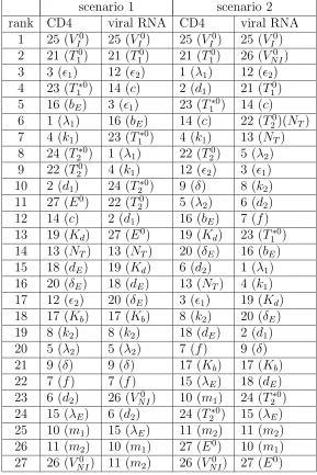
3.4 Semi-relative sensitivities of CD4 and viral RNA with respect to each of 27 parameters in two scenarios. . . 52
3.5 Parameters ranked by semi-relative sensitivity for CD4 and viral RNA in two scenarios. . . 53
5.1 Ranges prescribed for generating distributions of parameters. . . 86
5.2 Influence of regularization on conditioning in quadratic programming problem. . . 89
5.3 Results for censored data algorithm ¯σ= 0.2 . . . 108
5.4 Results for censored data algorithm ¯σ= 0.3 . . . 110
5.5 Simulated censored data: sample parameter estimates and standard errors . . . 118
6.1 Bounds employed when estimating parameters from clinical data. . . 120
6.3 Clinical data: estimated parameters and standard errors for Patients
1–30 . . . 124
6.4 Clinical data: estimated parameters and standard errors for Patients
31–59 . . . 125
6.5 Clinical data: estimated parameters and standard errors for Patients
31–59 . . . 126
6.6 Summary statistics for clinical data with censored data algorithm. . . 127
6.7 Calculated model equilibria given each patient’s estimated parameters,
patients 1–30. . . 129
6.8 Calculated model equilibria given each patient’s estimated parameters,
patients 31–59. . . 130
2.1 Treatment protocols for patients 1–59 . . . 11
2.2 Treatment protocols for patients 60–118 . . . 12
2.3 Frequency plots: percentage time off treatment. . . 13
2.4 Sample CD4+ T-cell and censored viral load data. . . . 14
3.1 Schematic of compartmental HIV infection dynamics model. . . 21
3.2 Sample control input (treatment protocol) u(t) representing STI. . . . 23
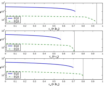
3.3 Sensitivity of viral load equilibria to drug efficacy ǫ1 . . . 33
3.4 Sensitivity of viral load equilibria to drug efficacy ǫ2 . . . 34
3.5 Sensitivity of viral load equilibria to drug efficacies ǫ1, ǫ2 . . . 35
3.6 Regions of stability for equilibria given various values of treatment efficacies ǫ1 and ǫ2. . . 36
3.7 Simulation of early infection scenario using HIV model . . . 43
4.1 Example of piecewise linear spline approximation to density function f(q). . . 59
4.2 spline approximation to density functionf(q) with confidence intervals 74 5.1 Sample normal and bimodal densities f on log10(q)∈[−1,1]. . . 87
5.2 Uniform simulated cohort: estimated normal p.d.f. of k1, NS = 8, various NP. . . 88
P
5.4 Uniform simulated cohort: estimated normal p.d.f. of k1, NP = 1024,
various NS. . . 90
5.5 Uniform simulated cohort: estimated bimodal p.d.f. ofk1,NP = 1024,
various NS. . . 91
5.6 Uniform simulated cohort: estimated normal p.d.f. of k1, NP = 1024,
various NS with regularization. . . 91
5.7 Uniform simulated cohort: estimated bimodal p.d.f. ofk1,NP = 1024,
various NS with regularization. . . 92
5.8 Influence ofβR on estimated p.d.f. in normal case. . . 92
5.9 Uniform simulated cohort: estimated p.d.f.s of d1, NP = 64, NS = 16,
with regularization. . . 93
5.10 Uniform simulated cohort: estimated p.d.f.s ofNT,NP = 64, NS = 16,
with regularization. . . 93
5.11 Uniform simulated cohort: estimated p.d.f.s of c, NP = 64, NS = 16,
with regularization. . . 94
5.12 Treatment-varied simulated cohort: estimated bimodal p.d.f. of k1,
NS = 8, various NP. . . 95
5.13 Treatment-varied simulated cohort: estimated bimodal p.d.f. of k1,
NS = 16, various NP. . . 96
5.14 Sample normal and adjusted bimodal distributions for d1. . . 97
5.15 Treatment-varied simulated cohort: Fitting bimodal p.d.f. when
ex-pected value is close to that of normal, NS=8 . . . 98
5.16 Treatment-varied simulated cohort: Fitting bimodal p.d.f. when
ex-pected value is close to that of normal, NS=16 . . . 99
5.18 Uniform simulated cohort: Confidence intervals for estimates of normal
distribution ofk1, withNS = 4,8,16; βR= 0 . . . 102
5.19 Uniform simulated cohort: Confidence intervals for estimates of normal distribution ofk1, withNS = 4,8,16; βR= 0.01 . . . 103
5.20 Uniform simulated cohort: Confidence intervals for estimates of bi-modal distribution of k1, with NS = 4,8,16; βR= 0.0001. . . 103
5.21 Uniform simulated cohort: Confidence intervals for estimates of normal and bimodal distribution ofd1, withNS = 16; βR = 0.01 . . . 104
5.22 Sample fit to simulated censored data (¯σ = 0.2) with censored data algorithm for fourth parameter set with initial iterate 1.05q0. . . 113
5.23 Sample fit to simulated censored data (¯σ = 0.2) with censored data algorithm for seventh parameter set with initial iterate 0.90q0. . . 114
5.24 Sample fit to simulated censored data (¯σ = 0.2) with censored data algorithm for seventh parameter set with initial iterate 1.01q0. . . 115
5.25 Sample fit to simulated censored data (¯σ = 0.2) with censored data algorithm for sixth parameter set with initial iterate 0.90q0. . . . 116
5.26 Loglikelihood vs. iteration for parameter set 2 . . . 117
5.27 Loglikelihood vs. iteration for parameter set 2 . . . 117
6.1 Sample model fit for patient 5 . . . 121
6.2 Sample model fit for patient 5 – all model states . . . 131
6.3 Sample model fit for patient 8 . . . 132
6.4 Sample model fit for patient 8 – all model states . . . 133
6.6 Distribution of estimated parameters and estimated piecewise linear
density . . . 137
6.7 Schematics of initial iterates for density functions. . . 138
6.8 Distribution of estimated parameters and estimated piecewise linear
density . . . 139
6.9 Distribution of estimated parameters and estimated piecewise linear
density . . . 140
Model State Variables and Data
ODE model state vector (unscaled) x¯
ODE model state vector (log10 scaled) x
state observer matrix∈Rm×n O
observed unscaled state vector z¯
observed log10 scaled state vector z
data (unscaled clinical or simulated) y¯
data (log10 scaled clinical or simulated) y, w
time (days) t (or tij
s)
parameter vector q
fixed parameters q`
differential equation dynamics g(t, x;q), h(t, x;q)
assay censor limits (unscaled) L¯1,L¯2
assay censor limits (log-scaled) L, L1, L2
Dimensions
size of full ODE model state vector n
size of observed ODE model state vector m
number of time points (possibly patient-dependent) N (or Nj, Nj s)
number of patients NP
number of spline intervals NS
dimension of estimated parameter vector p
Indices
time point index i
patient index j
spline indices k, l
state vector index s
standard error ν
variance σ2
covariance matrix Σ
cumulative distribution function F(q)
probability density function f(q)
set of functions F
a probability distribution P
probability space (set of distributions) P
expected value E
matrix operator for expected value E
indicator function χ
likelihood function L
Other
spline “hat” basis function φk(q)
spline coefficients dk
spline knots qk
Jacobian matrix J
cost criterion J
regularization parameter βR
rational numbers Q
natural numbers {1,2,3, . . .} N
• Optimal estimates resulting from parameter estimation procedures will be de-noted by (ˆ·) or (·)∗
.
• u(t) denotes a control input (treatment function), which we assume has a piece-wise linear form and so is specified by times when treatment changes.
Introduction
Human Immunodeficiency Virus (HIV) is a retrovirus that infects T-helper cells of the
immune system and is the causative agent for Acquired Immune Deficiency Syndrome
(AIDS). HIV and AIDS are among the world’s most serious public health concerns,
affecting people of all demographics worldwide, with some regions impacted
dispro-portionately. As of 2003, an estimated 38 million HIV-infected individuals are living
worldwide, with approximately two-thirds in Africa, where 2.2 million people died
from opportunistic infections related to AIDS in 2003 (UNAIDS 2004 Report on the
Global HIV/AIDS Epidemic [3]).
Despite many successful public health and clinical interventions since the first
iden-tification of HIV-positive patients in 1981, there remains no cure and the HIV/AIDS
epidemic continues to grow. In 2003, 4.8 million people became newly infected with
HIV, with over half of new cases occurring in youth ages 15–24. This is despite the fact
that effective transmission prevention strategies exist. A possible factor for continued
spread in industrialized countries is behavior resulting from the myth that
antiretro-viral drugs, which often successfully suppress virus and improve patient quality of life,
constitute a cure for HIV infection. Infection rates continue to rise around the world,
with the fastest expansions of the epidemic occurring in Asia and Eastern Europe.
Thus, developing effective methods for prevention of transmission and related public
health education campaigns remains crucial.
While antiretroviral drugs are widely available in the United States and Western
Europe, their cost and side effects may make their use challenging. In developing
nations, UNAIDS estimates that only 7% of the infected population has access to
antiretroviral drugs. Access to treatment for and education about this disease remain
serious human rights issues around the world. In all geographies, ever-improving
strategies are needed for efficient and appropriate use of drug therapy.
The epidemiology of HIV and public health issues like transmission (inter-host
dy-namics) are important to study. As important to investigate are the effective use and
improvement of antiretroviral drugs, which depend on understanding viral behavior
within each host, including pathways of infection and effects of drugs. Understanding
intra-host viral and immune system pathways depends on knowledge from various
biological areas including physiology and immunology. Mathematical models can aid
in quantifying dynamic physiologic and immunologic processes and correlating the
scientific knowledge of these processes with observed patient behavior.
It is believed that the acute and early phases of HIV infection provide crucial
in-formation about immune responses and viral dynamics. In particular, long-term viral
set points and speed of progression to AIDS may possibly be understood by studying
these key periods. Motivated by clinical study data from patients observed during
the crucial acute infection phase and beyond, we develop a combined mathematical
and statistical approach to modeling HIV infection in this dissertation. We use both
simulated (virtual) data and clinical data to demonstrate the methods and kinds of
conclusions one may draw from them.
Some of these drug holidays were unprescribed or single interruptions, while others
were structured treatment interruptions (STIs) according to a study protocol. STIs
are being explored as an alternative to continuous therapy with antiretrovirals and
in addition to offering the benefit of reduced side effects may also serve to boost
HIV-specific immune responses. We therefore incorporate STI protocols in our
math-ematical models. A good overview of the concept of STI and its applicability in
various phases of HIV infection can be found in [35].
In Chapter 2 we overview the clinical acute HIV infection study and the methods
used to gather the data analyzed in this dissertation. We describe the characteristics
of the data set, including the treatment regimens undergone by various patients, and
set goals for understanding it.
Chapter 3 begins with a survey of mathematical models of in-host HIV infection
dynamics and illustrates the various disease features and pathways one might wish to
model. We then describe the particular system of differential equations used to model
HIV infection in our work and discuss its properties and solvability. We present a
statistical model to describe the relationship between the differential equation model
and the observed data and explain how it will be used to generate simulated data.
Finally, we use sensitivity equations to determine which dynamic parameters most
influence model solutions and to compute confidence intervals on parameter estimates.
In Chapter 4 we present two contrasting approaches to inverse problems with
multiple longitudinal data sets, including one in which the distribution of model
pa-rameters across the population is determined directly. Theory for well-posedness of
this method is then presented. We explain the statistical methods used to construct
confidence intervals from the sensitivity equations and the Expectation Maximization
Algorithm used to handle patient data below the limit of measurement detection. We
the parameter identification problems. The inverse problem for a distribution
pre-sented in Chapter 4 can offer substantial computational advantage over estimating
parameters individually for each patient in a data set or over more complex
hierar-chical methods where parameters and distribution parameters are estimated for each
patient.
Before applying the mathematical methods to clinical data, we test them on
sim-ulated data designed to represent the clinical data sets. In Chapter 5 we present
results of these experiments and discuss some of the strengths and weaknesses of the
censored data and probability distribution estimation methods.
Following the exploration with simulated data, we examine results for applying
the methods to clinical data in Chapter 6. Model fitting results can offer surprising
insight into patient behavior – we discuss examples here. To conclude the dissertation,
in Chapter 7 we summarize key results and offer pointers to issues requiring further
Clinical Data and Desired
Outcomes
The data for our study come from over 100 adults with symptomatic acute or early
HIV-1 infection. These subjects were enrolled in a study based at Massachusetts
General Hospital and associated regional centers and followed for varying lengths
of time between 1996 and 2004. The study cohort is unique in that its members
were all identified soon after initial infection, making its data particularly useful for
understanding early viral dynamics and related immune responses. A principal goal
of the clinical study is to assess the potential immunologic consequences of early
treatment initiation, including preservation of HIV-specific CD4+ T-cells, extent of
latent reservoir development, and homogeneity of viral population. The researchers
strive to understand the role of early immune responses in long-term viral suppression.
Clinical and demographic data were collected at the time of study enrollment and
blood draw assays of CD4+ T-lymphocyte count and RNA viral load performed at
roughly monthly follow-up visits. Viral load was quantified with Reverse
Transcriptase-Polymerase Chain Reaction (RT-PCR) methods using the commercially available
HIV-1 Roche Amplicor or Chiron Quantiplex assay, yielding measurements in viral
RNA copies per milliliter (ml). The standard assay has a linear range of 400 to
750,000 copies/ml, while the ultra-sensitive assay, 50 to 100,000 copies/ml. The
lat-ter is typically employed when a measurement is below the 400 copies/ml limit of
the standard assay, as is often the case for a patient successfully suppressing virus.
Standard flow cytometry methods were employed to obtain total plasma CD4+
T-lymphocyte counts per microliter (µl) [32].
Nearly all subjects in the study underwent combination therapy with three or more
antiretroviral drugs, although the precise regimen varied from patient to patient as
dictated by the treating physician. Fourteen of the subjects underwent structured
treatment interruptions according to a study protocol, including patients with
iden-tification numbers 2, 4, 5, 6, 10, 13, 14, and 16 for whom immune responses were
assessed during interruption [48]. Several others simply discontinued drugs at various
points. Table 2.1 summarizes the data for all 118 patients in the data set, including
the clinical identification number assigned to the patient, number of longitudinal
vi-ral load and CD4+ measurements, the total length of time from presentation to last
observation, total number of days on and off treatment, and the number of periods
(of any length) the patient was off and on therapy. Blank entries indicate patients
for whom there were no observations. The number of treatment interruptions varies
drastically over the population and some patient records include an initial brief
off-treatment phase after presentation, but before therapy commenced. In some cases,
the sum of days on and days off exceeds the total days. This is because total days
indicates the time from the start of study to last measurement of viral load or CD4
count; for some patients, data indicating treatment status extends beyond this period.
The treatment protocols and overall length of observation for each of the 118
these schematics, thicker lines denote on-treatment periods and the thinner lines,
off-treatment. The seventeen patients with no markers had fewer than two measurements
and will not be considered in our work. Since we fit a complex dynamic model to
these data, we restrict attention to the 59 patients with at least ten viral load and ten
CD4 measurements (the patients marked with an asterisk in Table 2.1) and denote
this set of patients by PS59.
The distribution of percentage of time spent off treatment by patients in PS59
is shown by histograms in Figure 2.3. The left panel includes frequency for all 59
patients, while the right panel focuses on the 28 patients who spent 10–90% time off
treatment. The total number of patients in each range is summarized in Table 2.2.
A total of 39 patients spend less than 20% time on drug holiday, with 31 spending
less than 10% time on holiday.
Some aspects of the mathematical model later considered are more readily
val-idated in the context of treatment protocols with a balance between time on and
time off treatment. Therefore, to validate mathematical methods, we later consider
the treatment schedules and observation times of patients spending 30–70% time off
treatment. This set of eighteen patients consists of those numbered 2, 4, 5, 6, 9, 10,
13, 14, 15, 16, 23, 24, 26, 27, 33, 46, 47, and 76, and we denote it by PS18. The
members of PS18 each have at least fourteen measurements per state and they will
serve as model or virtual patients for algorithm testing when we generate simulated
data based on their schedules and observation times.
Due to the linear range limits described above, the clinical viral load assays
ef-fectively have lower and upper limits of quantification. The upper limit is typically
readily handled by repeatedly diluting the sample until the resulting viral load
mea-surement is in range and then scaling. The lower limit, or left censor point, however,
lower limit of detection), the only available knowledge is that the true measurement
is between zero and the limit of detection ¯L⋆ for the assay. Those at hand have two
limits of detection, ¯L1 = 400 copies/ml for the standard and ¯L2 = 50 copies/ml for
the ultra-sensitive assay. These are illustrated in sample data shown in Figure 2.4,
where censored data points are those appearing identically on the drawn censor lines
¯
L1 = 400,L¯2 = 50. A statistical methodology for handling this type of censored data
is described later in Section 4.3.2.
The observation times and intervals vary substantially between patients. The
sample data in Figure 2.4 also reveal that observations of viral load and CD4 may
not have been made at the same time points, so in general for patient number j we
have CD4+ T-cell data pairs (tij 1, y
ij
1 ), i = 1, . . . , N j
1 and (potentially different) viral
RNA data pairs (tij2, yij2), i= 1, . . . , N2j.
We have several goals for working with this clinical data:
1. Describe the data with a mathematical model of time-varying infection
dy-namics. Leverage data to calibrate the model by estimating model dynamic
parameters. Determine if the model can predict long-term T-cell preservation
versus decline.
2. Use the data-calibrated model to extrapolate beyond the observation period to
determine consequences of various treatment schemes.
3. Use the calibrated model to correlate differences in model parameters with
clinically observed differences among patients. For example, one might ask, “Are
there model parameters that can predict rapid versus long-term non-progression
to AIDS over the course of HIV infection?”
group of collaborators is considering both open-loop [2] and feedback control
[11] in the context of the model proposed in the next section. Ultimately these
methodologies should suggest better treatment schemes for potential clinical
Table 2.1: Summary of patient data, ordered by clinical identification number. In-cludes number of measurements, duration of observation and time on versus off treat-ment. Asterisks (∗
) indicate patients with ten or more viral load and ten or more CD4 measurements. (Data are not available for patients with blank entries.)
pat num num total days periods pat num num total days periods num VL CD4 days on/off on/off num VL CD4 days on/off on/off
1∗ 102 84 1527 1316/211 4/3 60∗ 19 18 746 720/26 1/1
2∗ 107 82 1966 902/1064 2/2 61∗ 14 14 749 748/1 1/1
3∗ 76 61 1943 1589/354 3/2 62 8 8 741 721/20 1/1
4∗ 154 107 1919 1248/671 4/4 63∗ 16 17 846 714/132 2/2
5∗ 158 115 2061 1067/994 4/4 64∗ 23 15 539 534/5 1/1
6∗ 143 111 1839 923/916 4/5 65∗ 18 17 755 728/27 1/1
7∗ 23 22 1932 1924/8 1/1 66∗ 14 13 552 497/55 3/3
8∗ 34 33 1672 1668/4 1/1 67 9 3 427 421/6 1/1
9∗ 32 32 1626 1112/514 2/3 68 6 5 185 174/11 1/1
10∗ 73 63 1711 582/1129 1/1 69∗ 14 13 394 398/31 1/1
11 9 8 384 379/5 1/1 70∗ 19 12 423 363/60 1/2
12∗ 24 19 1575 1540/35 2/1 71
13∗ 64 55 914 537/377 3/3 72 10 7 1213 1159/54 2/2
14∗ 136 91 1637 659/978 3/3 73 12 1 428 421/7 1/1
15∗ 46 46 1659 932/727 1/1 74 5 6 440 433/7 1/1
16∗ 77 57 2228 1337/891 2/2 75∗ 16 15 549 521/28 3/3
17 11 7 1658 1441/217 1/1 76∗ 14 14 532 220/315 2/2
18∗ 32 30 1545 1545/0 1/0 77 7 1 441 422/19 1/1
19∗ 21 19 1430 1416/14 1/1 78 18 2 418 413/5 1/1
20∗ 29 27 1581 1469/112 1/2 79
21∗ 38 36 1433 1412/21 1/1 80 4 3 78 51/28 1/2
22 8 7 194 179/15 1/1 81∗ 11 10 425 419/6 1/1
23∗ 37 36 1505 671/834 4/5 82∗ 11 11 448 416/32 1/1
24∗ 36 35 1436 841/595 4/3 83
25∗ 83 60 1412 1255/157 4/4 84∗ 16 15 461 461/0 1/0
26∗ 100 72 1434 754/680 3/4 85 9 8 363 336/27 1/1
27∗ 36 35 1379 591/788 2/2 86 4 7 203 0/203 0/1
28 9 8 363 359/4 1/1 87 9 8 1289 1289/0 1/0
29∗ 34 34 1024 1017/7 1/1 88 8 4 412 270/142 1/2
30∗ 16 13 841 837/4 1/1 89
31∗ 30 30 1256 1228/28 2/2 90 5 4 809 283/652 2/3
32∗ 33 33 1230 1209/21 1/1 91 5 5 245 0/245 0/1
33∗ 75 52 1302 658/644 4/4 92
34∗ 24 23 1174 1173/1 1/1 93
35 10 9 484 483/1 1/1 94∗ 12 11 352 322/30 1/1
36∗ 33 31 1167 1161/6 1/1 95 4 3 55 40/15 1/1
37∗ 25 25 1146 1139/7 1/1 96 6 3 332 10/322 1/2
38 97
39∗ 29 28 1023 910/113 3/3 98
40 9 1 328 328/0 1/0 99 3 0 147 0/147 0/1
41∗ 22 21 717 940/29 2/1 100 7 7 215 215/0 1/0
42∗ 30 30 1218 1170/48 2/1 101 10 9 273 270/3 1/1
43∗ 28 29 1134 1060/74 1/1 102 7 7 177 173/4 1/1
44 6 4 994 980/14 1/1 103 8 7 218 203/15 1/1
45∗ 46 28 499 418/81 2/2 104 6 6 121 121/0 1/0
46∗ 100 55 1004 496/508 3/3 105 5 4 160 146/14 1/1
47∗ 23 23 1002 496/506 1/2 106 4 3 157 146/11 1/1
48 5 1 161 154/7 1/1 107 7 7 189 189/0 1/0
49 108
50∗ 17 12 141 108/33 1/1 109
51∗ 10 10 2043 1519/524 1/2 110
52∗ 20 19 708 674/34 1/1 111 1 1 0 40/0 1/0
53 112
54∗ 25 25 878 868/10 1/1 113 5 4 94 83/11 1/1
55∗ 14 14 806 748/58 1/1 114 7 5 122 115/7 1/1
56 10 9 738 701/37 1/1 115
57 116 6 4 77 63/14 1/1
58∗ 11 10 671 594/77 1/1 117 3 2 36 21/15 1/1
0 500 1000 1500 2000 2500 0
10 20 30 40 50 60
time (days)
patient number
On/off periods, patients 1−59
0 200 400 600 800 1000 1200 1400 60
70 80 90 100 110 120
time (days)
patient number
On/off periods, patients 60−118
Table 2.2: Number of patients in various ranges of percentage time spent off treat-ment.
percent time number of
off treatment patients
40–60 14
30–70 18
20–80 20
10–90 28
0–100 59
0 10 20 30 40 50 60 70 0
5 10 15 20 25 30 35
percent time off treatment
number of patients
All 59 patients
0 10 20 30 40 50 60 70 0
1 2 3 4 5 6 7 8
percent time off treatment
number of patients
28 patients in 10−90%
0 200 400 600 800 1000 1200 1400 1600 1800 2000 0
500 1000 1500
CD4 T−cells / ul
0 200 400 600 800 1000 1200 1400 1600 1800 2000
0 2 4 6
400 50
time (days)
log(virus) / ml
400 50
Figure 2.4: Sample patient CD4+ T-cell and viral load data, including censor points
Mathematical Models for HIV
Infection
3.1
Survey of Existing Models
In modeling HIV infection one must typically choose only a critical subset of the many
possible biological compartments and interactions. Moreover, scale is important in
that one must decide whether to model at the micro level, e.g., of viral RNA, or
more at the systemic level. Our focus is on compartmental models in which each
compartment corresponds to a type of cell population throughout the body. We do not
attempt to provide a comprehensive survey of the extensive collection of mathematical
models used for HIV infection. Rather, we refer the reader to one of the excellent
survey articles already published (see, for example, [17] and [45]). We provide a brief
overview of some important developments here.
Investigations of the kinetics of virus and CD4+ T-cell populations using
math-ematical models with data from patients undergoing Highly Active Anti-Retroviral
Therapy (HAART) support the theory of very rapid and constant turnover of the
viral and infected cell populations in all individuals studied; see, for example, the
work of Ho, et al. [30], Wei, et al. [53], and Perelson, et al. [46]. This contrasts with
researchers’ previous assumptions that the stable viral and CD4+ T-cell
concentra-tions seen during the period of clinical latency of chronic HIV infection were due to
the absence of any significant viral replication. The studies by Ho, Wei and Perelson
indicate that both the viral and infected cell populations are turning over rapidly and
continuously. Further work by Perelson, et al. [44] revealed a second population of
longer-lived infected cells contributing to the population of viral RNA. Since these
reports, numerous groups have used mathematical models to estimate decay rates for
infected cell populations [36, 38, 41, 42, 56]. In Section 3.2 we present a model that
can predict the observed persistent low-level replication of virus and includes multiple
infected cell populations.
The early linear models developed in [53, 30, 46, 44] are approximations to more
realistic nonlinear models for viral and infected cell decay, and thus are applicable only
over short periods of time, most likely on the order of days. While these linear models
have been extremely useful in characterizing short-term dynamics of HIV infection
after therapy, several researchers have attempted to use these models to estimate
time to eradication of virus from individuals. Such predictions involve periods of time
which extend beyond that which is appropriate for approximation of the nonlinear
dynamics by a linear model.
To model data over longer periods of time and make predictions about long-term
outcomes, nonlinear mathematical models are necessary. In addition to the
unreal-istic simplifying assumptions that make it difficult for linear models to accurately
describe long-term HIV infection dynamics, factors that could play an important role
in dynamic disease outcomes may be omitted in linear models. For example,
models have adequately described the decay of compartments relevant to HIV
infec-tion dynamics. The authors of [15] argue that more complex nonlinear models are
needed to accurately describe long-term viral decay. In [36] the authors point out
that the biphasic pattern, which has been attributed to two populations of infected
cells, could be the result of exponential decay of a single population of infected cells
with decreasing exponent over time. This phenomenon is well-known in population
biology, and is often referred to as density-dependent decay.
Viral production by cells infected with HIV depends on the “age” (e.g., time since
infection) of the infected cells, and there are several different biological aspects of this
age dependence. Intra-cellular delay due to viral reverse transcription, integration,
transcription, and virion formation is described by Mittler [39], extending the work of
Perelson, et al., [44]. Mittler allows intra-cellular delay to vary across cells, and
esti-mates these delays to be more significant than the pharmacological delays associated
with drug absorption. Recent efforts [7] within vitro data suggest the importance of modeling these distributed delays with some care. Incorporation of this variability of
delays into models may lead to improved estimates of the half-life of free virus from
short-term clinical data on patients undergoing HAART.
Since the qualitative behavior of a dynamical system is determined by its
underly-ing parameters, knowledge of the bifurcation properties of the system is important for
understanding the associated characteristics of the biological system described by the
model. If the range of model parameters for a population is such that dramatically
different outcomes are predicted for different individuals, bifurcation values for
differ-ent parameters could suggest target intervdiffer-entions for continued successful treatmdiffer-ent.
For example, loss of stability of the zero steady state for viral load could be reversed
by treatments affecting the parameters which influence this stability. In addition,
can lead to trajectories of the system lying in different regions of attraction, i.e.,
differ-ent initial population sizes can lead to dramatically differdiffer-ent qualitative outcomes in
a nonlinear model. Such situations are described in [49, 54] where the authors model
structured treatment interruption (STI). The models in these reports and the model
discussed in Section 3.2 all have multiple equilibria. Different equilibria describe the
success or failure of the immune system to control infection, and the initial
condi-tions and parameters of the system determine which equilibrium is realized. Careful
qualitative analysis of mathematical models that describe HIV infection dynamics
can contribute to understanding of fundamental qualitative features of infection, and
possibly suggest targets for improved disease monitoring and/or treatment.
In using any of these complex models, one would like to understand the
identifi-ability of parameters, i.e., which parameters can be successfully estimated and what
type of data is necessary to do so. In Chapter 4 we examine estimating parameters in
our example nonlinear model of HIV infection dynamics. In doing so, we describe two
inverse problem formulations and corresponding computational approaches, together
with a sensitivity analysis method which leads to estimation of standard errors on
parameter estimates arising from the inverse problems process.
3.2
Proposed Model: Features and Analysis
The breadth of models discussed in Section 3.1 makes clear the assortment of HIV
infection mechanisms and features that may be important to model. In order to fit the
clinical data at hand and make realistic predictions, a few key features are essential
in a dynamic model of HIV progression in an individual. The model proposed here is
therefore a “typical” model of HIV infection that includes those certain features and
in the remainder of this dissertation. Given our goal of method validation and the
existence of survey papers noted earlier, we do not include here discussions of all
the important aspects of HIV modeling. Further, we do not purport to have a good
model of HIV progression and treatment; rather we propose a model that behaves
reasonably and contains some of the more desirable features one could expect.
We consider a compartmental ordinary differential equation (ODE) model for
in-host HIV infection dynamics. A wide variety of such ODE models have been proposed
to describe various aspects of the dynamics. The most basic of these models typically
include two or three of the key dynamic compartments: virus, uninfected target cells,
and infected cells. The proposed model includes all three of these
physiologically-relevant compartments since they are direct players in the infection process. However
infected and uninfected CD4+ T-cells in patients are not typically measured
sep-arately, so these compartments must be aggregated for purposes of model fitting.
In addition, the documented importance of the immune system in responding to
HIV infection (and especially its apparent crucial role during structured treatment
interruptions) strongly motivates the inclusion of at least one model compartment
representing immune response to the pathogen. We therefore propose a model that
includes some measure of cytotoxic T-lymphocyte (CTL) CD8+ response to HIV
in-fection. While the presently available data do not directly quantify the presence of
HIV-specific CTLs, these immune responders are important for control of infected
cells and may eventually be correlated to available epitope-challenge data.
Since the model will be considered in the context of time-variable treatment
strate-gies, it should be capable of incorporating the action of commonly-used reverse
tran-scriptase inhibitors (RTIs) and protease inhibitors (PIs). Inclusion of the latter
usu-ally implies inclusion of separate compartments for infectious free virus and virus
of drug cocktails combining two or more drugs, the model should behave reasonably
when simulating such multi-drug therapy.
As Callaway and Perelson [17] point out in their 2002 review paper, a reasonable
model of HIV infection predicts a non-zero steady-state viral load even in the
pres-ence of effective drug therapy. Patients subjected to drug therapy often successfully
suppress virus for a long time, potentially at undetectable levels. However, some
reservoir or mechanism exists which almost invariably causes the virus to grow out to
detectable levels upon removal of drug therapy. Hence one does not expect
incorpo-ration of drug therapy in the model, at a sensible efficacy, to drive the viral load to
zero, but rather reduce it considerably, perhaps below the assay limits of detection.
The authors of [17] analyze models typically employed to describe HIV infection and
show that many do not exhibit a reasonable relationship between drug efficacy and
predicted viral load. In such models, a very slight change in drug efficacy can yield a
drastic change in the predicted viral load set point. This has important consequences
for the control problem of determining treatment strategies: a successful model must
exhibit reasonable sensitivity of the viral load equilibrium to treatment efficacy.
Kepler and Perelson [34] offer one potential quantitative explanation for
mainte-nance of a low steady-state viral load. They propose a drug sanctuary
compartmen-tal model which includes physiologically distinct compartments for blood plasma and
other tissue (e.g., brain tissue or lymph nodes) where drug effectiveness is reduced.
This reflects the belief that HIV may replicate in body reservoirs such as the
cen-tral nervous system where replication rates and drug penetration are different from
plasma. Since clinical observations most commonly only include data from plasma,
this can explain the undetectable viral load in many patients. In the present work,
we consider a similar model, adapted from equation (5.3) in Callaway and
cells, potentially representing CD4+ T-lymphocytes (T
1) and macrophages or other
HIV-targeted cells (T2). The two cell populations may have different activation
re-quirements or susceptibility to drug therapy. A summary of model compartments
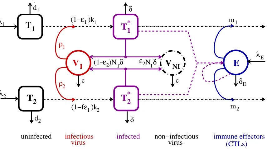
and notation is provided in Table 3.1.
m2 m1 λΕ
V
NI λ1T
1 d1 λ2T
2 d2 ρ2 ρ1T
*1T
*2(1−ε2)N
Tδ
δE
E
V
I ε2NTδ0 0 1 1 0 0 1 1
(1− )kε1
1
ε
(1−f )k
1 2 immune effectors (CTLs) uninfected δ δ infectious
virus infected non−infectiousvirus
c c
Figure 3.1: Schematic of compartmental HIV infection dynamics model. Only key pathways are indicated in the schematic – for further details, see the system of dif-ferential equations (3.1) below.
Table 3.1: State variables used in HIV model
variable description units
T1 uninfected type 1 target cells (e.g. CD4+ T-cells) cells / µl T2 uninfected type 2 target cells (e.g. macrophages) cells / µl T∗
1 infected type 1 cells cells / µl
T∗
2 infected type 2 cells cells / µl
VI infectious free virus RNA copies / ml
VN I non-infectious free virus RNA copies / ml
E cytotoxic T-lymphocytes cells / µl
The corresponding system of differential equations is principally based on the
dy-namics as suggested by Bonhoeffer, et. al. [49]. This compartment, denoted by E,
represents CTLs which lyse and thus kill infected cells. The adapted system of ODEs
is given by
˙
T1 =λ1−d1T1−(1−¯ǫ1(t))k1VIT1 (3.1a)
˙
T2 =λ2−d2T2−(1−f¯ǫ1(t))k2VIT2 (3.1b)
˙
T∗
1 = (1−¯ǫ1(t))k1VIT1−δT1∗−m1ET1∗ (3.1c)
˙
T∗
2 = (1−f¯ǫ1(t))k2VIT2 −δT2∗−m2ET2∗ (3.1d)
˙
VI = (1−¯ǫ2(t))103NTδ(T
∗
1 +T
∗
2)−cVI (3.1e)
−(1−¯ǫ1(t))ρ1103k1T1VI−(1−f¯ǫ1(t))ρ2103k2T2VI
˙
VN I = ¯ǫ2(t)103NTδ(T1∗+T
∗
2)−cVN I (3.1f)
˙
E =λE+
bE(T1∗+T
∗
2)
(T∗
1 +T
∗
2) +Kb
E− dE(T
∗
1 +T
∗
2)
(T∗
1 +T
∗
2) +Kd
E−δEE, (3.1g)
together with an initial condition vector
[T1(0), T
∗
1(0), T2(0), T
∗
2(0), VI(0), VN I(0), E(0)]T .
Here the factors 103 are introduced to convert between microliter and milliliter scales,
preserving the units from some of the published papers. In this dynamical system, the
treatment factors ¯ǫ1(t) = ǫ1u(t) and ¯ǫ2(t) = ǫ2u(t) represent the effective treatment
impact, consisting of efficacy factors ǫ1, ǫ2 and a time-dependent treatment function
0≤u(t)≤1 representing HAART drug level, whereu(t) = 0 is fully off andu(t) = 1,
fully on. See Figure 3.2 for a sample time-varying treatment protocol representing
structured therapy interruption. The relative effectiveness of RTIs is modeled by
combination therapy, we do not consider the possibility of monotherapy, even for a
limited period of time, though this could be implemented by considering separate
treatment functions u1(t), u2(t).
on
off
0
1
time(t)
u(t)
Figure 3.2: Sample control input (treatment protocol) u(t) representing structured treatment interruption. This is a schematic in that interruption periods need not be periodic and one might assume more smooth ramp functions for the absorption and dissipation of the drug.
As is common in models of HIV infection, infected cells T∗
i result from
encoun-ters between uninfected target cells Ti and infectious free virus VI in a well-mixed
environment. As noted above, this model involves two co-circulating populations
of target cells, perhaps representing CD4+ T-lymphocytes (T
1) and macrophages
(T2). The natural infection rate ki may differ between the two populations, which
could account for believed differences in activation rates between lymphocytes and
macrophages. The drug efficacy parameter ǫ1 represents an RTI that blocks new
in-fections and is potentially more effective in population 1 (T1, T1∗) than in population
2 (T2, T2∗), where the efficacy is f ǫ1, withf ∈[0,1]. The differences in infection rates
and treatment efficacy help create a low, but non-zero, infected cell steady state for
T∗
2, which is commensurate with the idea that macrophages may be an important
source of virus after T-cell depletion. The populations of uninfected target cells T1
For our efforts here we assume that both target cell types have the same death
rate δ, though this could be readily generalized as well. Infected cellsT∗
1, T
∗
2 may be
removed from the system via either natural death or by the action of immune effector
cells E described below.
To preserve simplicity in the model, we omit the chronically infected cell
compart-ments proposed in the original Callaway–Perelson model. The important qualitative
behaviors seem preserved in the model we propose and specifically modeling this
feature is not essential to our present work. In particular, the existence of a low
steady-state viral load equilibrium and sensitivity of the viral load equilibrium to the
drug efficacy is obtained with or without such compartments. We note that while
removing the chronically infected compartments does not affect the sensitivity to
treatment, the addition of immune response terms does, as discussed below.
Free virus particles are produced by both types of infected cells, which we assume
produce virus at the same rate (again this could be readily generalized to account
for different productivity). In the Callaway–Perelson model, virus only leaves the VI
compartment via natural death at ratec; there is no removal term in the ˙VI equation
representing loss of virus due to infection of a cell. One potential justification for
this omission is offered by Nelson and Perelson [45] (page 10) who suggest that this
term can be omitted since the termkiTiVI is small in comparison tocV in the typical
HIV-infected patient. They further assert that if Ti is approximately constant, one
can absorb the loss of virus due to infection into thecVI term, thus making it account
for all clearance processes.
While the arguments offered by Nelson and Perelson could justify the exclusion
of the virus removal term, we investigate situations where treatment is interrupted
abruptly, potentially effecting drastic changes in all of the cell populations under
the ˙VI equation to account for the removal of free virus that takes place when free
virions infect aT1orT2cell. We make the simplifying assumptionρi = 1, i.e., one free
virus particle is responsible for each new infection. This could easily be adapted for
multiple virus particles being responsible for each new infection by choosing ρi >1.
The action of a PI, which causes infected cells to produce non-infectious virus
VN I is modeled by ¯ǫ2. Tracking non-infectious virus is important since the
clinically-measured viral load data for patients includes total free virus (infectiousVI and
non-infectiousVN I). Model fits to data are therefore to the sumVI+VN I. However, see the
discussion below regarding the decoupling of this compartment from the remainder
of the ODE system.
Finally, the immune effectors E (CTLs), are produced in response to the
pres-ence of infected cells and existing immune effectors. The immune response assumed
here is similar to that suggested by Bonhoeffer, et al., in their 2000 paper [49], with
a Michaelis-Menten type saturation nonlinearity. The infected cell-dependent death
term in the immune response represents immune system impairment “at high virus
load”. In [49] the authors demonstrate that a model with this immune reponse
struc-ture and a latently infected cell compartment can exhibit transfer between “healthy”
and “unhealthy” stable steady states via STI, making it a good candidate for our
in-vestigation. (Indeed the same is true for the model (3.1) considered here.) We add a
source term λE to create a non-zero off-treatment steady state for E, rather than
ex-plicitly modeling immune memory. While immune effectors are not inherently present
in the absence of pathogen, they persist at low levels during infection. We note that
other immune responses models, such as those considered by Wodarz-Nowak [54] or
Nowak-Bangham [43] could be substituted if desired. However, the latter does not
appear to admit multiple stable off-treatment steady states.
lysing infected cells, causing them to explode. Thus they remove infected cells from
the system in the equations for ˙T∗
1 and ˙T
∗
2, at rates m1 and m2, respectively. Unlike
interferons, they do not directly target free virus, so there is no interaction term
with the virus compartment. As with any immune system responders, we suspect
that CTL sometimes mistarget or misidentify receptors and thus kill healthy cells or
misidentify self versus antigen, but for simplicity, we do not model that here.
While the model (3.1) explicitly includes a VN I compartment
˙
VN I = ¯ǫ2(t)103NTδ(T
∗
1 +T
∗
2)−cVN I,
it serves only as a collection compartment and does not couple with any of the other
model dynamics. Explicitly including this compartment and its dynamics
compli-cates the linear analysis of the ODE system’s stability since it introduces a zero
eigenvalue. It can be explicitly solved using variation of parameters to obtain the
necessary quantity VN I to use in model fitting as follows.
Defining G(t) = ¯ǫ2103NTδ(T1∗(t) +T
∗
2(t)) (so G(t) depends on the solution to the
remainder of the ODE system (3.1)), the solution to (3.1f) is given by
VN I(t) =VN I(0)e−ct+ Z t
0
e−c(t−s)G(s)ds. (3.2)
Given a solution to the remaining equations in the ODE system, one can compute
VN I(t) for purposes of model fitting to the clinically observed quantityV =VI+VN I.
For analysis, we therefore consider the VN I compartment as dependent on the other
dynamics.
to the ODE system (3.1):
¯
x(t) =
·
T1(t) T1∗(t) T2(t) T2∗(t) VI(t) VN I(t) E(t) ¸T
, (3.3)
where components 1–4 of ¯x are on a cells/µl scale, 5 and 6 (corresponding toVI and VN I) on a copies/ml scale, and 7 on a cells/µl scale. The differential equation model
(3.1) can therefore be summarized by
dx¯
d t = ¯g(t,x¯;q),
with q denoting model dynamic parameters and ¯g the vector of derivatives. Model
fits will be to the base-10 logarithm of these quantities (x= log10x¯) and in general, as
explained in the notation section, variables with an overbar will denote an unscaled
quantity and those without, log10-transformed variables.
3.2.1
Sample model parameters, steady states, and
treat-ment efficacy
The model (3.1) contains numerous parameters that must be assigned values before
simulations can be carried out. In specifying model parameters, to the greatest extent
possible we employ values similar to those reported or justified in the literature.
The parameters indicated in Table 3.2 are principally extracted from the Callaway–
Perelson [17] and Bonhoeffer, et al., [49] papers.
Callaway and Perelson point out that several model parameters are not available
from human or animal data. They choose the parametersλ1, k1, λ2, and k2 such that
several conditions on target cell and viral load equilibria are satisfied for their model.
Table 3.2: Parameters used in model (3.1). Those in the top section of the table are taken directly from Callaway and Perelson [17]. Parameters in the bottom section of the table are taken from Bonhoeffer, et. al. [49], with slight adjustments. The superscripts ∗
denote parameters the authors indicated were estimated from human data and ∗∗
denote those estimated from macaque data.
parameter value units description
λ1 10 ulcells·day target cell type 1 production (source) rate
d1 0.01∗∗ day1 target cell type 1 death rate
ǫ1 ∈[0,1] – RTI treatment efficacy
k1 8.0×10⁻⁷ virionsml·day population 1 infection rate
λ2 0.03198 ulcells·day target cell type 2 production (source) rate
d2 0.01∗∗ day1 target cell type 2 death rate
f 0.34 (∈[0,1]) – treatment efficacy reduction in population 2
k2 1×10⁻⁴ virionsml·day population 2 infection rate
δ 0.7∗ 1
day infected cell death rate
m1 0.01 cellsul·day immune-induced clearance rate for pop. 1 m2 0.01 cellsul·day immune-induced clearance rate for pop. 2
ǫ2 ∈[0,1] – PI treatment efficacy
NT 100∗ virions
cell virions produced per infected cell
c 13∗ 1
day virus natural death rate
ρ1 1 virionscell average number virions infecting a type 1 cell ρ2 1 virionscell average number virions infecting a type 2 cell
λE 0.001 ulcells·day immune effector production (source) rate
bE 0.3 day1 maximum birth rate for immune effectors
Kb 0.1 cellsul saturation constant for immune effector birth
dE 0.25 day1 maximum death rate for immune effectors
Kd 0.5 cellsul saturation constant for immune effector death
δE 0.1∗ day1 natural death rate for immune effectors
compartment and an added immune response. However, the conditions are closely
approximated by the model’s behavior (partially due to multiple stable equilibria) and
we believe the parameters could be adjusted to obtain the same qualitative behavior.
In general, immune response parameters are not well-known and are thus
fre-quently chosen to demonstrate model behavior in simulations. The parameters m1
and m2 represent cytopathicity of the immune effectors. Their common value m =
suggested originally by Nowak and Bangham [43]. The parameters in the ˙E equation
(3.1g) are also slightly adjusted from published values to demonstrate the possibility
of multiple stable equilibria for the model.
In order to understand the possible behaviors of the model under treatment
in-terruptions, we examine the possible equilibria to which the model dynamics might
converge. These do not depend on the dynamics for the non-infectious virus, so we
define the reduced vector xR = [¯x1, . . . ,x¯5,x¯7]T and gR(t, xR;q), the corresponding
model dynamics (derivatives). Model steady states (equilibria) result from solving
the system of six algebraic equations gR(t, xR;q) = 0 for the steady state values ˜xR,
i.e., ˜xRare the state values where derivatives are all zero. By setting ˙VN I = 0 in (3.1f)
and substituting values ofT∗
1, T
∗
2, and VIfrom ˜xR, the correspondingVN I equilibrium
follows.
To assess the stability of the equilibria, calculated steady state values ˜xR may
then be substituted for xR in the Jacobian matrix
J(xR;q) =
∂ gR(t, xR;q) ∂ xR
=
−d1−¯k1VI 0 0 0 −¯k1T1 0
0 −d2−k¯2VI 0 0 −¯k2T2 0
¯
k1VI 0 −δ−m1E 0 k¯1T1 −m1T1∗
0 k¯2VI 0 −δ−m2E k¯2T2 −m2T2∗
−k¯1103VI −¯k2103VI (1−ǫ¯2)103NTδ (1−ǫ¯2)103NTδ J5,5 0
0 0 J6,3 J6,4 0 J6,6


![Table 3.2: Parameters used in model (3.1). Those in the top section of the table aretaken directly from Callaway and Perelson [17]](https://thumb-us.123doks.com/thumbv2/123dok_us/1604676.1198431/46.612.109.539.188.525/table-parameters-model-section-aretaken-directly-callaway-perelson.webp)