R E S E A R C H
Open Access
CDSWS: coverage-guaranteed distributed sleep/
wake scheduling for wireless sensor networks
Guofang Nan
1*, Guanxiong Shi
1, Zhifei Mao
1and Minqiang Li
2Abstract
Minimizing the energy consumption of battery-powered sensors is an essential consideration in sensor network applications, and sleep/wake scheduling mechanism has been proved to an efficient approach to handling this issue. In this article, a coverage-guaranteed distributed sleep/wake scheduling scheme is presented with the purpose of prolonging network lifetime while guaranteeing network coverage. Our scheme divides sensor nodes into clusters based on sensing coverage metrics and allows more than one node in each cluster to keep active simultaneously via a dynamic node selection mechanism. Further, a dynamic refusal scheme is presented to overcome the deadlock problem during cluster merging process, which has not been specially investigated before. The simulation results illustrate that CDSWS outperforms some other existed algorithms in terms of coverage guarantee, algorithm efficiency and energy conservation.
1 Introduction
With the advances in digital signal processing, RF tech-niques and low-power hardware manufacturing and integration, wireless sensor networks (WSNs) have attracted increasing interests in recent years [1]. A WSN is structured with a certain number of tiny sensor devices, and each device has the abilities of computa-tion, storage, and communicacomputa-tion, which enable it to collect sensing data and conduct data processing tasks about the environment, and to generate and deliver helpful information on the monitored objects to the base station for decision making [2]. The appearance of WSNs has significantly changed various kinds of remote sensing applications such as environmental and ecologi-cal monitoring of natural habitats, smart homes, and military areas [3].
In order to provide high-quality data service, a multi-level of sensing coverage and network connectivity is needed in the practical implementation of a WSN. That is, any point in the region should be covered by more than one sensor. Therefore, wireless sensors are usually densely deployed on the target field [4], that is, many sensors can detect an event, deliver and receive the sensed data packets simultaneously, which will cause redundant communication overhead and thereby leads
to large amount of energy consumption. Due to the facts that wireless sensors are physically small and must use extremely limited power or energy, the network life-time is an essential consideration in sensor network applications. Moreover, a WSN is usually deployed in hostile fields or under harsh environments [5] where manually recharging batteries for sensors is not feasible, one typical alternative approach to energy saving is to turn off some sensors and activate only a necessary set of sensors while providing a good sensing coverage and network connectivity simultaneously [6]. A good sleep/ wake scheduling has to provide an even distribution of energy consumption among sensor nodes so that the network lifetime is extended [7].
Several schemes have been proposed in the literature to determine how many and which nodes should be allowed to sleep [7], and they can be divided into distributed sleep/wake scheduling schemes [8-11] and centralized sleep/wake scheduling mechanisms [12-16]. Generally, centralized sleep/wake scheduling algorithms are appro-priate only for stationary targets or moving targets with known and static movement patterns [17], and it is easy to achieve more precise scheduling results. However, for an unknown and dynamically changing movement envir-onment, the centralized sleep/wake scheduling algo-rithms are not flexible enough to adapt themselves to these changes. Another drawback for the centralized ones is that sleeping nodes should have the ability to * Correspondence: [email protected]
1Institute of Systems Engineering, Tianjin University, Tianjin 300072, China Full list of author information is available at the end of the article
receive messages all the time, and their receiving antenna cannot be switched off. In addition, a powerful base sta-tion [14] is used for centralized scheduling to perform a large amount of computation and communication tasks, and it is dificult for the base station to maintain the glo-bal information of the whole network, which will lead to a large amount of data transmission, and thereby cause more energy consumption. On the other hand, most of these distributed sleep/wake scheduling schemes make the sensors self-organized to carry out network tasks, which have less messaging cost and better adaptability to dynamic conditions [16]. Moreover, distributed algo-rithms are scalable and can work independently for a long time.
However, there are still several major limitations in prior distributed sleep/wake scheduling algorithms. First, it is inconvenient for sensors to maintain sensing cover-age and connectivity of the entire network by using these distributed algorithms due to the fact that only local information is used for sensors to decide their status. For example, in [8], an adaptive partitioning scheme called connectivity-based partition approach (CPA) was pre-sented for sleep scheduling and topology control in WSNs, CPA divides the network into several groups, only one node in each group will be selected to be active to form a backbone network. Since the communication radius of sensors is applied in group partitioning stage, the proposed algorithm ensures the effective connectivity of the network, but does not consider the problem of sensing coverage. A geographical adaptive fidelity (GAF) algorithm [18] partitions the nodes into multiple equal-size squared cells based on their geographic locations, and one node in each cell remains active, GAF also ensures network connectivity, but ignores sensing cover-age. The authors in [6] also developed a distributed adap-tive sleep scheduling algorithm (DASSA) for WSNs with partial coverage, which suits only for temperature or humidity monitoring. Second, most of the distributed algorithms [6,8,14,17,19,20] assume that only one node in each cluster or group is active while others are shut off, which is usually effective in early stage of the network lifetime, and once some nodes are failed to sense and communicate, this mechanism may lead to poor quality of service (QoS) of the network. Third, the deadlock pro-blem arising from resource contention has received little attention in the past, which will result in degraded net-work performance in distributed sleep/wake scheduling. A deadlock is a persistent and circular-wait condition in forming a cluster or a group [8], where each potential cluster head delivers a merging request message to another cluster, and may involve in a deadlock waiting indefinitely for the merging respond from other nodes while not answering other merging requests [21].
Motivated by above limitations, a novel distributed coverage-guaranteed sleep/wake scheduling algorithm called CDSWS is proposed in this article. In CDSWS, a cluster hierarchy based network framework is consid-ered, and a minimum number of nodes are selected to be active to monitor the area while maintaining better coverage and connectivity in this article. We assume in this article that communication radius of a sensor is equal to or greater than twice of its sensing radius, which has been proved that the coverage of a region implies connectivity of the network [22]. Moreover, a sensor is selected to be in sleep mode based on its sen-sing radius. That is, if a sensor is in the sleep mode, its whole working area can also be covered by other active nodes, which does not affect whole coverage perfor-mance. Thus, any point in the region can be covered by those active nodes and any two active nodes are con-nected. In addition, a dynamic node selection mechan-ism is also adopted in each cluster to maintain network performance. Unlike prior work, more sensors in each cluster are allowed to be active simultaneously. Finally, in order to overcome the deadlock problem in clusters merging, a set of rules are illustrated to avoid existing deadlocks. For each clusterhead, when it sends request to other clusters while receiving other requests simulta-neously, obtaining respond from its requesting object or answering other requests is determined by these rules, consequently, merging delay and energy consumption are reduced.
The rest of this article is organized as follows. Section 2 gives a brief literature overview. We introduce the motivation and present our solution in Section 3. In Section 4, we propose our coverage-guaranteed schedul-ing framework and the correspondschedul-ing algorithms to support our scheduling framework. In Section 5, we pre-sent simulation and experiment results to demonstrate the efficiency of the work and compare it with other scheduling techniques. Finally, the advantages and disad-vantages of the proposed scheme are discussed in Sec-tion 6.
2 Literature review
Turning off some nodes in the network and using only a necessary set of nodes for information collection and packet delivery is one popular way of energy conservation [16]. GAF uses geographic location information to divide a sensing region into equal-sized grid cells, and each cell of the grid is square shaped, only one node is active in each grid, then forms a backbone network to maintain connectivity [21]. In [24], a few nodes are selected as coordinators which remain active for packet routing, and other nodes go into the sleep state according to a sleep/ wake cycle specified by the coordinators. In [25], a node decides to go into sleep mode if there is an active neigh-bor within its sensing range, and its sleeping period is self-adjusted dynamically. Otherwise, it remains active. However, this method does not need the location infor-mation. The mechanism that randomly selected idle sen-sors to go into the sleep mode is allowed in the scheduling [26] to save energy. The data packets for sleeping nodes are temporarily stored at the active nodes in their neighbors, and the sleeping sensors wake up peri-odically to retrieve the stored packets from their neigh-boring nodes. This method usually leads to packet delay. An adaptive partitioning scheme of sensor networks for node scheduling and topology control was presented in [8] to reduce energy consumption. Sensors are parti-tioned into several groups according to the measured connectivity between pair-wise nodes, which varies prior partitioning approaches based on sensor locations. In each group, only one node is active while others are put into sleep mode. The authors formulated a constrained optimal graph partition problem to study sleep/wake scheduling with topology control. A distributed heuristic approach called CPA was proposed. The authors in [6] also developed a DASSA for WSNs with partial coverage, which does not require location information of sensors while maintaining network connectivity and satisfying a user defined coverage requirement. A common character among above scheduling schemes is that these active nodes form a backbone network to assure network con-nectivity without considering sensing coverage.
Some coverage-preserving scheduling algorithms were discussed in [17,27-29]. In [27], each node in the network autonomously and periodically makes decisions on whether to turn on or turn off itself only depending on its local neighbor information. To preserve sensing coverage, a node will turn it off when other active neighbors can help it to cover its whole working area. Optimal Coverage-Preserving Scheme (OCoPS) [28] extends the center angles calculation method described by [27], based on the proposal of a wake-up strategy, a new decision algorithm is illustrated to decide the node status by exchanging local information. Aiming at dynamic point coverage, a schedul-ing algorithm based on learnschedul-ing automata is proposed in [17], the advantage is that less auxiliary messages are
needed to be delivered between nodes, and each node in the network is equipped with a set of learning automata which determine when and which node should be in active or asleep state according to environmental information. Experimental results show that the proposed scheme out-performs the existing methods. A coverage-adaptive ran-dom sensor scheduling [29] was also presented to meet the desired sensing coverage specified by the users. How-ever, the above methods pay little attention to network connectivity.
The Sense-Sleep Tree (SS-Tree) [10] uses flow models and mathematical programming to the network in accor-dance with the classification tree structure to solve sleep scheduling. It uses the tree structure of the network sche-duling and graph theory was applied to form SS-Tree, the method has a high computing complexity and cannot work in the complex situation. The authors in [12] inves-tigated the cross-layer sleep/wake scheduling design in service-oriented WSNs, the purpose of this study is to minimize the energy consumption and guarantee that enough sensors are active to provide all required network performances. The sleep scheduling is considered to be NP-hard, and a heuristic linear programming based solu-tion is also presented. However, they assume that each service has a known requirement on the number of active sensors based on the historical service composition requests in the system, which may not be the case in practice.
More accurate scheduling results will be achieved by suing the centralized approaches, which also lead to a large amount of data transmission and computation.
Another fundamental issue is the deadlock problem in distributed computing and several deadlock avoiding mechanisms for sensor network applications have been illustrated in the prior literature. However, the afore-mentioned mechanisms were designed for distributed edge-coloring [31], determining d-dominating sets for coverage tier [32] and secure data aggregation [33]. One possible deadlock scenario will occur for sensors to self-organize into clusters or groups. However, little atten-tion has been given to the deadlock problem in sleep/ wake scheduling.
3 Motivation and major considerations
In this section, we analyze several limitations of the existing studies that motivate us to make the nodes self-organize into clusters in pure distributed manner. We also give the main strategies to overcome these limitations.
3.1 Motivation
In CPA, sensors are partitioned into several groups based on their measured connectivity between nodes instead of their location information. The process of CPA starts from the initial partition where each node forms a unique group, and two groups are continuously merged into a larger one. CPA has more flexibility because it can achievek-connectivity of the backbone network and switch node status within each group after the partitioning process is finished. Meanwhile, con-strained optimal graph partition problem is used to
for-mulate group partitioning, and a distributed
implementation of CPA is illustrated. However, it still suffers from several limitations.
First, sensing coverage and network connectivity are two important issues that considerably influence the QoS of an entire network system. However, CPA was designed with the purpose of maintaining the network connectivity, and the sensing coverage was not taken into consideration. The lack of coverage guarantee will clearly render the network more prone to node failures and produce more coverage holes, which will lead to poor network monitoring performance.
Second, in the group merging process of CPA, a prior-ity value is assigned for each two completely adjacent groups, which is given by priority=k1(1-a) +k2b+R,
wherek1 andk2are coefficients,a indicates the level of
equivalence between these two groups,b is the ratio of energy in these two groups to the total energy of the entire network,Ris a random value uniformly distribu-ted in [0,1]. As a result, the appropriate assignment enables pairwise groups with a lower priority value to
merge first. It is noteworthy that the calculation of the total energy has to rely on a centralized scheme of infor-mation collection that is apparently run contrary to the concept of distributed computation. In practice, numer-ous data relays among nodes are required to figure out the total energy of the network, thereby increasing the execution complexity. Apart from the execution com-plexity, the data arrived at sensor nodes tend to be out-of-date due to the severe network delay, so the priority value that obtained may be imprecise.
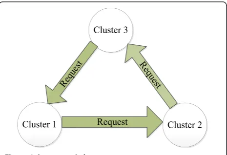
Third, severe deadlocks potentially exist during the process of group merging in CPA. For instance, a request circle will occur among three groups when each group sends simultaneously a merging request to its next group in the circle as shown in Figure 1, and each group do not answer the merging request from its last group. Thus, a deadlock is generated and no further merging process will continue. Generally, a time-out mechanism or a multi-round technique can be exploited to address deadlock problems. However, these approaches will incur undesirable resources abuse in terms of time delay and energy consumption.
Finally, in the startup phase of nodes scheduling in CPA, a large communication over-head will be produced because each node in one group broadcasts a message to announce its inclination to be the head node, which will results in not only energy inefficiency but transmis-sion interferences among sensor nodes. Besides, the node with the maximum residual energy will be selected as the head theoretically by setting the time delay for each node inversely proportional to its residual energy. However, it is usually not the case in practice because of the network delay and poor signal quality.
In our scheme, we modify the group merging con-straints and priority formulation, and then introduce a dynamic unlocking method in conjunction with a novel nodes scheduling scheme. In consequence, substantial
Cluster 1 Cluster 2
Cluster 3
Request
Request
Request
improvement will be achieved in terms of coverage sup-port and algorithm efficiency.
3.2 Sensing coverage guarantee
Our CDSWS partition sensors into several clusters based on their sensing coverage rather than measured connectivity. Since it has been proven that if the radio range of the sensor is equal to or greater than twice the sensing range, i.e.,rc ≥ 2rs, complete sensing coverage
implies network connectivity [22]. In other words, in case ofrc ≥ 2rs, we only need to consider the sensing
coverage.
Consider that the sensor nodes are divided into multi-ple clusters. At any given time, only a few sensors are selected from different clusters to be in active status, while others are put into sleep mode to conserve the precious energy. To maintain a nearly full coverage, the area that can be monitored by the active sensors should be almost equal to the area that can be monitored by all sensors. Hence, the coverage disks of these active sen-sors should intersect one another within each cluster. However, if two neighboring clusters are not densely connected, they cannot be merged into a larger one.
In terms of minimizing the number of sensors used in deployment, an efficient method to cover the monitored region is to deploy sensors in a triangular pattern with
√
3rsas the length of a side [34], that is, if the distance
between each two nodes within the same cluster is no more than√3rs, their coverage disks will be densely
connected.
In CDSWS, the concept of neighboring clusters is defined as follows:
Definition 1 (Neighboring clusters): Let Aand Bbe two different clusters, for any node xi in A and any
nodexjinB,AandBare said to be neighboring clusters
if
d(xi,xj)≤
√
3rs (1)
where,d(xi,xj) denotes the distance betweenxiandxj.
Denote that the numbers of sensors in A and Bare
NA and NB. For any xi Î A and xj Î B, if
d(xi,xj)≤
√
3rs, then the connection value between xi
andxjis referred to be 1, say cij= 1. Thereby, the
con-nectivity intensity between clustersAandBcan be cal-culated as
CAB= NA
i=1 NB
j=1 cij
NA×NB (2)
The calculation of connectivity intensity is executed along with the cluster-forming operation. Clusters A andB can be merged only whenCAB= 1, i.e., AandB
are neighboring clusters. Moreover, in order to
guarantee the coverage-connectivity in the scheduling process, there must exist at least one other cluster (denoted as D) that can satisfyCADand CBD
simulta-neously. Hence, the connectivity of the area covered by active sensors of these given two clusters Aand Bcan be guaranteed.
3.3 Priority design in cluster merging
In cluster merging, each two adjacent clusters that matches sensing coverage requirement is assigned with a utility value. For a given cluster, there may exist several candidate clusters that can be merged with, and only one cluster is allowed to be merged with the given cluster in our algorithm. Therefore, we rank the candidate merging clusters according to their utility value and the one with lower utility value is merged ultimately until no candidate merging clusters satisfy merging requirement.
For a given cluster, several candidate clusters may exist to form different pairwise clusters, if two or more of them have not only the same but the least cluster size. The problem that which one should be merged with the given cluster will become a challenge for the distribute environment. In our algorithm, we introduce a random value distributed in 0[1] in the priority formu-lation to solve this issue. Specifically, to balance energy distribution among all clusters, merging priority should be given to the cluster pairwise with the least sensors. One reason is that it will spend more time for sensor nodes in small-size clusters to be in active status due to periodically alternative working mechanism, which thereby leads to unbalanced energy distribution among clusters. Furthermore, it is convenient for the cluster heads to maintain only the sensor number information of their clusters, thus avoiding collection of the nodes’ residual energy which is hard to implement. For any two adjacent clustersAiandAj, the number of sensors
in them are size(Ai ) and size(Aj ), respectively. The
priority value is given by
priority = size(Ai) + size(Aj) +R (3)
where,R is a random value uniformly distributed in [0,1].
3.4 Dynamic refusal scheme
A purely distributed algorithm is characterized by con-currency which may bring deadlocks. There are four necessary and sufficient conditions for a deadlock to occur.
(b) Hold and wait condition. Processes already holding resources may request new resources held by other pro-cesses. During cluster merging, each cluster holds a resource (i.e., the cluster itself) and meantime waits for another cluster that holds the same resource to merge with.
(c) No preemption condition. No resources can be forcibly removed from a process that holds it, and resources can be released only by the explicit action of the process. A cluster who broadcasts a merging request would not accept a merging request from other clusters.
(d) Circular wait condition. Two or more processes form a circular chain where each process waits for a resource that the next process in the chain holds. Given that the sensor nodes are homogeneous and the clusters are equal with each other, it is reasonable to suppose that circular waiting does exist during cluster merging.
Considering the severe consequence brought by dead-lock, it is necessary to design an approach to break at least one of the four conditions that would produce a deadlock. Here, we introduce a dynamic refusal scheme to combat the deadlock problem through avoiding cir-cular-waiting.
Specifically, each initiative cluster opens a timer and creates a variable named WaitPossibility after delivering the request for merging, the value of which indicates the possibility of accepting the request and refusing other requests. This value is initially set to 0.9, and then decreases by a fixed rate with time until it reaches zero. During cluster forming process, a cluster that receives a merging request will first check the source of the request rather than directly accept it, if the source is one of its merging targets, the cluster can deliver an acknowledge to accept the request with a possibility of the value of WaitPossibility (particularly, 0 means a refusal).
3.5 Sleep/wake scheduling
Due to the fact that sensors within the same cluster are densely deployed, the connectivity of the area covered by active sensors can be guaranteed. It is noteworthy that the selection of active sensors in different clusters is independent from others. Thus, to evaluate the con-nectivity between the cluster and its neighboring clus-ters, a connection value for each cluster (denoted as A) is calculated as follow.
CONA=
B∈neighbor(A)
CAB (4)
It can be seen from (4) that the connection value for each cluster is evaluated by the summation of the con-nectivity intensities betweenAand its neighboring clus-ters. In addition, we can see that ifCONA is larger than
a given threshold h, only one sensor with the highest energy is needed to be active. Otherwise, two sensors are required to keep in active mode in clusterA.
4 CDSWS: coverage-guaranteed distributed sleep/ wake scheduling
We considered the scenario where nodes are densely deployed into a region of interest. That means that only some nodes are selected to be active to maintain sensing coverage and network connectivity. The goal of our CDSWS is to partition these nodes into clusters, and at least one node in each cluster is allowed to be active to perform monitoring task. Meanwhile, nodes in the same clusters work alternatively to save energy. Our CDSWS has three major phases: initialization phase, cluster forming phase and sleep/wake scheduling phase.
In this scheme, each cluster is a basic running unit. First it runs an initiative thread to search any clusters that can be merged with, and then opens a listener for receiving messages from other clusters. The initiative thread can be divided into two parts, i.e., initiative searching and merging. In order to control the distribu-ted process, we specify six states for each cluster to dif-ferentiate its working status.
Decision
A cluster is said to be in Decision state when it has not sent its merging request or has already finished a round of merging process, and this cluster can accept merging requests from other clusters in this state.
Contending
A cluster that has decided its merging target and has sent the request message will go into this state so that this cluster can deal with the request from other clusters through the dynamic refusal mechanism.
Waiting
A cluster will be switched into Waiting state immedi-ately after responding an initiative cluster, and wait for a corresponding merging instruction until waiting delay exhausts or receiving a instruction.
Locking
The cluster will stop searching, namely entering Locking state, while all of its neighboring clusters enter the mer-ging process. Its locking level is determined by the num-ber of lock messages from its neighboring clusters.
Merging
Disposed
When two clusters are successfully merged into a new and larger one, their IDs will be disposed from the memory of their respective head nodes and neighbors.
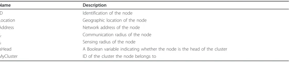
Each cluster switches between these six states in the cluster forming process until the whole process ends. Besides, because the process runs in a distributed man-ner, it is necessary for the nodes and cluster heads to memorize several important variables of the algorithm, which are shown in Tables 1 and 2.
4.1 Initialization phase
In the initialization phase, sensor nodes transmit and receive packets randomly after they are deployed. There-fore, every node obtains the location information of its neighbors. The proposed algorithm is a distributed heuristic algorithm, it starts from the initial partition where each node forms a unique cluster while being the head itself and opens a listener preparing to receive messages from other clusters. These clusters enter Lock-ing state first, and then broadcast a message to search for neighbors and memorize their IDs while wait responses. Afterwards, the cluster head sends an UPDATE message to its neighbors, which contains the basic information of the cluster. As long as a cluster receives an UPDATE message from each of its neigh-bors, it goes into Decision state. At the end of the initia-lization phase, nodes move to the cluster forming phase where two potential clusters will be merged into a large one through a user predefined iterative process until no cluster pairs can be further merged.
4.2 Cluster forming phase
Once all the clusters have entered Decision state, each of them creates a thread to run the initiative searching pro-cess. Meanwhile, its listener keeps open and waits for messages. The initiative searching process consists of three steps. First, each cluster calculates its merging priority by using the information of its neighbors as men-tioned in Section 3. If a cluster finds a target to merge with, it will memorize the ID of the target and enter into Contending state and it will stop the whole merging pro-cess. Second, under the former circumstance in step 1,
the cluster delivers a MERGE_REQ message to the target and opens a timer while the value of WaitPossibility is set to 0.9 which will be decreased over time. Third, the cluster waits for a reply from the target until its state is turned into Disposed. The procedure of initiative search-ing is summarized in Algorithm 1.
The listener of a cluster works all the time during the whole merging process, and it responses each received message from other clusters. To distinguish the received messages with distinct functions, we design a number of message heads for the listener and their corresponding trigger shown in Algorithms 2, 3, 4, 5 and 6.
MERGE_REQ
It is a merging request which is sent by an initiative cluster to its merging target.
MERGE_ACK
It is an acknowledgement of MERGE_REQ. A cluster that receives a MERGE_REQ and in Contending or Waiting state will first check the source (namely ID of this source node) of the message according to the content of its Mer-gingTarget. If the source is one of its merging target, the cluster either deliver a MERGE_ACK to accept the request or refuse it by using the dynamic refusal scheme. MERGE_NAK
It is a refusal of MERGE_REQ. A cluster that receives a merging request but not in Decision or Contending state will deliver a MERGE_NAK to refuse this request. As to a cluster that receives a MERGE_NAK, its state will transfer into Decision and then initiate next searching.
Table 1 Variables in node
Name Description
ID Identification of the node
Location Geographic location of the node
Address Network address of the node
rc Communication radius of the node
rs Sensing radius of the node
IsHead A Boolean variable indicating whether the node is the head of the cluster MyCluster ID of the cluster the node belongs to
Table 2 Variables in cluster head
Name Description
ID Identification of the cluster Head Head of this cluster Members Members in the cluster Neighbors Neighbors of this cluster State Current state of the cluster
WaitPossibility Possibility of this cluster refusing requests from other clusters
MERGE
This is a merging rule for two clusters. If a cluster is not in MERGING state, it will check whether the merging message is from its mergingTarget. If yes, the merging begins and both of these clusters first turn their states into Merging, the cluster with more sensor nodes will be the initiative one and its cluster head will record the information of the new merged cluster. After two clus-ters are merged, they will be in DECISION state. CANCEL
It is a cancellation of its former merging request sent by an initiative cluster to its merging target. A cluster in the state of Waiting will reset the content of Merging-Target and go into Decision state when it receives this CANCEL message.
LOCK
It is a locking signal. Clusters stepping into Merging state, namely starting merging, will broadcast a LOCK message. A cluster that not being in the state of Mer-ging or Waiting will raise its locking level by 1 while receiving one LOCK, and go into the state of Locking while the locking level is high than 0.
UPDATE
It carries information of an initiative cluster that has already been merged with another one. When a cluster in the state of Locking receives a UPDATE message, its locking level will decrease by 1, and it will transfer into Decision state if the lock level is 0.
DISPOSED
Its content is the information of a passive cluster that has been merged by another. When the cluster in the state of Locking receives this message, its lock level will decrease by 1 as well as receiving a UPDATE message.
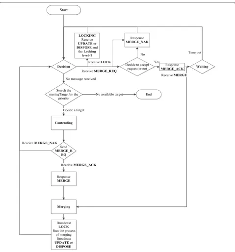
The whole flow diagram of cluster forming is shown in Figure 2.
4.3 Sleep/wake scheduling phase
Once the cluster forming process is completed, every cluster starts the process of sleep/wake scheduling. In order to save energy, only one or two nodes with high-est residual energy in each cluster are required to keep active, while others turn off their radio devices, i.e., being asleep.
In the continuous data-gathering mechanism, each sen-sor node in a given cluster works periodically. At the beginning of sleep/wake scheduling, all the nodes have to keep active to configure the network, i.e., active node(s) selection. Generally, node(s) with highest energy will undertake the sensing task in a cluster. The cluster head decides which node(s) should be in active state. In one cluster, the cluster head delivers a WORK message to order the selected node(s) to perform its/their duty as working node(s), moreover, one of which is told to be the
head node in the next period. Meanwhile, the head delivers a SLEEP message to all of the rest nodes. All the sleeping nodes will wake up and send a WORK_REQ to the cluster head to participate in node(s) selection when the next round comes. While receiving WORK_REQs from all the sleeping nodes in the cluster, the head will run the process of selecting active nodes. The procedures that deal with distinct messages are summarized in Algorithm 7.
4.4 Time complexity analysis
Now we analyze the complexity of CPA and CDSWS. We only analyze cluster or group merging phase because it significantly affects the time connectivity of whole algo-rithms. Assume thatnsensors are deployed into an area of interest, and the average connectivity degree ism. In CPA, the connectivity level for every node is firstly mea-sured, and complexity of calculating the connectivity level isO(n2). Another important phase is the group mer-ging which includes calculating mermer-ging priority and ranking. In the process of calculating merging priority, the maximum value of connectivity for each group ism. So the complexity of executing union or intersection operation for every two candidate groups isO(m2). It is also required to measure the level of equivalence between these two groups, which can be indicated as a cartesian product of two groups, so the connectivity becomes Om× n
m
×Om2, that isO(nm2
). Further, the ratio of energy in two groups to the total energy of the entire net-work is then calculated, and the complexity isO(n+ 2m). Thus, the complexity of calculating merging priority is approximate toO(nm2). In the process of sorting mer-ging priority for all candidate mermer-ging groups, because the number of groups is uncertain in each iteration and the maximum value isn, the complexity can be denoted asO(n). Therefore, in each iteration of the merging and ranking phase, the complexity isO(n) +O(nm2), and the maximum number of iterations does not exceed n, so the complexity is O(n2) + O(n2m2). Therefore, the whole complexity of CPA isO(n2) +O(n2m2) +O(n2) = O((m2+ 2)n2).
above theoretical analysis due to concurrency of nodes, even so, our CDSWS still performs better than CPA in time complexity.
5 Performance evaluation 5.1 System configuration
Our algorithm is simulated with homogenous sensors randomly deployed in square areas. Both the
communication radius and sensing radius are fixed in each experiment, and the value of which varies in dif-ferent experiments. It is also assumed that each node has an initial energy of 500 Units and 1 s of work costs 1 Unit of energy. To simulate the behavior of sensor nodes as in real environment, a 30 ms delay is added in each communication.
Start
Search the meringTarget by the
priority
No message received
Contending
Decide a target
Send
MERGE_R EQ
End No available target
Response
MERGE
ReceiveMERGE_ACK
Merging
Broadcast
LOCK
Run the process of merging
Broadcast
UPDATEor
DISPOSE
ReceiveMERGE_NAK Decision
LOCKING
Receive
UPDATEor
DISPOSEand
theLocking
level<1
ReceiveLOCK
Response
MERGE_ACK
Decide to accept request or not ReceiveMERGE_REQ
Yes No Response
MERGE_NAK
Waiting
ReceiveMERGE
Time out
5.2 Cluster merging
The dynamic refusal scheme is a key technique to tackle circular waiting, which further improves the efficiency of clusters forming. In this experiment, we evaluate the impact of dynamic refusal scheme on cluster forming in terms of merging time.
Here, a WSN is con figured with different sensor den-sities (say 1-5 sensors per grid) randomly deployed in a 100 × 100 square area which is divided into 25 grids with the size of 20 × 20 for each. In order to compare the performance of our algorithm with that of CPA, the communication radius and sensing radius are set equal to those in CPA, say40√5and20√5, respectively. To reduce the effects of stochastic factors involved in the test, we run this experiment 30 times and then average the results.
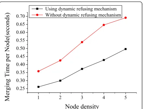
Figure 3 shows that the merging efficiency is signifi-cantly improved by using the dynamic refusal scheme, especially for the deployments with higher node density. For example, approximately 30 s is reduced with the deployment of five nodes per grid. Figure 4 shows that the merging time cost per node decreases to around 0.25 s by a 0.1 s from nearly 0.35 s with the deployment of one node in each grid, and even 0.2 s is saved when there are five nodes in each grid. With higher node den-sity, both the total merging time and the merging time per node increase almost linearly, which should be attributed to the increasing frequency of merging and information exchanges. However, both of them can be significantly reduced by using our dynamic refusal scheme, this can be interpreted under the scenario where circular waiting will more possibly occur as node density increases, the efficiency of cluster forming will deteriorate due to frequent and unavoidable failures to merging handshaking.
In addition, a comparison of average cluster size is made between CPA and our CDSWS. The table below provides the comparison result when the node density is 5. Because parameter controls the minimum degree of the 2-induced graph of the final partition in CPA [8], we list four different clustering results with different set-tings. We notice from Table 3 that the average size of each cluster of our algorithm is larger than that of CPA. This is because the merging constraint in CDSWS is relaxed while CPA does not consider the coverage guar-antee. In our CDSWS, the average size of each cluster is larger that that of CPA, which means that less clusters are produced. Moreover, in most cases, the connection value between a cluster and its neighbors is larger that the threshold, only one sensor in each cluster needs to be in active state. Therefore, a minimum number of nodes are selected to be active.
5.3 Sleep/wake scheduling
In this section, we investigate the effects of sleep/wake scheduling. The simulation region is a 100 × 100 square area which is divided into 10 × 10 grids with a grid of 10 × 10 for each. The communication radius and sen-sing radius are set to40√5and20√5, respectively, as the same in the cluster forming part. First, we compare our algorithm with CPA in terms of the number of
1 2 3 4 5 Using dynamic refusing mechanism Without dynamic refusing mechanism
Figure 3Merging time VS node density.
1 2 3 4 5
Using dynamic refusing mechanism Without dynamic refusing mechanism
Me Figure 4Merging time per node VS node density.
Table 3 Average cluster size produced by CDSWS and CPA
Partition approach Average cluster size
CDSWS 9.4
CPA (mindeg = 2) 7.0
CPA (mindeg = 3) 6.0
CPA (mindeg = 4) 5.5
working nodes in the process of sleeping scheduling. Table 4 shows that the number of working nodes in our algorithm during each working round is less than that in CPA, especially when h= 2.4, it achieves the least working nodes, i.e., only 60 nodes for node density 2 and 64 nodes for node density 3. Furthermore, Table 5 also indicates that the coverage rate reaches more than 99% with different values ofh.
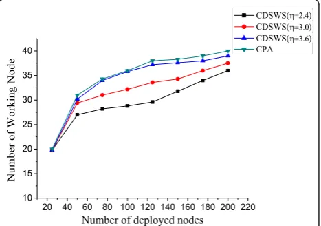
We also show the impact ofhon the number of work-ing nodes. In this example, the communication radius and sensing radius are set to 20 and 10, respectively.
Figure 5 illustrates the general trend of the number of working nodes. With the growth of the number of deployed nodes, the numbers of working nodes experi-ence a sharp increase first, followed by a comparatively steady and marginal rise. But the corresponding twists show a little difference, say around 75 for the 50 × 50 area. More importantly, the value of shows a strong cor-relation with the number of working nodes. That is, more working nodes are required to achieve a higher value of h. Moreover, because the average size of each cluster in our scheme is larger that that of CPA, the number of working nodes by our CDSWS is thereby smaller that that of CPA.
5.4 Coverage guarantee
In this section, we study the coverage issue. Here, the monitoring area is 50 × 50 which is divided into 25 grids. The communication radius and the sensing radius are 20 and 10, respectively.
In Figure 6, we observe that the coverage rate becomes higher with the increasing number of deployed sensors. We also investigate the impacthof on sensing coverage in Figure 6. Here,his a threshold that controls how many sensors are selected to be active. When deployed sensors are fixed, hlarger will lead to more active nodes, which thereby improves the whole sensing coverage. However,hhas only a small influence on the sensing coverage for the scenario where sensors are den-sely deployed. In addition, the coverage rates generated by CDSWS and CPA can achieve almost complete cov-erage when more than 150 nodes are deployed into the region.
Another experiment is carried out to capture the effect ofhon network coverage with the network running. The results are shown in the Figure 7. In the earlier stage, where the energy of each node is sufficient, the network coverage keeps steady. A higher level and a higher level of coverage is always with a higher value ofh. Then, the figure shows a slight fall in the coverage after a long steady process due to energy consumption. Finally, the network coverage degrades dramatically as the energy consumption is aggravated. In contrary to the earlier stage, a higher value ofhwill result in a lower coverage level. The reason is that more active nodes are required to maintain a higher level of network coverage (denoted by a higher value ofh), and nodes will consume energy faster until their failures. Thus, it is impossible to keep a higher level of network coverage by more active nodes. Accordingly, there is an essential tradeoff between cover-age guarantee and network lifetime, that is, a higherh indicates a better coverage but a shorter network lifetime, and vice versa. Meanwhile, we simulated the trend of the coverage performance of CPA with the network running. It also shows a slight fall and performs worse than CDSWS whenhis set to 2.4 and 3.0.
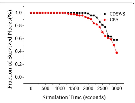
5.5 Network survivability
Finally, we evaluate our CDSWS from the perspective of network survivability which mainly involves the energy consumption of nodes during their working period.
Table 4 Number of working nodes needed by using CDSWS and CPA
Number of working nodes Destiny = 2 Destiny = 3
CDSWS (h= 2.4) 60 64
CDSWS (h= 3.0) 69 75
CDSWS (h= 3.6) 71 87
CPA (mindeg = 2) 66 70
CPA (mindeg = 3) 76 81
CPA (mindeg = 4) 88 90
Table 5 Coverage performance evaluation by our CDSWS under different value ofhand different node-density deployments
Coverage h= 2.4 (%) h= 3.0 (%) h= 3.6 (%)
Destiny = 1 99.575 99.753 99.920
mDestiny = 2 99.827 99.895 100
Destiny = 3 100 100 100
20 40 60 80 100 120 140 160 180 200 220 10
15 20 25 30 35 40
N
um
ber of W
orki
ng N
ode
Number of deployed nodes
CDSWS( )
CDSWS( )
CDSWS( )
CPA
Because energy consumption in cluster forming phase is comparatively low, it is not included in this example.
Figure 8 shows a comparison between CDSWS and CPA in terms of fraction of survival nodes. Apparently, our algorithm has a stronger survivability than CPA, especially at the end of network lifetime since the sche-duling by CDSWS makes the energy consumption of nodes in each cluster more balanced and needs fewer working nodes than CPA. In other words, nodes in net-work with CDSWS have a considerably long survival-cycle.
6 Conclusion
This article studied the sleep/wake scheduling problem in WSNs and proposed a new CDSWS to improve net-work performance. There are three advantages in this algorithm, i.e., coverage guarantee, algorithm efficiency, and energy balance. Coverage is a fundamental QoS of topology control in WSNs, we studied coverage
provision based on a prior proof that if the radio range of sensor is equal to or greater than twice the sensing range, then complete coverage implies connectivity, as a result, the network connectivity is provided as well. Sec-ond, algorithm efficiency is another essential aspect of our proposed algorithm. Due to the fact that inefficient ones always produce long time delay and energy dissipa-tion, this problem was thereby investigated by avoiding deadlock during cluster forming phase. Accordingly, we designed a dynamic refusal scheme to break circular-waiting by setting a time-varying possibility in each clus-ter, which determines whether a merging request should be accepted. The last but not least important, we obtained an energy-balanced network by allowing more than one node in each cluster to keep in an active state. Simulations were conducted to evaluate the performance of our proposed algorithm. The results illustrate that CDSWS outperforms existing algorithms with respect to coverage guarantee, algorithm efficiency and energy conservation.
Algorithm 1 - Procedure of initiative searching
1 :forsearch for themergingTargetif it exists { 2 : if the state of the cluster isDecision{ 3 : set the state of the clusterContending; 4 : if the state of the cluster is notDisposed{
5 : sendMERGE_REQtomergingTarget;
6 : }
7 : setWaitPossibility= 0.9;
8 : while the state of the cluster is notDecision{
9 : set the WaitPossibility-= 0.2 every 100
milliseconds;
10: if the state of the cluster isDisposed
11: return;
12: }
13: set delay with 1000*size(cluster) milliseconds;
14: }
Figure 6Coverage effect in area of 50 × 50.
0 500 1000 1500 2000 2500 3000
50
Figure 7Coverage with 200 nodes in area of 50 × 50.
Algorithm 2 - Trigger for MERGE_REQ
1 : caseMERGE_REQ:
2 : if the state of cluster isDecisionorContending{
3 : ifmergingTarget is null or the message is from
mergingTarget{
4 : responseMERGE_ACK;
5 : set the state of clusterWAITING;
6 : set a delay for waiting; 7 : } else {
8 : if a random number <WaitPossibility{
9 : responseMERGE_ACK;
10: } else {
11: ifmergingTargetis not null{
12: sendCANCELtomergingTarget;
13: }
14: responseMERGE_ACK;
15: set the state of clusterWAITING;
16: set a delay for waiting;
17: }
18: }
19: } else {
20: response MERGE_ACK;
21: }
Algorithm 3 - Trigger for MERGE_ACK
1 : caseMERGE_ACK:
2 : if the state of cluster isContendingorWaiting {
3 : ifmergingTarget is null or the message is from
mergingTarget{
4 : responseMerge;
5 : sendMerge to itself;
6 : }
7 : }
Algorithm 4 - Trigger for MERGE
1 : caseMERGE:
2 : if the state of the cluster is notMERGINGand the message is frommergingTarget{
3 : set the state of the clustersMERGING; 4 : broadcastLock;
5 : if the size of the cluster > the size of
merging-Target{
6 : merge themergingTarget;
7 : broadcastUPDATE;
8 : } else if the size of the cluster==the size of
mer-gingTarget{
9 : if (theIDof the cluster < theIDof merging-Target) {
10: merge themergingTarget;
11: broadcastUPDATE;
12: } else {
13: broadcastDISPOSED;}
14: merged bymergingTarget;}
15: } else {
16: broadcastDISPOSED;
17: merged bymergingTarget;
18: }
19: set the state of clustersDECISION; 20: }
Algorithm 5 - Trigger for UPDATE
1 : caseUPDATE:
2 : refresh the information of the source cluster; 3 : if the state of the cluster isLOCKING { 4 : the locking level -= 1;
5 : if the locking level == 0;
6 : set the state of the clusterDECISION; 7 : }
Algorithm 6 - Trigger for DISPOSED
1 : caseDISPOSED:
2 : delete the record of the source cluster; 3 : if the state of the cluster isLOCKING { 4 : the locking level -= 1;
5 : if the locking level == 0;
6 : set the state of the clusterDECISION;} 7 : }
Algorithm 7 - Sleep/wake Scheduling
1 : caseWORK:
2 : response SLEEP;
3 : start sensing;
4 : set the node cluster head;
5 : caseSLEEP:
6 : stop sensing;
7 : set the node normal cluster members;
8 : caseWORK_REQ:
9 : if the number of the WORK_REQ message
received{
10: select a node remains the highest energy; 11: if theCONof the cluster <h{
12: select another node remains highest energy
13: }
14: }
15: sendWORKto the nodes selected;
16: sendSLEEPto other nodes;
Acknowledgements
This research is partially supported by research grants from the National Science Foundation of China under Grant Nos. 70701025 and 71071105, the Program for New Century Excellent Talents in Universities of China under Grant No.NCET-08-0396, and a National Science Fund for Distinguished Young Scholars of China under Grant No.70925005, and the Program for Changjiang Scholars and Innovative Research Team in University.
Author details
1
Institute of Systems Engineering, Tianjin University, Tianjin 300072, China 2Department of Information Management and Management Science, Tianjin University, Tianjin 300072, China
Competing interests
The authors declare that they have no competing interests.
References
1. CK Ting, CC Liao, A memetic algorithm for extending wireless sensor network lifetime. Inf Sci.180(24), 4818–4833 (2010). doi:10.1016/j. ins.2010.08.021
2. GF Nan, MQ Li, Energy-efficient query management scheme for a wireless sensor database system. EURASIP J Wirel Commun Netw.2010, 1–18 (2010) 3. K Kalpakis, K Dasgupta, P Namjosh, Efficient algorithms for maximum
lifetime data gathering and aggregation in wireless sensor networks. Comput Netw.42(6), 697–716 (2003). doi:10.1016/S1389-1286(03)00212-3 4. H Jun, W Zhao, MH Ammar, EW Zegura, C Lee, Trading latency for energy
in densely deployed wireless ad hoc networks using message ferrying. Ad Hoc Netw.5(4), 444–461 (2007). doi:10.1016/j.adhoc.2006.02.001 5. A Chehri, P Fortier, M Tardif, UWB-based sensor networks for localization in
mining environments. Ad Hoc Netw.7(5), 987–1000 (2009). doi:10.1016/j. adhoc.2008.08.007
6. T Yardibi, E Karasan, A distributed activity scheduling algorithm for wireless sensor networks with partial coverage. Wirel Netw.16(1), 213–225 (2010). doi:10.1007/s11276-008-0125-2
7. E Bulut, I Korpeoglu, Sleep scheduling with expected common coverage in wireless sensor networks. Wirel Netw.17(1), 19–40 (2011). doi:10.1007/ s11276-010-0262-2
8. Y Ding, L Wang, L Xiao, An adaptive partitioning scheme for sleep scheduling and topology control in wireless sensor networks. IEEE Trans Parallel Distrib Syst.20(9), 1352–1365 (2009)
9. JJ Niu, Distributed self-learning scheduling approach for wireless sensor network, in2nd International Conference on Future Computer and Communication, Wuhan, China, pp. 253–257 (21–24 May 2010) 10. RW Ha, PH Ho, XS Shen, Cross-layer application-specific wireless sensor
network design with single-channel csma mac over sense-sleep trees. Comput Commun.29(17), 3425–3444 (2006). doi:10.1016/j. comcom.2006.01.019
11. B Chen, K Jamieson, H Balakrishnan, R Morris, SPAN: an energy-efficient coordination algorithm for topology maintenance in ad hoc wireless networks. Wirel Netw.8(5), 481–494 (2002). doi:10.1023/A:1016542229220 12. JP Wang, DY Li, GL Xing, HW Du, Cross-layer sleep scheduling design in
service-oriented wireless sensor networks. IEEE Trans Mobile Comput.9(11), 1622–1633 (2010)
13. NA Pantazis, DJ Vergados, DD Vergados, C Douligeris, Energy efficiency in wireless sensor networks using sleep mode TDMA scheduling. Ad Hoc Netw.7(2), 322–343 (2009). doi:10.1016/j.adhoc.2008.03.006
14. Y Wu, S Fahmy, NB Shro, Sleep/wake scheduling for multi-hop sensor networks: non-convexity and approximation algorithm. Ad Hoc Netw.8(7), 681–693 (2010). doi:10.1016/j.adhoc.2010.02.002
15. T Yardibi, E Karasan, A distributed activity scheduling algorithm for wireless sensor networks with partial coverage. Wirel Netw.16(1), 213–225 (2010). doi:10.1007/s11276-008-0125-2
16. E Bulut, I Korpeoglu, DSSP: a dynamic sleep scheduling protocol for prolonging the lifetime of wireless sensor networks, in21st International Conference on Advanced Information Networking and Applications Workshops, Niagara Falls, Canada, pp. 725–730 (21–23 May 2007)
17. M Esnaashari, MR Meybodi, A learning automata based scheduling solution to the dynamic point coverage problem in wireless sensor networks. Comput Netw.54(14), 2410–2438 (2010). doi:10.1016/j.comnet.2010.03.014 18. Y Xu, J Heidemann, D Estrin, Geography-informed energy conservation for Ad Hoc routing, inProceedings of the 7th Annual International Conference on Mobile Computing and Networking, Rome, Italy, pp. 70–84 (July 2001) 19. M Peng, Y Xiao, PP Wang, Error analysis and Kernel density approach of
scheduling sleeping nodes in cluster-based wireless sensor networks. IEEE Trans Veh Technol.58(9), 5105–5114 (2009)
20. TR Sheltami, E Shakshuki, Neighbor-aware clusterhead with different sleep scheduling protocols, inInternational Conference on Parallel Processing, Portland, USA, pp. 143–147 (8–12 Sept 2008)
21. YB Ling, SG Chen, CYJ Chiang, On optimal deadlock detection scheduling. IEEE Trans Comput.55(9), 1178–1187 (2006)
22. XR Wang, GL Xing, CY Zhang, CY Lu, R Pless, C Gill, Integrated coverage and connectivity configuration in wireless sensor networks, inProceedings of the 1st International Conference on Embedded Networked Sensor Systems, Los Angeles, USA, pp. 28–39 (2003)
23. L Wang, Y Xiao, A survey of energy-efficient scheduling mechanisms in sensor networks. Mobile Netw Appl.11(5), 723–740 (2006). doi:10.1007/ s11036-006-7798-5
24. B Chen, K Jamieson, H Balakrishnan, R Morris, Span: an energy efficient coordination algorithm for topology maintenance in Ad hoc wireless networks. Wirel Netw.8(5), 481–494 (2002). doi:10.1023/A:1016542229220 25. F Ye, G Zhong, L Lu, L Zhang, PEAS: a robust energy conserving protocol for long-lived sensor networks, in10th IEEE International Conference on Network Protocols, Los Angeles, USA, pp. 200–201 (2002)
26. W Ye, J Heidemann, D Estrin, An energy-efficient MAC protocol for wireless sensor networks, inProceedings of the 21st International Annual Joint Conference of the IEEE Computer and Communications Societies, California, USA, pp. 1567–1576 (2002)
27. D Tian, ND Georganas, A coverage-preserving node scheduling scheme for large wireless sensor networks, inProceedings of the 1st ACM International Workshop on Wireless Sensor Networks and Applications, Atlanta, USA, pp. 32–41 (2002)
28. A Boukerche, X Fei, RB Araujo, An optimal coverage-preserving scheme for wireless sensor networks based on local information exchange. Comput Commun.30(14-15), 2708–2720 (2007). doi:10.1016/j.comcom.2007.05.018 29. W Choi, SK Das, Coverage-adaptive random sensor scheduling for
application-aware data gathering in wireless sensor networks. Comput Commun.29(17), 3467–3482 (2006). doi:10.1016/j.comcom.2006.01.033 30. J Deng, YS Han, WB Heinzelman, PK Varshney, Balanced-energy sleep
scheduling scheme for high-density cluster-based sensor networks. Comput Commun.28(14), 1631–1642 (2005). doi:10.1016/j.comcom.2005.02.019 31. S Gandham, M Dawande, R Prakash, Link scheduling in wireless sensor networks: distributed edge-coloring revisited. J Parallel Distrib Comput. 68(8), 1122–1134 (2008). doi:10.1016/j.jpdc.2007.12.006
32. B Pazand, A Datta, A three-tiered node scheduling scheme for sparse sensing in wireless sensor networks. Comput Commun.33(3), 350–364 (2010). doi:10.1016/j.comcom.2009.10.003
33. K Wu, D Dreef, B Sun, Y Xiao, Secure data aggregation without persistent cryptographic operations in wireless sensor networks. Ad Hoc Netw.5(1), 100–111 (2007). doi:10.1016/j.adhoc.2006.05.009
34. HH Zhang, JC Hou, Maintaining sensing coverage and connectivity in large sensor net-works. Ad Hoc Sens Wirel Netw.1(1-2), 89–124 (2005)
doi:10.1186/1687-1499-2012-44
Cite this article as:Nanet al.:CDSWS: coverage-guaranteed distributed sleep/wake scheduling for wireless sensor networks.EURASIP Journal on Wireless Communications and Networking20122012:44.
Submit your manuscript to a
journal and benefi t from:
7Convenient online submission 7Rigorous peer review
7Immediate publication on acceptance 7Open access: articles freely available online 7High visibility within the fi eld
7Retaining the copyright to your article