Volume 2010, Article ID 870268,12pages doi:10.1155/2010/870268
Research Article
Applying Physical-Layer Network Coding in Wireless Networks
Shengli Zhang
1, 2and Soung Chang Liew
21Department of Communication Engineering, Shenzhen University, Shenzhen, China
2Department Information Engineering, Chinese University of Hong Kong, Shatin, N.T., Hong Kong Correspondence should be addressed to Shengli Zhang,[email protected]
Received 26 September 2009; Revised 31 December 2009; Accepted 7 February 2010
Academic Editor: Zhi-Hong Mao
Copyright © 2010 S. Zhang and S. C. Liew. This is an open access article distributed under the Creative Commons Attribution License, which permits unrestricted use, distribution, and reproduction in any medium, provided the original work is properly cited.
A main distinguishing feature of a wireless network compared with a wired network is its broadcast nature, in which the signal transmitted by a node may reach several other nodes, and a node may receive signals from several other nodes, simultaneously. Rather than a blessing, this feature is treated more as an interference-inducing nuisance in most wireless networks today (e.g., IEEE 802.11). This paper shows that the concept of network coding can be applied at the physical layer to turn the broadcast property into a capacity-boosting advantage in wireless ad hoc networks. Specifically, we propose a physical-layer network coding (PNC) scheme to coordinate transmissions among nodes. In contrast to “straightforward” network coding which performs coding arithmetic on digital bit streams after they have been received, PNC makes use of the additive nature of simultaneously arriving electromagnetic (EM) waves for equivalent coding operation. And in doing so, PNC can potentially achieve 100% and 50% throughput increases compared with traditional transmission and straightforward network coding, respectively, in 1D regular linear networks with multiple random flows. The throughput improvements are even larger in 2D regular networks: 200% and 100%, respectively.
1. Introduction
One of the biggest challenges in wireless communication is how to deal with the interference at the receiver when signals from multiple sources arrive simultaneously. In the radio channel of the physical-layer of wireless networks, data are transmitted through electromagnetic (EM) waves in a broadcast manner. The interference between these EM waves causes the data to be scrambled.
To overcome its negative impact, most schemes attempt to find ways to either reduce or avoid interference through receiver design or transmission scheduling [1]. For example, in 802.11 networks, the carrier-sensing mechanism allows at most one source to transmit or receive at any time within a carrier-sensing range. This is obviously inefficient when multiple nodes have data to transmit.
While interference causes throughput degradation on wireless networks in general, its negative effect for multihop ad hoc networks is particularly significant. For example, in 802.11 networks, the theoretical throughput of a multihop flow in a linear network is less than 1/4 of the single-hop case
due to the “self-interference” effect, in which packets of the same flow but at different hops collide with each other [2,3]. Instead of treating interference as a nuisance to be avoided, we can actually embrace interference to improve throughput performance with the “right mechanism”. To do so in a multihop network, the following goals must be met.
(1) A relay node must be able to convert simultaneously received signals into interpretable output signals to be relayed to their final destinations.
(2) A destination must be able to extract the information addressed to it from the relayed signals.
The capability of network coding to combine and extract information through simple Galois field GF(2n) additions
This paper proposes the application of network coding directly within the radio channel at the physical-layer. We call this scheme Physical-layer Network Coding (PNC). The main idea of PNC is to create an apparatus similar to that of network coding, but at the physical-layer that deals with EM signal reception and modulation. Through a proper modulation-and-demodulation technique at the relay nodes, additions of EM signals can be mapped to GF(2n) additions
of digital bit streams, so that the interference becomes part of the arithmetic operation in network coding. The basic idea of PNC was first put forth in our conference paper in [6]. Going beyond [6], this paper addresses a number of practical issues of applying PNC in wireless networks. In particular, we evaluate the performance of PNC based on specific scheduling algorithms for 1D and 2D regular networks that make use of PNC (The PNC scheduling schemes in this paper can be easily extended to more general networks as in [6]) . Compared to the traditional transmission and the straightforward network coding, our analytical results show that PNC can improve the network throughput by a factor of 2 and 1.5, respectively, for the 1D network, and by a factor of 3 and 2 respectively for the 2D network.
1.1. Related Work. In 2006, we proposed PNC in [6] as demodulation mappings based on different modulation schemes. A similar idea was also published independently in [7] at the same time by another group. After that, a large body of work from other researchers on PNC began to appear. The work can be roughly divided into three categories.
In the first category, PNC is regarded as a modulation-demodulation technique. Many new PNC mapping schemes have been proposed since [6]. For example, [8] proposed a scheme based on Tomlinson-Harashima precoding. Fol-lowing [6], [9] proposed a simple relay strategy called analog network coding (ANC), in which the relay amplifies and forwards the received superimposed signal without any processing. Analog network coding turns out to be similar to a scheme earlier by researchers in the satellite communication society [10]. In [11], a number of memo-ryless relay functions, including PNC mapping and the BER optimal function, were identified and analyzed assuming phase synchronization between signals of the transmitters. In [12], we observed that there is a one-to-one correspondence between a relay function and a specific PNC scheme under the general definition of memoryless PNC. Besides the precise definition of memoryless PNC which distinguishes it from the traditional straightforward network coding (SNC), [12] also gave a number of new PNC schemes. Reference [13] proposed a new PNC scheme where the relay maps a group constellation points to one signal according to the phase difference of the two end nodes’ signals. The mechanism also takes care of the phase difference between the two end nodes implicitly.
In the second category, PNC and channel coding are studied jointly. In [14–16], PNC was combined with Lattice code or LDPC code. It was proved that the capacity of the two-way relay channel can be approached in high SNR and low SNR. In [14–16], channel coding and PNC
3 2
1
Figure1: A three-node linear network.
mapping are performed independently (i.e., successively). In [17], we proposed a novel scheme which treats channel coding and PNC in an integrated manner. We show that joint channel-PNC decoding can outperform the previous schemes significantly.
In the third category, the focus is on the performance impact and significance of PNC in large-scale wireless net-works. For one-dimensional wireless networks, [18] showed that PNC can improve the capacity by a fixed factor, although it does not change the scaling law. For two-dimensional wireless networks, [19] showed that PNC can increase capacity by a factor of 2.5 for the rectangular networks and a factor 2 for the hexagonal networks. However, the result in [18] is obtained based on a rough scheduling scheme which is established traditional network coding rather than physical-layer network coding (the special properties of PNC are ignored). Our paper here also discusses the application of PNC in large-scale wireless networks. It is different from [18] in that we provide the construction of an explicit PNC-scheduling algorithm (specially designed for PNC), upon which all our results are established. Compared with [19], we consider the many-to-many scenario with multiple sources and destinations, while [19] only considered the one-to-many scenario with one source.
The rest of this paper is organized as follows.Section 2
overviews the basic idea of PNC with a linear 3-node multi-hop network. Sections3and4investigate the application of PNC in the 1D regular linear network and 2D regular grid network, respectively.Section Aconcludes the paper.
2. Illustrating Example: A Three-Node Wireless
Linear Network
Consider the three-node linear network in Figure 1. N1 (Node 1) and N3 (Node 3) are nodes that exchange information, but they are out of each other’s transmission range.N2(Node 2) is the relay node between them.
This three-node wireless network is a basic unit for cooperative transmission and it has previously been inves-tigated extensively [20–25]. In cooperative transmission, the relay nodeN2 can choose different transmission strategies, such as Amplify-and-Forward or Decode-and-Forward [22], according to different Signal-to-Noise (SNR) situations. This paper focuses on the Decode-and-Forward strategy. We consider frame-based communication in which a time slot is defined as the time required for the transmission of one fixed-size frame. Each node is equipped with an omnidirectional antenna, and the channel is half duplex so that transmission and reception at a particular node must occur in different time slots. Slow fading is assumed throughout this paper for the ease of synchronization.
3 2
1
S1
S3
S1
S3
Time slot 1 Time slot 3
Time slot 2 Time slot 4
Figure2: Traditional scheduling scheme.
3 2
1
S1
S2
S3
S2
Time slot 1 Time slot 3
Time slot 2
Figure3: Straightforward network coding scheme.
scheme and the “straightforward” network-coding scheme for mutual exchange of a frame in the three-node network [20,25].
2.1. Traditional Transmission Scheduling Scheme. In tradi-tional networks, interference is usually avoided by prohibit-ing the overlappprohibit-ing of signals fromN1andN3toN2 in the same time slot. A possible transmission schedule is given in
Figure 2. LetSidenote the frame initiated byNi.N1first sends S1toN2, and thenN2relaysS1toN3. After that,N3sendsS3 in the reverse direction. A total of four time slots are needed for the exchange of two frames in opposite directions.
2.2. Straightforward Network Coding Scheme. References [20,
25] outline the straightforward way of applying network cod-ing in the three-node wireless network.Figure 3 illustrates the idea. First,N1sendsS1 toN2 and thenN3sends frame S3 toN2. After receivingS1 andS3,N2encodes frameS2 as follows:
S2=S1⊕S3, (1)
where ⊕ denotes bitwise exclusive OR operation being applied over the entire frames of S1 and S3. N2 then broadcasts S2 to both N1 andN3. When N1 receives S2, it extractsS3fromS2using the local informationS1, as follows:
S1⊕S2=S1⊕(S1⊕S3)=S3. (2)
Similarly,N2 can extractS1. A total of three time slots are needed, for a throughput improvement of 33% over the traditional transmission scheduling scheme.
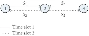
2.3. Physical-Layer Network Coding (PNC). We now intro-duce PNC as shown inFigure 4. Let us assume that the use of BPSK modulation at all the nodes. We further assume symbol-level time and carrier-phase synchronization, and the use of power control, so that the frames from N1 and N3arrive atN2 with the same phase and amplitude (Power control can be achieved in a slow fading channel with current techniques. Additional discussion about carrier-phase and symbol time synchronization can be found in [26]) . The
3 2
1
S1
S2
S3
S2
Time slot 1 Time slot 2
Figure4: Physical-layer network coding.
combined bandpass signal received byN2during one symbol period is
r2(t)=s1(t) +s3(t)
=a1cos(ωt) +a3cos(ωt)
=(a1+a3) cos(ωt),
(3)
wheresi(t),i=1 or 3, is the bandpass signal transmitted by
Ni,r2(t) is the bandpass signal received byN2 during one symbol period,ai is the BPSK modulated information bit
ofNi, and ωis the carrier frequency. Then,N2will obtain a baseband signala1+a3.
Note thatN2 cannot extract the individual information transmitted by N1 and N3, that is, a1 and a3, from the combined signal ina1+a3. However,N2is just a relay node. As long as N2 can transmit the necessary information to N1andN3 for extraction ofa1anda3 over there, the end-to-end delivery of information will be successful. For this, all we need is a special modulation/demodulation mapping scheme, referred to as PNC mapping in this paper, to obtain the equivalence of GF(2) summation of bits fromN1andN3 at the physical-layer.
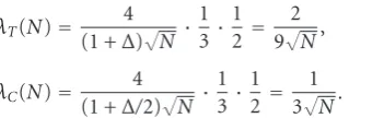
Table 1illustrates the idea of PNC mapping. InTable 1, sj ∈ {0, 1}is a variable representing the data bit ofNj and
aj∈ {−1, 1}is a variable representing the BPSK modulated
bit ofsjsuch thataj=2sj−1.
With reference to Table 1, N2 obtains the information bits:
s2=s1⊕s3. (4)
It then transmits
s2(t)=a2cos(ωt). (5)
The BER analysis in [6] shows that the end-to-end BER for the three schemes is similar when the per-hop BER is low (the BER is less than 10−5 for 10 dB). Ignoring the slight BER difference, we have the following conclusion. For a frame exchange, PNC requires two time slots, 802.11 requires four, while straightforward network coding requires three. Therefore, PNC can improve the system throughput of the three-node wireless network by a factor of 100% and 50% relative to traditional transmission scheduling and straightforward network coding, respectively.
3. Applying PNC in Regular 1D Networks
Table1: PNC Mapping: modulation mapping atN1,N2; demodulation and modulation mappings atN3.
Modulation mapping atN1andN3 Demodulation mapping atN2
Input Output
Input Output Modulation mapping atN2
Input Output
we discuss the application of PNC in 1D regular networks. There are two reasons for this discussion. First, the schemes proposed in regular network still work in random networks. And the analytical results in regular networks also provide some insights about applying PNC in random networks. Second, the regular network can also find applications in real world. For example, APs (access points) positioned along a highway form a regular linear chain in a vehicular network.
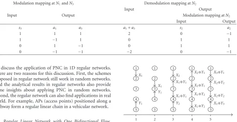
3.1. Regular Linear Network with One Bidirectional Flow. Consider a regular linear network withNnodes with equal spacing between adjacent nodes. Label the nodes as node 1, node 2,. . ., nodeN, successively with nodes 1 andNbeing the two source and destination nodes, respectively.Figure 5
shows a network with N = 5. Suppose that node 1 is to transmit frames X1,X2,. . . .to nodeN, and node N is to transmit framesY1,Y2,. . . .to node 1.
We could divide the time slots into two types: odd slots and even slots. In the odd time slots, the odd-numbered nodes transmit and the even-numbered nodes receive. In the even time slots, the even-numbered nodes transmit and the odd-numbered nodes receive.
Figure 5shows the sequence of frames being transmitted by the nodes in a 5-node network. In slot 1, node 1 transmits X1to node 2 and node 5 transmitsY1to node 4 at the same time. In slot 2, node 2 and node 4 transmitX1andY1to node 3 simultaneously; both node 2 and node 4 also store a copy ofX1 andY1 in their buffer, respectively. In slot 3, node 1 transmitsX2to node 2, node 5 transmitsY2to node 4, and node 3 broadcastsX1⊕Y1 simultaneously; node 3 stores a copy ofX1⊕Y1in its buffer. Adding the storedX1toX2⊕X1⊕
With reference to Figure 5, we see that a relay node forwards two frames, one in each direction, every two time slots. So, the throughput is 0.5 frame/time slot in each direction. Due to the half duplex assumption, this is the maximum possible throughput we can achieve.
As detailed above, when applying PNC on the linear network, each node transmits and receives alternately in successive time slots; and when a node transmits, its adjacent
Time slots
Figure5: Bidirection PNC transmission in linear network.
nodes receive, and vice versa (seeFigure 5). Let us investigate the signal-to-inference ratio (SIR) given this transmission pattern to make sure that it is not excessive. Consider the worst-case scenario of an infinite chain. We note the following characteristics of PNC from a receiving node’s point of view.
(a) The interfering nodes are symmetric on both sides. (b) The simultaneous signals received from the two
adjacent nodes do not interfere due to the nature of PNC.
(c) The nodes that are two hops away are also receiving at the same time, and therefore will not interfere with the node.
Therefore, the two nearest interfering nodes are three hops away. We have the following SIR:
SIR= P0/dα
2∗∞l=1P0/[(2l+ 1)d]α
, (6)
Table2: Signal to Noise Ratio with different path loss exponent
α 2 3 4 5 6
SIR (dB) 3.3 9.8 15.3 20.4 25.4
negligible for BPSK based on [28] (the capture threshold is often set to 10 db in wireless networks [3]). More generally, a thorough treatment should take into account the actual modulation scheme used, the difference between the effects of interference and noise, and whether or not channel coding is used. However, we can conclude that as far as the SIR is concerned, PNC is not worse thantraditional scheduling(see
Section 4) when generalized to then-node linear network (In this paper, we assume that channel coding [17] is properly used at all the nodes and the packets can be correctly decoded to avoid error propagation once the targeted SIR is achieved. Reference [17] provides and investigates a hop-to-hop channel coding scheme for PNC) .
3.2. Regular Linear Network with Multiple Flows. Part A considers only one bidirectional flow. Here we consider a general setting in which there are K unidirectional flows in theN-node linear network. Note that this generalization includes the scenario in which there is a combination of unidirectional and bidirectional flows in the network, since each bidirectional flow can be considered as two unidirectional flows.
To allow PNC to be applied, we compose bidirectional flows out of theKunidirectional flows by matching pairs of unidirectional flows in opposite directions. The bidirectional flows can then make use of PNC for transmission, while the remaining unmatched unidirectional flows make use of the traditional strategy of multihop data transmission.
The optimal way to compose the bidirectional flows and schedule the transmission of the links in the flows is a tough problem. Here we consider a simple heuristic which is asymptotically optimal for the regularN-node linear network when N goes to infinity as shown in Part C.For simplicity, we assume that all flows have equal traffic.
We define the following terms with respect to the linear network. Let us label the nodes from left to right by 1 toN sequentially. Let (si,di) denote the source-destination pair of
flowi. For a right-bound flow,si< di; for a left-bound flow,
si> di. LetFdenote the overall set of flows, andFR⊆Fbe the
set of right-bound flows andFL⊆Fbe the set of left-found
flows.
Two right-bound (left-bound) flowsiandjare said to be nonoverlapping ifdi < sj ordj < si (si < dj orsj < di). A
right packing(left packing) is a set of nonoverlapping right-bound flows (left-right-bound flows). A dual packing consists of a right packing and a left packing.Figure 6shows an example of a dual packing. Flows 2 and 3 form a right packing, and Flow 1 forms a left packing. Note that some of the nodes are traversed by both a right-bound flow and a left-bound flow. Let us call these nodes the common nodes, and the other nodes the noncommon nodes. A sequence of adjacent common nodes, flanked by but not including
Flow 1
Flow 2 Flow 3
Figure6: An example of a dual packing formed by a right packing and a left packing. An ellipse corresponds to a PNC unit. The nodes between two adjacent ellipses (including the terminal nodes of the ellipses) are grouped together by a rectangle.
two noncommon nodes at two ends (an ellipse inFigure 6), forms aPNC unit, and we can use the PNC mechanism for transporting the bidirectional traffic over it. A sequence of adjacent noncommon nodes, together with the two common nodes flanking them (a rectangle inFigure 6), may or may not have traffic flowing over them. When there is traffic, the traffic is in one direction only, and the traditional multihop communication technique can be used to carry the unidirectional traffic. Essentially, by forming a dual packing, we also form many “virtual” bidirectional flows (each corresponding to a PNC unit) on which PNC can be applied.
Our heuristic as showing in Algorithm 1 consists of a method of forming dual packings from theKunidirectional flows.
The dual packings yield a set of “virtual” bidirectional flows, each corresponding to a PNC unit. Scheduling can then be performed as follows. Let us refer to the time needed for all theKunidirectional flows to transfer one packet from source to destination as oneframe.Each link (hop) of a flow is allocated one time slot for transmission within a frame. A frame is further divided into two intervals, as follows.
(1) The first interval is dedicated to the PNC units (i.e., ellipses). Note that if there areMdual packings, 2M time slots are needed in the worst case; in the worst case, different dual packings use different time slots to transmit, and 2 time slots are needed for each dual packing (Two caveats are in order. The first is that according to our construction, there could be “trivial” PNC units with two nodes only. In this case, the PNC mechanism is not needed, and each node gets to transmit directly to the other node. Regardless of whether the PNC unit is trivial or not, two time slots are needed for the bidirectional flows. The second caveat is that there could be two PNC units in the same dual packing next to each other. For example, suppose nodes 1, 2, and 3 form a PNC unit, and nodes 4, 5, 6 form another. To avoid conflict, the scheduling of the transmissions on these two PNC units should be such that nodes 1, 3, 4, and 6 transmit in one time slot while nodes 2 and 5 transmit in another time slot. Again, two time slots are needed.).
while (F /= ∅){/∗Each iteration in the while loop forms a dual packing.∗/
while (FR= ∅)/ {/∗Each iteration in the while loop tries to find a “tight” right packing∗/
largestDest=0; while (true){
/∗Each iteration in the while loop includes one more flow into the right packing being assembled.∗/
i=arg minj∈FR:sj>largestDestsj
/∗Select a flow with the smallest source larger than LargestDest; assume “null” is returned if there is no more flow
left inFRwithsj>largestDest.∗/
if (i=null)/ {
include flowiinto the current right packing being assembled; largestDest=di;
remove flowifromF; }else
break;
/∗Break out of the while(true) loop.∗/ }
}
while (FL= ∅)/ {
/∗Each iteration in the while loop tries to find a “tight” left packing.∗/
/∗Comment: details omitted here; the procedure is similar to the “while (F
R= ∅)” loop above/
except that largestDest is replaced by smallestDest;sj>largestDest is replaced bysj<smallestDest etc.∗/
}
/∗Combine the right packings and left packings one by one to obtain dual packings∗/
}
Algorithm1
The number of time slots needed in the second interval depends on both the number and the lengths of the rec-tangles. As will be shown in Part C, it can be ignored compared to the time slots needed in the first interval asN goes to infinity.
3.3. Throughput of 1D Network with PNC. We now show that the packing and scheduling strategies presented in Part B can allow the upper-bound capacity of 1D network to be approached when the number of nodes N goes to infinity. Furthermore, compared with the conventional schemes discussed in [29], PNC can achieve a constant factor of throughput improvement.
We first detail the system model. To avoid edge effects, we consider a “large” circle instead of a line. TheNnodes are uniformly distributed over the circle with a constant distance between adjacent nodes. Without loss of generality, let the distance between two adjacent nodes be a unit distance. Each transmission is over only one unit distance (i.e., a node only transmits to its two adjacent nodes). Consider the receiver of a link. We assume that simultaneous transmission by another link whose transmitter is two or more hops away from the receiver of the first link will not cause a collision to the first link. In our model, N/2 nodes are randomly chosen as the source nodes. The remaining N/2 nodes are the potential destination nodes. For each source node, a unique destination node is chosen among the N/2 poten-tial destination nodes with equal probability. We assume matching without replacement in that the destination node chosen for a source node will not be put back to the pool before the destination node of another source is chosen. The
route for a source-destination pair is also predetermined in a random way (note: there are two routes from a source to its destination, one in the clockwise direction and the other in the counterclockwise direction).
The analytical results for the traditional transmission scheme and straightforward network coding scheme in our circular model are similar to those in the 1D linear network in [29] whenNgoes to infinity. Using similar approach, it is not difficult to obtain the respective per-flow throughputs in our circular network as
λT(N)= 2
N, λS(N)= 8
3N, (7)
where unit link bandwidth is assumed.
Let us now focus on the PNC throughput. We will show that PNC can achieve the per-flow throughput 4/N−εfor any small positive valueεasN goes to infinity. Let us first provide further details to the scheduling strategy presented in Part B.
above clockwise unidirectional packing, we form a matching counterclockwise unidirectional packing at choosingeas the start point and s as the end point. If there is an existing counterclockwise flow witheas its source node, we will start with this flow in the unidirectional packing. If not, we will choose the next flow with source node closest to e in the counterclockwise direction in our packing.
For “traffic balance”, after getting the first dual packing as above, for the next dual packing, we will start with forming the counterclockwise unidirectional packing first (i.e.,sande will be defined with respect to the counterclockwise packing) before constructing the matching clockwise packing. Repeat-ing the above procedure allows us to form a series of dual packings.
The scheduling of transmissions is the same as that in Part B except that here we also have to consider the transmission across the two subflows cut as above, if any. We assume the traffic from the destination of a preceding subflow to the source of its corresponding subflow is transmitted using the conventional scheme in the second interval.
With the above packing and scheduling strategies, we have the following theorem on the per-flow throughput of the 1D circular network whenNgoes to infinity.
Theorem 1. With PNC, we can approach the upper bound of the per-flow throughput of the 1D network:
λP(N)=
4
N. (8)
Sketch of Proof. A sketch of the proof for Theorem 1 is provided here and a detailed proof is given in the Appendix. With the help of the max-flow min-cut theorem, the upper bound of the per-flow throughput for our 1D circular network can be shown to be 4/N. That this upper bound can be approached with the application of the aforementioned PNC packing and scheduling strategies is argued as follows. Consider the originalN/4 unidirectional flows. With PNC packing and scheduling, these flows have been decomposed into PNC units and nonPNC units for transmission in the first and second intervals. For each round of first and second intervals (i.e., for each frame), one packet is transported from the source to the destination of each flow. We can show that the number of time slots needed in the first interval for all the flows is at most (1 +ε1)N/4, where the small positive quantityε1goes to zero asNgoes to infinity. The number of time slots needed in the second interval, on the other hand, isε2N, where the small positive quantityε2goes to zero asN goes to infinity. Then we can obtain the per-flow throughput with PNC: 1/(N/4 +ε1N/4 +ε2N/4)=(1−ε)N/4.
A corollary ofTheorem 1is that PNC can improve the throughput of the 1D network by a factor of 2 and 1.5 relative to the traditional transmission scheme and the SNC scheme (7), respectively.
A notable fact is that PNC can approach the capacity with minimum energy. Recall that PNC exchanges one packet between the two end nodes within two time slots, during which each of thennodes on the chain transmits once with
energy Et and receives once with energy Er. And a total
energyn(Et+Er) is used. In fact,n(Et+Er) is the lower bound
of energy to exchange one packet. For one exchange, the two end nodes must transmit once to send their message and must receive once to obtain their needed message; then−2 relay nodes must receive once and transmit once to finish one relay. Therefore, the energy ofn(Et+Er) is necessary.
4. Applying PNC in 2D Grid Network
Section 3focused on the 1D regular network. This section
investigates the application of PNC in a 2D regular gird network. We assume the same transmission protocol as in
Section 3.
4.1. 2D Grid Network with One Bidirectional Flow in Each
Line. Figure 7shows the grid network under consideration,
in whichN nodes are uniformly located at the cross points as shown. In this part, we first consider the case in which each line (horizontal or vertical) on the grid has one and only one bidirectional flow. Specifically, the two end nodes in each line, node 1 and node√N, exchange information through the relay nodes in between.
The flows transmit with the following PNC schedule. Consider the horizontal lines (similar schedule applies for the vertical lines). The first two time slots are dedicated to transmissions on lines 1,J+ 1, 2J+ 1,. . .; the next two time slots are dedicated to transmissions on lines nodes on the lines 2,J+ 2, 2J+ 2,. . .; and so on. The separationJmust be large enough for acceptable SIR. In the example ofFigure 7, J=4.
For a group of simultaneous active lines, to reduce SIR, when the odd nodes transmit on one active line, then the even nodes will transmit on its two adjacent active lines, as shown inFigure 7.
Let us investigate the SIR of this transmission pattern given a J. Consider the worst-case scenario in which N goes to infinity. For a given receiver, the interference from the nodes within the same line is I1 = 2∗
∞
l=1P0/[(2l+ 1)d]α, where P0, l, d = 1, and α are defined similarly as in Section 3.1. Without loss of generality, suppose that the receiver is an even node. The interference from the other active lines whose odd nodes are transmitting is I2 = 4
∞
k=0
∞
l=0P0/[(2l)2d2 +J2(2k + 2)2d2]α/2, and the interference from the other active lines whose even nodes are transmitting is I3 = 4
. Thus, the overall SIR is given by
SIR= P0/dα I1+I2+I3.
(9)
For a typical value ofα=4, the SIR in (9) is about 13.5 dB, 12.3 dB, and 10.0 dB for J equals 5, 4, and 3, respectively. With an assumed 10 dB target,J=3 is enough to guarantee successful transmission.
√ N
3 2 1 2 3
√ N
(a)
√ N
3 2 1 2 3
√ N
(b)
Figure7: Subfigure (a) shows 2D grid network with one bidirectional flow in each line. The lines separated byJ−1=3 lines, that is, the lines with the same color, are allowed to transmit simultaneously. Subfigure (b) shows a scheduling for one group active lines (red lines) in a specific time slot
Figure 7, we now randomly chooseN/2 of the nodes as the
source nodes. The remainingN/2 nodes are the destination nodes.
Here we apply a simple routing scheme, as in [29]. For a source-destination pair at positions (xs,ys) and (xd,yd), the
data will first be forwarded vertically to the node at (xs,yd)
before being forwarded horizontally to the destination. The horizontal and vertical transmissions are separated into two different time intervals. For horizontal (or vertical) transmissions, the scheduling within each line (column) is the same as that in theSection 3.2and the scheduling among different lines (columns) is the same as in part A.
WhenN goes to infinity, the number of nodes in each line or column,√N, also goes to infinity, and the per-flow PNC throughput in each line or column will approach 4/√N, as argued in Section 3. Since the horizontal transmission and vertical transmission are scheduled in different time interval and in each interval everyJlines (columns) transmit simultaneously, the per-flow transmission of PNC in the 2D grid network can approach
λP(N)=√4
N· 1 J ·
1 2 =
2
J√N. (10)
For comparison purposes, let us look at the per-flow throughput under the traditional transmission strategy and under the straightforward network coding strategy. With the routing/scheduling strategy and the corresponding throughput analysis in [29], we can show that the traditional transmission scheme and SNC scheme can achieve the following throughputs, respectively:
λT(N)= 4
(1 +Δ)√N· 1 3·
1 2 =
2 9√N,
λC(N)=
4 (1 +Δ/2)√N ·
1 3·
1 2 =
1 3√N.
(11)
In the 2D grid network, the nodes are tightly packed than in the 1D network, and the interfering nodes must be kept
at least 3 hops away, that is, Δ = 2, to obtain an SIR of no less than 10 dB (note: in the 1D network,Δcould be 1 for SIR of about 10 dB). When Δ = 2, we can verify that throughputs better than (11) cannot be achieved. In other words, the throughput in (11) is also the upper bound for traditional transmission scheme and SNC scheme under all possible schedulings.
Therefore, setting J = 3 in (10), we conclude that PNC can achieve a throughput improvement factor of 3 and 2 relative to the traditional transmission scheme and the SNC scheme, respectively. Note that the improvement factors under the 2D network are larger than those under the 1D network, which are 2 and 1.5, respectively (seeSection 3).
5. Conclusion
This paper has introduced a novel scheme called Physical-layer Network Coding (PNC) that significantly enhances the throughput performance of multihop wireless networks. Instead of avoiding interference caused by simultaneous elec-tromagnetic waves transmitted from multiple sources, PNC embraces interference to effect network-coding operation directly from physical-layer signal modulation and demod-ulation. With PNC, signal scrambling due to interference, which causes packet collisions in the MAC layer protocol of traditional wireless networks (e.g., IEEE 802.11), can be eliminated.
Appendix
A. Proof of
Theorem 1
This appendix proves Theorem 1 in three steps. First, the fact that 4/N is the upper bound for the throughput of the 1D circular linear network can be argued as follows. Let us consider the number of time slots needed so that each flow can transport one packet from its source to its destination. Due to half-duplexity, there can be at most N/2 transmitting nodes in a time slot. In general, each transmitting node can transmit to at most two of its adjacent nodes simultaneously. Hence, in total, there can be at most N one-hop transmissions being successfully completed in each time slot. The number of hops between the source and destination of a flow is on average N/2. There are altogetherN/2 flows. Using Chernoffbound, we can show that the total number of one-hop transmissions required (aggregated over all flows) is N2/4 w.h.p. as N goes to infinity. Thus, the time slots needed are lower bounded by (N2/4)/N = N/4. Within this number of time slots, each flow transports a packet from source to destina-tion. Thus, the per-flow throughput is upper bounded by λ≤1/(N/4)=4/N.
Next, we prove that the number of time slots needed in the second interval is negligible compared to N, denoted by ε2N where ε2 is a small positive quantity that goes to zero asNgoes to infinity. The total one-hop transmissions in the second interval can be divided into two parts, the one-hop transmissions in the rectangles and the one-hop transmissions between subflows (created when we unwrap the circular network into a linear network).
Let us first consider the rectangles. As shown inFigure 8, within a dual packing, the rectangles do not overlap. Furthermore, the two end nodes in a rectangle must be either a source or destination node of some flow. As a proof technique, let us artificially divide the rectangles into two groups according to the dual packings containing them. Recall that the dual packings are formed successively in our packing algorithm. Consider the first (1 − ε3) fraction of all flows (including the original flows and the generated subflows) that are included successively into the dual packings. The first group of rectangles arises from these flows. The second group of rectangles belongs to the remaining ε3 fraction of the flows. We set ε3 such that ε3=1/
logN.
As discussed inSection 3.2, when we perform packing on the circular network by unwrapping it to a linear network, it is possible for a flow to be cut into two subflows. Each clockwise unidirectional packing contains at least one flow that does not generate subflows (a flow cannot have more than N hops). As a corollary, if the clockwise packing contains a flow that has been cut into two subflows, then the packing must contain at least two flows to start with. One of these subflows will be relegated to a future packing exercise. So, each clockwise packing reduces the number of remaining flows to be packed by at least one. For the matching counterclockwise packing, at most one flow will be cut into two subflows. Thus, the matching counterclockwise
packing does not increase the number of remaining counter-clockwise flow. Recall from the discussion in Section 3.2
that for “traffic balance” successive dual packings will start with clockwise and counterclockwise packings in an alternate manner. Thus, successive dual packings will reduce the numbers of remaining clockwise and counterclockwise flows by at least one alternately.
In the beginning, there are N/2 original flows (N/4 of which are clockwise andN/4 of which are counterclockwise flows). From the argument in the previous paragraph, there are altogether at mostN/2 dual packings. Each dual packing will at most generate at most two extra flows to the flow pool (because of cut betweensande). Thus, altogether there could be at mostNextra flows being generated. Hence, the total number of flows (including the original flows and the subflows) is 3N/2.
In general, since the two end nodes of a rectangle must be either a source or a destination of some flow, the number of rectangles in a dual packing is no more than the number of flows in that dual packing (note: some nonend nodes within a rectangle could also be sources or destinations; thus the “no more than” rather than “equal to”). Therefore, the number of rectangles in the first group is no more than (1−ε3)N. For these rectangles, as shown inLemma 2at the end of this appendix, the number of nodes in each group-1 rectangle is no more than (1−ε4) log(N) +ε4Nw.h.p., whereε4is a small positive quantity that goes to zero whenN goes to infinity. Similarly, the number of rectangles in the second group is upper bounded byε3N. As a trivial bound, we will upper-bound the number of nodes in each group-2 rectangle by N. Note that each node will at most transmit once within a rectangle (group-1 or group-2) for traffic forwarding. Thus, the total number of one-hop transmissions needed for the rectangles is upper bounded by
T1=(1−ε3)N·
(1−ε4) log(N) +ε4N
+ε3N·N. (A.1)
Now, consider the transmissions across subflows. A one-hop transmission is needed for two adjacent subflows generated by the cut when we unwrap the circular network to a corresponding linear network. In other words, there is a one-hop transmission whenever there is an extra subflow, which is upper bounded by N/2 according to the above argument. Thus, the total number of one-hop transmis-sions between all adjacent subflows is upper bounded by T2=N/2.
are upper bounded by
k2=T1 +T2 N/2
=(1−ε3)N·
(1−ε4) log(N) +ε4N
+ε3N·N+N/2 N/2
=2(1−ε3)(1−ε4) log(N) + 2(1−ε3)ε4N+ε3N+ 1
=Nε2,
(A.2)
whereε2is determined byε3,ε4, andN. It is easy to show that ε2will go to zero asNgoes to infinity.
Finally, we prove that the number of time slots needed in the first interval is less than (1 +ε1)N/4. In a unidirectional packing, a residual node is an idle node that through which no packet passes (i.e., none of the flows of the unidirectional packing passes through the node). Thus, the number of nodes through which one packet passes in one unidirectional packing isN, minus the number of residual nodes. Consider a dual packing to which group-1 rectangles belong. According toLemma 1immediately after the proof ofTheorem 1here, the number of residual nodes in each of the unidirectional packings of the dual packings is less than log(N) w.h.p.. That is, the number of nonresidual nodes in a unidirectional packing is more thanN-log(N) w.h.p., and the number of nonresidual nodes in both the unidirectional packings of the dual packing is more than 2(N −logN). That is, the traffic handled by each dual packing (in terms of packet flows across all nodes in the dual packing) is more than 2(N−logN).
Now, consider an arbitrary node in the network. Accord-ing to our model, it is either the source or destination of some flow. The packet of that flow passes through it with probability 1. For the otherN/2 −1 original flows, a packet passes through the node with probability 1/2. By the Chernoff-Hoeffding theorem, the number of packets that go through each node is 1/2·(N/2−1) + 1 w.h.p.. Considering allNnodes, the number of packets passing through them is (1/2(N/2−1) + 1)N. Note that this is the total traffic which is more than the traffic in the dual packings to which group-1 rectangles belong.
Therefore, the number of dual packings to which the group-1 rectangles belong is upper bounded by
(1/2(N/2 −1) + 1)N
2N−log(N) w.h.p. (A.3)
Similar to the argument for group-1 rectangles, for the flows containing the group-2 rectangles, there are at most ε3N flows which will generate at most ε3N unidirectional packings, that is,ε3N/2 dual packings. Then we can obtain that the total number of dual packings is no more than
(1/2(N/2 −1) + 1)N 2N−log(N) +
ε3N
2 =
(1 +ε1)N
8 , (A.4)
with high probability, whereε1is determined byε3 andN. It is easy to verify thatε1goes to zero asNgoes to infinity.
Since each packing needs at most two times slots, the time slots needed for the first interval are at mostk1=(1+ε1)N/4. With the help ofk1andk2, we can obtain the lower bound of the per-flow throughput as
λP(N)= 1
k1+k2
= 1
(1 +ε1)N/4 + 2 log(N) + 2Nε2+ 1
= 4 N
1
1 +ε1+ 2 log(N)/N+ 2ε2+ 1/N = 4 N(1−ε),
(A.5)
whereεcan be obtained fromε1,ε2, andN, and it goes to zero asNgoes to infinity. ThenTheorem 1is proved.
Lemma 1. For any clockwise (counterclockwise) unidirectional packing contained in the dual packings to which group-1 rectangles belong, the number of residual nodes is less than log(N)w.h.p.
Proof. LetPdenote the set of dual packings to which group-1 rectangles belong. Let us focus on one clockwise unidirec-tional packing p inP. The proof for the counterclockwise case is similar. LetPcbe the clockwise packings inP. Letm
denote the number of clockwise flows in Pc. According to
our way of partitioning the rectangles into the two groups, we havem ≤ (1−ε3)N1, whereN1 is the total number of clockwise flows.
Recall that in our traffic model, we randomly selectN/2 nodes to be sources and N/2 nodes to be destinations. In other words, any node among theNnodes is either a source or a destination. This applies to any residual node inpas well. In particular, a residual node inpis either (1) a destination node (of a clockwise or counter-clockwise flow), (2) a source node of a counter-clockwise flow, or (3) a source node of a clockwise flow. In case 3, since the residual node is a residual node in p, it must be a source node of a clockwise flow already packed (i.e., already belong toPc) prior to packing
p.
For a unidirectional packing, consider the first flow from the start point s. Suppose this flow ends at nodei. Let us consider the probability of node (i+ 1) being a residual node with respect to this unidirectional packing. Due to the randomness of our packing procedure and our random selection of sources and destinations for flows, node (i+ 1) is a destination node with probabilityp1=1/2; it is a source node of a counter-clockwise flow with probabilityp2 =1/4 w.h.p, and it is a source node of a prepacked clockwise flow with probabilityp3≤(1−ε3)/4 w.h.p. Then the probability that node (i+ 1) is a residual node given that nodeiis not a residual node is
P(1|0)=p1+p2+p3≤1−ε3
4. (A.6)
Flow 1 Flow 2
Flow 3 Flow 4
Figure8: An example of a dual packing, where flow 1 and flow 2 belong to the clockwise unidirectional packing, flow 3 and flow 4 belong to the counterclockwise unidirectional packing. The white nodes are nonresidual nodes, the red nodes are the residual nodes of the clockwise unidirectional packing, the green nodes are the residual nodes of the counterclockwise packing, and the blue nodes are the residual nodes of both the two unidirectional packings. The nodes in the rectangles are the uncommon nodes.
Given node (i+ 1) is a residual node, the probability that the node (i+ 2) is also a residual node isP(2 | 1) ≤ P(1| 0) (due to sampling without replacement). The probability of a sequence oflor more residual nodes is given by
P(1|0)P(2|1)P(3|2)· · ·P(l|l−1)≤[P(1|0)]l
≤
1−ε3 4
l
. (A.7)
When l = log(N), as N-goes to infinity, the above probability is exp(−log(N)/4), which will approach zero. Thus,Lemma 1is proved.
Lemma 2. For group-1 rectangles, the number of nodes in each rectangle is no more than 2log(N)with probability1−ε4, where ε4is a small positive quantity that goes to zero when N goes to infinity.
Proof. With respect to Figure 8 and the explanation in its caption, letNr,Ng,Nbdenote the number of red, green, and
blue nodes in a dual packing, respectively. By Lemma 1, Nr +Nb ≤ log(N), and Ng +Nb ≤ log(N) w.h.p. Thus,
Nr+Ng+Nb≤Nr+Ng+ 2Nb≤2 log(N).
Acknowledgments
This work was partially supported by the Competitive Ear-marked Research Grant (project number 414507) established under the University Grant Committee of the Hong Kong and the Natural Science Foundation of China (project number 60902016).
References
[1] T. Ojanper¨a and R. Prasad, “An overview of air interface multiple access for IMT-2000/UMTS,”IEEE Communications Magazine, vol. 36, no. 9, pp. 82–95, 1998.
[2] J. Li, C. Blake, D. S. J. De Couto, H. I. Lee, and R. Morris, “Capacity of ad hoc wireless networks,” inProceedings of the 7th Annual International Conference on Mobile Computing and Networking (MOBICOM ’01), pp. 61–69, Rome, Italy, July 2001.
[3] P. C. Ng and S. C. Liew, “Throughput analysis of IEEE802.11 multi-hop ad hoc networks,” IEEE/ACM Transactions on Networking, vol. 15, no. 2, pp. 309–322, 2007.
[4] R. Ahlswede, N. Cai, S.-Y. R. Li, and R. W. Yeung, “Network information flow,”IEEE Transactions on Information Theory, vol. 46, no. 4, pp. 1204–1216, 2000.
[5] S.-Y. R. Li, R. W. Yeung, and N. Cai, “Linear network coding,”
IEEE Transactions on Information Theory, vol. 49, no. 2, pp. 371–381, 2003.
[6] S. Zhang, S. C. Liew, and P. P. Lam, “Hot topic: physical-layer network coding,” in Proceedings of the 12th Annual International Conference on Mobile Computing and Networking (MOBICOM ’06), pp. 358–365, Los Angeles, Calif, USA, September 2006.
[7] P. Popovski and H. Yomo, “The anti-packets can increase the achievable throughput of a wireless multi-hop network,” in
Proceedings of IEEE International Conference on Communica-tions (ICC ’06), vol. 9, pp. 3885–3890, Istanbul, Turkey, July 2006.
[8] Y. Hao, D. Goeckel, Z. Ding, D. Towsley, and K. K. Leung, “Achievable rates for network coding on the exchange channel,” in Proceedings of IEEE Military Communications Conference (MILCOM ’07), Orlando, Fla, USA, October 2007. [9] S. Katti, S. Gollakota, and D. Katabi, “Embracing wireless interference: analog network coding,” Tech. Rep. MIT-CSAIL-TR-2007-012, MIT, Cambridge, Mass, USA, 2007.
[10] M. Denkberg, “Paired carrier multiple access(PCMA) for satellite communications,” in Proceedings of the Pacafic Telecommunications Conference, Honolulu, Hawaii, USA, 1998.
[11] T. Cui, T. Ho, and J. Kliewer, “Memoryless relay strategies for two-way relay channels: performance analysis and opti-mization,” inProceedings of IEEE International Conference on Communications (ICC ’08), pp. 1139–1143, Beijing, China, May 2008.
[12] S. Zhang, S. C. Liew, and L. Lu, “Physical layer network coding schemes over finite and infinite fields,” inProceedings of IEEE Global Telecommunications Conference (GLOBECOM ’08), pp. 3784–3789, New Orleans, La, USA, November-December 2008.
[13] T. Koike-Akino, P. Popovski, and V. Tarokh, “Denoising maps and constellations for wireless network coding in two-way relaying systems,” inProceedings of IEEE Global Telecommu-nications Conference (GLOBECOM ’08), pp. 3790–3794, New Orleans, La, USA, November-December 2008.
[14] S. Zhang and S. Liew, “Capacity of two-way relay chan-nel,” 3rd HK-BJ Doctoral forum, 2008, http://arxiv.org/ ftp/arxiv/papers/0804/0804.3120.pdf.
[15] W. Nam, S.-Y. Chung, and Y. H. Lee, “Capacity bounds for two-way relay channels,” inProceedings of the International Zurich Seminar on Digital Communications (IZS ’08), pp. 144– 147, Zurich, Germany, March 2008.
[16] K. Narayanan, M. P. Wilson, and A. Sprintson, “Joint physical layer coding and network coding for bi-directional relaying,” in Proceedings of the 45th Annual Allerton Conference on Communication, Control, and Computing, Monticello, Ill, USA, September 2007.
[17] S. Zhang and S.-C. Liew, “Channel coding and decoding in a relay system operated with physical-layer network coding,”
IEEE Journal on Selected Areas in Communications, vol. 27, no. 5, pp. 788–796, 2009.
Journal on Selected Areas in Communications, vol. 27, no. 5, pp. 763–772, 2009.
[19] C. Chen, K. Cai, and H. Xiang, “Scalable ad hoc networks for arbitrary-cast: practical broadcast-relay transmission strategy leveraging physical-layer network coding,”EURASIP Journal on Wireless Communications and Networking, vol. 2008, Article ID 621703, 15 pages, 2008.
[20] Y. Wu, P. A. Chou, and S. Y. Kung, “Information exchange in wireless networks with network coding and physical layer broadcast,” Tech. Rep. MSR-TR-2004-78, Microsoft Research, Redmond, Wash, USA, 2004.
[21] C. Hausl and J. Hagenauer, “Iterative network and channel decoding for the two-way relay channel,” in Proceedings of IEEE International Conference on Communications (ICC ’06), vol. 4, pp. 1568–1573, Istanbul, Turkey, July 2006.
[22] J. N. Laneman, D. N. C. Tse, and G. W. Wornell, “Cooperative diversity in wireless networks: efficient protocols and outage behavior,”IEEE Transactions on Information Theory, vol. 50, no. 12, pp. 3062–3080, 2004.
[23] T. M. Cover and A. A. El-Gamal, “Capacity theorems for the relay channel,”IEEE Transactions on Information Theory, vol. 25, no. 5, pp. 572–584, 1979.
[24] L. Lai, K. Liu, and H. El-Gamal, “On the achievable rate of three-node wireless networks,” inProceedings of the IEEE Inter-national Conference on Wireless Networks, Communications and Mobile Computing, vol. 1, pp. 739–744, Maui, Hawaii, USA, June 2005.
[25] S. Katti, H. Rahul, W. Hu, D. Katabi, M. Medard, and J. Crowcroft, “XORs in the air: practical wireless network coding,”IEEE/ACM Transactions on Networking, vol. 16, no. 3, pp. 497–510, 2008.
[26] S. Zhang and S. Liew, “Synchronization analysis in phys-ical layer network coding,” Submitted, http://arxiv.org/ abs/1001.0069.
[27] T. S. Rappaport, Wireless Communications: Principles and Practice, Prentice-Hall, Englewood Cliffs, NJ, USA, 1996. [28] J. G. Proakis, Digital Communications, McGraw-Hill, New
York, NY, USA.