Simulation analysis of differential phase delay estimation
by same beam VLBI method
Fuyuhiko Kikuchi, Qinghui Liu, Koji Matsumoto, Hideo Hanada, and Nobuyuki Kawano
RISE Project Office, National Astronomical Observatory, 2-12 Hoshigaoka, Mizusawa-ku, Oshu, Iwate 023-0861, Japan
(Received February 23, 2007; Revised September 21, 2007; Accepted November 9, 2007; Online published April 9, 2008)
The same beam VLBI method (SBV) is newly applied to the multi-frequency VLBI method in the VRAD mission of SELENE (KAGUYA). By simultaneously observing two nearby spacecraft with one antenna, the error sources of VLBI measurement common in two propagation paths can be almost canceled out. In this paper, error estimation and simulation analysis are carried out for a feasibility study to apply the SBV method to the VRAD mission. Differential phase delay can be estimated without cycle ambiguity even if tropospheric fluctuation is large and/or traveling ionospheric disturbance occurs. The sensitivity of the differential phase delay with respect to the average elevation angle and the elongation of two spacecraft is also investigated. Moreover, a method is developed for estimating differential phase delay in switching VLBI observations using the cycle ambiguity derived from SBV observations. This method can be performed in more than 90% of the VRAD mission’s total paths. Precise positioning with SBV contributes to accurate estimation of the low degree coefficients of lunar gravity fields by more than one order of magnitude than previous results.
Key words:VLBI, spacecraft, orbit determination, narrow bandwidth, differential phase delay, VRAD, RSAT, SELENE (KAGUYA).
1.
Introduction
1.1 SELENE (KAGUYA)/VRAD mission
In the Japanese lunar explorer SELENE (KAGUYA) (SELenological and ENgineering Explorer), the Research In SElenodesy (RISE) group has studied the lunar gravity field (Kawano, 1997; Kawanoet al., 1998) by differential VLBI observations of the VRAD (differential VLBI radio sources) mission (Hanadaet al., 2002) and 2- and 4-way Doppler observations of the Relay SAtellite Transponder (RSAT) mission (Namikiet al., 1999) in addition to lunar topography observations of the Laser ALTimeter (LALT) mission (Arakiet al., 1999).
The VLBI technique has been applied to spacecraft track-ing since the 1960s (e.g., Border et al., 1992; Sagdeyev et al., 1992). VLBI observations of spacecraft have been used for deep space missions of NASA and ESA, for ex-ample, the orbit determination of Mars Odyssey during its interplanetary cruise (Antreasianet al., 2002; Thornton and Border, 2003). However, group delay accuracy was limited to several hundred pico-second (ps) due to the narrow span in the downlink signals from the spacecraft. The accuracy of group delay is not sufficient for precise lunar gravity field estimation. In order to estimate the low degree coefficients of lunar gravity fields by more than one order of magnitude than previous results, phase delay estimation whose accu-racy is expected to be several ps is needed (Hanadaet al., 2002).
Copyright cThe Society of Geomagnetism and Earth, Planetary and Space Sci-ences (SGEPSS); The Seismological Society of Japan; The Volcanological Society of Japan; The Geodetic Society of Japan; The Japanese Society for Planetary Sci-ences; TERRAPUB.
In the VRAD mission, two VLBI radio sources are loaded on two sub-satellites called Rstar and Vstar. These on-board radio sources transmit four carrier wave signals to carry out differential VLBI observations between Rstar and Vstar. The signals consist of three carrier wave signals in S-band (fs1 =2212 [MHz], fs2 =2218 [MHz], and fs3 =
2287 [MHz]) and one in X-band (fx1 =8456 [MHz]). The
frequencies of these signals are allocated to resolve the cycle ambiguity of the differential phase delay of the X-band signal using the multi-frequency VLBI (MFV) method (Konoet al., 2003). When conditions are completely sat-isfied for deriving the cycle ambiguity of the differential residual fringe phase (RFP), which is the difference of the residual fringe phase (RFP) between Rstar and Vstar, the differential phase delay of the X-band signal can be es-timated within error of 3.3 ps if the baseline length is as-sumed to be 2000 km (Konoet al., 2003). The differential phase delay is highly sensitive to the relative position and velocity of the two sub-satellites in the direction perpen-dicular to the line-of-sight (LOS). VRAD observations can contribute to estimate the gravity field of the limb region of the moon. After combining the Doppler observation in the RSAT mission, which is sensitive to the LOS direction, the spacecraft’s three-dimensional motion can be determined. In the processes of orbit determination and lunar gravity field estimation, the differential phase delay is converted to doubly differenced 1-way range as observable which is in-put to orbit determination software ‘GEODYN II’ (Pavliset al., 2001). The orbit determination process involves the ob-servation modeling consisting of calculation of station co-ordinates as well as orbital motion of the spacecraft with
respect to the lunar reference frame.
1.2 Application of same beam VLBI method for MFV
Three conditions must be satisfied to achieve differential phase delay estimation by the MFV method (Konoet al., 2003): First, the phase error of the RFP of the signals from two nearby spacecraft must be less than 4.3 degrees in the S-band and 179 degrees in the X-band signals. Second, the total electron content (TEC) of the ionosphere through which the propagation path from the spacecraft crosses must be corrected within error of 0.23 TECU (1 TECU is 1016 el/m2). Third, initial geometric delay, which is used in the correlation of the signal from the spacecraft, must be known within error of 83 nanoseconds (ns). The switching VLBI observation method was proposed to satisfy the con-ditions of the MFV method (Konoet al., 2003). By alter-nately observing two nearby spacecraft, some error sources of VLBI such as tropospheric fluctuation and ionospheric delay can be canceled. However, tropospheric fluctuations with a period shorter than the switching interval still re-main. Because the remaining tropospheric fluctuation is a flicker noise (Liu et al., 2005), phase error cannot be re-duced by the time integration ofRFP. For the TEC con-dition, GPS TEC observations near the VLBI station can be used to correct the ionospheric delay (Pinget al., 2002) as well as its cancellation by switching VLBI observation. However, when a traveling ionospheric disturbance (TID) occurs in the ionosphere (Afraimovichet al., 2000), satis-fying the TEC condition is difficult.
We solve this problem by applying the same beam VLBI method for differential phase delay estimation by the MFV method (Liuet al., 2007). When elongation between two nearby spacecraft becomes smaller than the beam width of the ground antenna, their signals can be simultaneously received. Most error sources are expected to be canceled out by applying this method. Although the same beam VLBI test observation was carried out in the 1980s (Border et al., 1992; Folkneret al., 1993), differential phase delay estimation without cycle ambiguity is applied for the first time.
This paper evaluates the error sources of differential phase delay in the same beam VLBI observation, especially for thermal noise, tropospheric delay, and ionospheric de-lay. The sensitivity of differential phase delay with respect to average elevation angle and elongation of the two space-craft is newly investigated. A new method is also described for correcting ionospheric delay.
All considerable error sources are evaluated by referring to the error estimation results in Liu et al.(2007). Based on those results, simulation analysis is carried out under the predicted conditions of the VRAD mission. The results of simulation analysis show that differential phase delay can be estimated without cycle ambiguity by the same beam VLBI method even if the tropospheric fluctuation is large and/or TID occurs.
2.
MFV Method
2.1 Description of differential residual fringe phase
Residual delay τ(t), which is the difference between the observed and the calculated delay time, can be
repre-sented as:
τ(t)=τgeo(t)+τinst(t)+τclock(t)
+τtrop(t)+τion(t), (1)
where τgeo(t) is the residual geometric delay and
τclock(t)is a clock offset, which is the difference between
the time references of each station. τinst(t), τtrop(t),
and τion(t) are the differences of the instrumental,
tro-pospheric, and ionospheric delays between the remote and reference stations. In these delays,τion(t)is proportional
to 1/f2 in contrast to the other delays that are almost
con-stant with respect to the frequency. The ionospheric delay is defined as (Pinget al., 2002):
τion(t)= −kD(t)/frf2, (2)
wherekis the constant (1.34×10⁻⁷ [m2s/el]), D(t)is
the TEC difference in the ionosphere along the propagation paths of each signal, and frf is the radio frequency of the
signal from the spacecraft. From Eqs. (1) and (2), RFP is written as:
φ(t)=2πfrfτ(t)
=2πfrfτ(t)−2πkD(t)/frf, (3)
where τ(t)=τ
geo(t)+τinst(t)+τclock(t)+τtrop(t). (4)
In addition, the RFP obtained from the correlation has a value between 0 and 2π and an ambiguity of 2πN where Nis the integer that represents its cycle ambiguity: Finally, RFP is written as:
φ(t)=2πfrfτ(t)−2πkD(t)/frf−2πN+σφ, (5)
whereσφis the phase error of RFP.
When the elongation of two radio sources is smaller than the beam width of the ground antenna for the corresponding frequency band, two radio sources can be observed simulta-neously. In cases of asame beamVLBI observation,RFP 2φ(t)is expressed as:
2φ(t)=φsource2(t)−φsource1(t)
=2πfrf(2τgeo(t)+2τtrop(t))
−2πk2D(t)/frf−2πN+σφ, (6)
where 2τ
geo(t)=τgeosource2(t)−τgeosource1(t) (7)
2τ
trop(t)=τtropsource2(t)−τ source1
trop (t) (8)
2D(t)=Dsource2(t)−Dsource1(t) (9)
N =Nsource2−Nsource1 (10)
σ
φ =
√
2σφ. (11)
2τ
geo(t)is the difference between the residual geometric
delays of two radio sources. 2τ
trop(t),2D(t), andN
Table 1. Conditions of MFV method for error sources of differential phase delay of X-band signal in VRAD mission.
2.2 Deriving cycle ambiguity
The three carrier wave signals in the S-band and one in the X-band are used to derive the differential phase delay of the X-band signal. TheRFP of each frequency signal is represented as: X-band signals, respectively.2τs
geoand2τ
x
geoare the
dif-ferences of the residual geometric delays of the two space-craft for the S-band and X-band signals because the phase and geometric centers of the S-band and X-band antennas are different in the VRAD mission. The differential phase delays of the S-band and X-band signals,2τ
s and2τx, are derived by the MFV method.
Cycle ambiguitiesNs2−Ns1,Ns3−Ns1,Ns1,
To uniquely derive the cycle ambiguities, the conditions shown in Table 1 must be satisfied (Kono et al., 2003). Moreover, the sum of the error sources from Eqs. (16) to (19) must be less than 0.5:
σs2−s1=
When all conditions described from Eqs. (20) to (23) and Table 1 are satisfied, differential phase delay 2τ
x of the X-band signal can be derived without cycle ambiguity:
2τ
3.
Application of Same Beam VLBI Method for
VRAD
3.1 Relation between beam width of ground antenna and elongation of two spacecraft in VRAD
0 2 4 6 8 10
0 7 14 21 28
Number of paths
Day Total number
Same beam VLBI
Fig. 1. Number of opportunities for same beam VLBI observation in VRAD mission.
power beam width of ground antennaθHPBWis represented
asλ/D, whereλis the wavelength of a radio signal andD is the diameter of a ground antenna. Therefore,θHPBW is
0.37 degrees for the S-band signal and 0.1 degrees for the X-band signal. When elongation between the two VRAD spacecraft is smaller than 0.1 degrees, the same beam VLBI observation can be carried out both in S- and X-band sig-nals. When elongation is between 0.1 and 0.37 degrees, it is larger than the beam width for the X-band signal. There-fore, switching VLBI observation is carried out in the X-band signal. In this case, same beam VLBI observation can only be conducted in the S-band signal. When elongation is larger than 0.37 degrees, switching VLBI observation is carried out both in the S- and X-band signals.
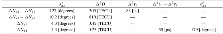
3.2 Rate of same beam VLBI observation to whole ob-servation period in VRAD
When there is at least one occasion of same beam VLBI observation in the continous observation path, differential phase delay can also be obtained in the period of the switch-ing VLBI by referrswitch-ing to that obtained in the period of the same beam VLBI described in Section 5.5. Therefore, the number of paths in which same beam VLBI observation can be carried out is estimated.
The result is shown in Fig. 1. This is an example of a one-month period. The orbital elements of the two spacecraft in the VRAD mission are shown in Table 2, where a is the semi-major Axis,eis the eccentricity, I is the orbital inclination,is the right ascension of the ascending node, ω is the argument of the perigee, and MA is the mean anomaly. The white column represents the total number of paths for each day. When the orbits of the two spacecraft around the moon keep face on the day, the total number of paths is 1. On the other hand, the total number of paths is more than 2 when occultation of the spacecraft by the moon occurs. The black column represents the number of paths in which same beam VLBI observation can be carried out. When the period of same beam VLBI observation continues for at least 50 seconds, this number is counted because the minimum integration period of RFP is 50 seconds for deriving its cycle ambiguity, as described in Section 4.1. This estimation is one example, and it would change by the day of the launch. However, this result is almost identical in any month. From Fig. 1, same beam VLBI observation can be carried out in 59% of the paths. This percentage can be improved by optimizing the observation schedule of the VRAD mission in which the observation period can
be selected relatively and flexibly. VLBI observation will be conducted three days a week, for a total of 24 hours of weekly observation. As a result of the optimization of the observation schedule, same beam VLBI observation can be planned for 90% of the observation paths in this estimation. In summary, there is sufficient opportunity for same beam VLBI observation to estimate the moon’s gravity field with desired accuracy (Matsumotoet al., 2007).
4.
Modeling of Error Sources in Same Beam VLBI
Observation
The error sources of differential phase delay in same beam VLBI observation are modeled by referring to the error estimation results (Liuet al., 2007). In the process of modeling, the effect of thermal noise, tropospheric delay, and ionospheric delay are newly evaluated.
4.1 Signal-to-noise ratio of cross spectrum
Thermal noise introduces a random fluctuation to RFP. The effect of thermal noise can be evaluated from the SNR of the cross spectrum of the correlated signals. The phase error of RFP is inversely proportional to SNR
σφ = 1
SNR . (25)
The frequency stability of the crystal oscillator, which is identical to VRAD’s at room temperature, has already been measured (Asariet al., 2001). Allan standard devia-tion (ASD) is about 6×10⁻¹⁰ at an average time of one
second, which is the minimum integration period of RFP. Frequency stabilityδf0/f is approximately represented as:
δf0
f =6×10
−10, (26)
where f is the radio frequency of the signal. For VRAD, δf0 predicted from this equation is 1.4 Hz at f =
2287 MHz, which is the highest frequency of the signals in S-band, and 5.1 Hz at f =8456 MHz in X-band.
In addition, the temperature change in the spacecraft af-fects the frequency stability. The specification of tempera-ture coefficientd f/d T of the crystal oscillator of VRAD is 1.375×10⁻⁷· f in the range of−25◦C to+55◦C (Asariet
al., 2001). Since the actual temperature change in the space-craft is not clear, it is assumed to be±20◦C based on the fol-lowing situation. When the spacecraft is in the sunlight for half of the orbital period, which averages about 1.5 hours (Matsumotoet al., 2007), the temperature linearly increases with time by 40 degrees from−20◦C to +20◦C. On the other hand, when the spacecraft is under an eclipse for the another half of the orbital period, the temperature linearly decreases with time by the same amount. Under these as-sumptions, the rate of the temporal change of temperature d T/dτ is 7.4×10⁻³◦C/s. The frequency stability caused by the temperature change in the spacecraft,δftemp/f, is
repre-sented as:
δftemp=d f/d T·d T/dτ ·τ, (27)
whereτ is the time scale of the frequency stability. Whenτ is one second,δftemppredicted from this equation is 2.3 Hz
Table 2. Orbital elements of Rstar/Vstar.
a[m] e I[deg.] [deg.] ω[deg.] MA[deg.]
Rstar 3004353.503 0.3678184689 89.76783829 120.1122954 146.2552392 335.6972982 Vstar 2197699.003 0.1394090403 89.66102628 120.0836218 143.7253249 162.7991062
Table 3. Summary of evaluation of C/N0of signals and SNR of cross spectrum.
C/N0 δfsum C/N √2fB SNR (1 s) σφ(1 s) σφ(50 s)
S-band 17.3 dB·Hz −6.1 dB Hz 11.2 dB +4.6 dB 15.7 dB 1.5 deg. 0.21 deg.
X-band 19.4 dB·Hz −11.8 dB Hz 7.6 dB +7.4 dB 15.0 dB 1.8 deg. 0.25 deg.
Moreover, the received frequency of the signal is changed by the Doppler shift. The frequency spectrum of the sig-nal is broadened and introduces a decrease of C/N0. For
VRAD, the maximum Doppler shift per second δfdop is
about 13 Hz/s in S-band and 50 Hz/s in X-band from the simulation results of this article. Doppler shift fdop(t)can
be compensated for by multiplying function e−2π·fdop(t) to
the time series of the received signal and calculated from the spacecraft’s velocity, whose accuracy is estimated to be less than 0.05 m/s in the VRAD mission. The Doppler shift can be compensated for within error of 0.4 Hz for S-band and 1.3 Hz for X-band.
From these results, sum δfsum of δf0, δftemp, δfdop is
4.1 Hz in S-band and 15 Hz in X-band. The decrease of C/N0is 6.1 dB Hz in S-band and 11.8 dB Hz in X-band. In
VLBI, SNR is expressed by the product of the C/N and the square root of the bandwidth of signal B that corresponds toδfsumin this case:
SNR=C/N·√2B. (28)
Therefore, SNR increases by 4.6 dB in S-band and 7.4 dB in X-band.
Finally, these results are summarized in Table 3. SNR can be improved by integrating RFP, which is proportional to the square root of the integration period. When the inte-gration period is assumed to be 50 seconds, the phase error of the S-band and X-band signals is 0.21 and 0.25 degrees, respectively, satisfying the MFV condition.
For simulation analysis of the differential phase delay estimation, thermal noise is modeled as purely white noise. Thermal noisenthermal(t)has Gaussian distribution in which the average value is 0 and the standard deviation isAthermal:
Athermal=
BS-RTP
C/N0 . (29)
The recording bandwidth of S-RTP BS-RTPis 100 kHz. In the simulation, the C/N0 obtained from the test
measure-ments in VRAD is 17.3 dB/Hz in S-band and 19.4 dB Hz in X-band signals.
4.2 Tropospheric delay
4.2.1 Average component of tropospheric delay
The error for the average component of tropospheric delay δτtropbecomes offset error of the differential phase delay
because separating geometric delay from tropospheric de-lay is difficult using the different frequency signals of the VRAD mission. The average component of tropospheric
10 20 30 40
50 6070 80 90 El [degree] 0
0.20.4 0.60.8
1
El [degree] 0
2 4 6 8 10 12 14
Error of tropospheric delay [ps]
Fig. 2. Error of average component of tropospheric delay.
delay is compensated for by the predicted tropospheric de-lay in the zenith angle at each ground station and the map-ping function (Niell, 1996). The error of dry zenith delay δτdry
zenithis about 3.3 ps under hydrostatic equilibrium
con-ditions (Niell, 1996). The error of the wet zenith delay δτwet
zenithestimated from GPS data is about 17 ps (Eloseguiet
al., 1998). In cases of differential VLBI observationsδτtrop caused by the differences of elevation angles between two spacecraft after correcting the dry and wet delays is repre-sented here as:
δτtrop=√2·δτz
dry·
mdry
El1
−mdry
El2
+√2·δτwetz ·
mwet
El1
−mwet
El2
(30)
El1=Elave+
El
2 ,El2=Elave− El
2 ,
whereElave andEl are the average and the difference of
the elevation angles of two spacecraft and mdry(El)and
mwet(El)are the mapping functions for the dry and wet
delays, respectively. The multiplication of √2 means the root sum square of the errors of the tropospheric delay generated at two VLBI stations.
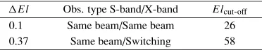
Figure 2 shows the error of the average component for tropospheric delay in each Elave andEl. For cases of
same beam VLBI observations both in S- and X-bands (in whichElis less than 0.1 degrees) and that for only in S-band (in whichEl is between 0.1 degrees and 0.37 de-grees), δτtrop is smaller than 2 ps when El
ave is larger
than 15 degrees. For cases of switching VLBI observation (in whichEl takes the maximum value of 0.9 degrees), δτtrop, which is 6 ps atEl
ave is 15 degrees. This error
Fig. 3. Frozen screen model.
4.2.2 Dynamic component of tropospheric delay
The dynamic component of tropospheric delay is caused by water vapor in the troposphere. Water vapor in the lower layer of the troposphere takes a large refractive in-dex and varies rapidly both temporally and spatially. It is well known that the statistical property of the tropospheric fluctuation is consistent with Kolmogorov turbulence (Liu et al., 2005).
When the density distribution of the water vapor is as-sumed to follow the Kolmogorov theorem, the dynamic component of the troposphere can be modeled as a “frozen screen”. In this model, water vapor exists in blocks of var-ious sizes that are moved by the wind while retaining their shapes. As shown in Fig. 3, the frozen block of water va-por moves across the propagation paths of the radio signals from the two spacecraft to the ground antenna with velocity vof 10 m/s at a typical altitude of troposphereL of 10 km. Traveling timetof the frozen block is represented as:
t = L·sin(El) v·sin(El1)·sin(El2)
, (31)
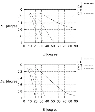
tfor eachElaveandElare shown in Fig. 4.
For same beam VLBI observation in which two nearby spacecraft are tracked simultaneously, RFP can be ex-pressed by traveling timetas:
2φ(t)=φ(t)−φ(t−t) . (32)
On the other hand, for switching VLBI observation in which two spacecraft are tracked alternately,RFP is calculated by differentiating the integrated RFP of two spacecraft as:
2φ(t)=
t=3Tsw
t=2Tsw
φ(t)dt+
t=Tsw
t=0
φ(t)dt 2
− t=2Tsw
t=Tsw
φ(t−t)dt , (33)
whereTswis the switching interval. In VRAD, the
switch-ing interval of one spacecraft includswitch-ing the slew time of 10 seconds is set to 60 seconds.
The RFP of the VLBI observation of the geosynchronous satellite (Liuet al., 2005) is used to evaluate the effect of tropospheric fluctuation onRFP. The weather was rainy in this observation. The effect of thermal noise can be
Transfer time of frozen block of water vapor [second]
58 26 9 7 3
0 10 20 30 40 50 60 70 80 90
Elave[degree]
0.1 0.2 0.3 0.4 0.5 0.6 0.7 0.8 0.9 1 El [degree]
Fig. 4. Transfer time of frozen block of water vaportfor average and difference of elevation angles of two spacecraft,ElandElave.
-60 -40 -20 0 20 40 60
0 1000 2000 3000 4000 5000
Residual fringe phase [degree]
Time [second]
Period.2
Fig. 5. Residual fringe phase of signal from geosynchronous satellite. “Period 2” represents observation period in which weather is rainy.
-25 -20 -15 -10 -5 0 5 10 15 20
0 1000 2000 3000 4000 5000
Differential Residual fringe phase [degree]
Time [second] t = 25 sec.
t = 9 sec. t = 1 sec.
Fig. 6. Differential residual fringe phase of S-band signal. Integration period is 50 seconds fortof 1, 9, and 25 seconds, respectively.
ignored because the C/N of the signal from the geosyn-chronous satellite is very large at 30 dB. Moreover, the ra-dio frequency of the signal from the geosynchronous satel-lite is 19.45 GHz, and the fluctuation of the ionospheric delay is very small in this frequency band. The RFP am-plitude is normalized by the ratio of the radio frequency of the geosynchronous satellite and Rstar/Vstar in the VRAD mission.
10-15 10-14 10-13 10-12
1 10 100
Allan standard deviation
Averaging time [second] RFP [Period.2] RFP, t = 1 second RFP, t = 9 seconds RFP, t = 25 seconds
Fig. 7. Allan standard deviations of residual fringe phase and differential residual fringe phase of S-band signal.
small. Figure 7 shows the ASD of RFP from Fig. 5 and RFP from Fig. 6. When averaging timeτ approachest, most tropospheric fluctuation is canceled out, and only the thermal noise, which is white noise, remains. Then ASD decreases at the rate of 1/τ whenτ is larger thant. On the other hand, both the tropospheric fluctuation and the thermal noise are superimposed whenτ is smaller thant. Since tropospheric fluctuation is considered a flicker noise, ASD slightly decreases in this range ofτ.
The phase error caused by the tropospheric fluctuations is evaluated from the RMS ofRFP. To satisfy the phase error condition in the MFV method, phase error must be smaller than 2.7 and 177.6 degrees in the S- and X-band sig-nals, respectively, by considering other error sources eval-uated in this section. For same beam VLBI observation in whichRFP is represented by Eq. (32), the phase error of S-band signal is 2.7 degrees in 50-second integration when t is 9 seconds. In this value oft, phase error of the X-band signal is 10 degrees. Therefore, the phase error condi-tion in the MFV method can be satisfied whentis smaller than 9 seconds.
On the other hand, for cases of switching VLBI obser-vation, the phase errors of the S- and X-band signals are calculated from Eq. (33). The shorter switching interval improves phase error of the differential phase delay in the case of the switching VLBI observation. By considering the slew time of the antenna and the integration period, about 20 second is the minimum value ofTswin the VRAD
mis-sion. Therefore, the phase errors are calculated for two cases:Tswis 20 and 60 seconds. Integration period is same
as switching interval. Figure 8 shows the phase errors of the S- and X-band signals. It is shown that the shorter switch-ing interval is effective to reduce the phase error. In ac-tual VLBI observation of the VRAD mission, an appropri-ate value of Tswwould be decided experimentally. On the
other hand, the phase error of the S-band signal does not become smaller than 2.7 degrees even ifTswis 20 seconds.
The phase error condition in the MFV method cannot be sat-isfied. This is because tropospheric fluctuations, whose pe-riods are shorter than the switching interval, still remain in theRFP. Consequently, under such rainy conditions as in this evaluation, the switching VLBI observation method is
17 18 19 20 21 22
0 10 20 30 40 50 60 70
Phase error of
RFP
(
) [degree]
t [second] S-band 2287 [MHz]
Tsw=50 seconds Tsw=20 seconds
60 65 70 75 80 85
0 10 20 30 40 50 60 70
Phase error of
RFP
(
) [degree]
t [second] X-band 8456 [MHz]
Tsw=50 seconds Tsw=20 seconds
Fig. 8. Phase errors of S- and X-band signals for cases of switching VLBI observation. Switching intervals are 20 and 60 seconds. Integration period is same as switching interval.
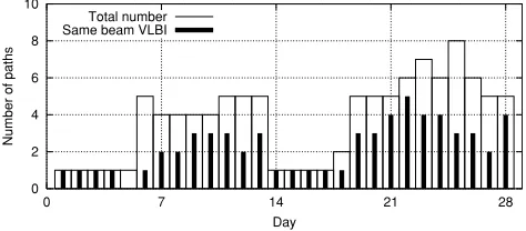
Table 4. Cut-off elevation angleElcut-offfor each VLBI observation mode of VRAD mission. Unit is degrees.
El Obs. type S-band/X-band Elcut-off
0.1 Same beam/Same beam 26
0.37 Same beam/Switching 58
insufficient, and the same beam VLBI observation method must be applied.
For same beam VLBI observation, the phase error condi-tion can be satisfied whent is smaller less than nine sec-onds. Therefore, cut-off elevation angle Elcut-off, in which
tis nine seconds, is estimated for each VLBI observation mode of the VRAD mission, as shown in Table 4. When Elave is larger than Elcut-off, the phase error condition can
be satisfied.
Also the phase error condition can be satisfied when the tropospheric fluctuation is larger than the data for this eval-uation. In this case,Elcut-offbecomes large compared to the
evaluated one in this section.
Finally, tropospheric fluctuation is modeled to embed it into the simulation model of the differential phase delay es-timation. Under the assumption of the Kolmogorov the-orem, the amplitudes of tropospheric fluctuations in time scales from 1 to 1000 seconds are nearly proportional to f43. The model of tropospheric fluctuationτtrop(t)is
repre-sented as:
τtrop(t)= 1
2πfrf
f=1
f=0.001
A· f−43sin
2πf ·t fsmp
+θ0(f)
,
(34) where frf is the radio frequency of the signal from the
10 20 30 40
50 60 70 80 90 El [degree] 0
0.20.4 0.60.8
1
El [degree] 0
0.05 0.1 0.15 0.2
Error of TEC [TECU]
Fig. 9. TEC error in differential residual fringe phase.
θ0(f)is the initial phase of each frequency component that
is provided in random order, and A is the amplitude of tropospheric fluctuation. A value for 0.005 during rainy days was used.
4.3 Ionospheric delay
The influence of the ionosphere was estimated in Liu et al.(2007) who showed that the TEC error condition in the MFV method is satisfied by the GPS method (Pinget al., 2002). However, the error of the differential phase delay depends on El and Elave. Moreover, when TID
occurs in the ionosphere (Afraimovich et al., 2000), the TEC condition in the MFV method is not satisfied even if the GPS method is applied. Therefore, the TEC errors included inRFP for each average and difference of the elevation angles of the two spacecraft are newly estimated by considering TID.
4.3.1 Average component of ionospheric delay The magnitude of average ionospheric delay is correlated with solar activity and the time of day. The estimated value of TEC above a GPS site near the VLBI station can be used for ionospheric calibration or global data can be used. Re-cently, the estimation error of TEC from GPS observation is about 2 TECU (Pinget al., 2002). The error of average ionospheric delayδτion is evaluated by mapping function
mion(El)(Otsuka et al., 2002) and the estimation error of
TECδTECzin the zenith angle:
δτion =√2·δTECz·m ion
El1
−mion
El2
. (35)
The typical altitude of ionosphere is set to 350 km. Figure 9 shows the TEC errors included inRFP for eachElaveand
El.
4.3.2 Dynamic component of ionospheric delay
TEC fluctuation can be characterized by TID (Afraimovich et al., 2000), which is classified by wavelength and ampli-tude as medium scale TID (MS-TID) and large scale TID (LS-TID). The typical amplitude and wavelength of TID areALS-TID=2 TECU andλLS-TID=1000 km for LS-TID
and AMS-TID = 1 TECU and λMS-TID = 300 km for
MS-TID (Afraimovichet al., 2000). The TEC estimation error caused by TID above the VLBI station is evaluated from its spatial distribution, which is shown in Fig. 10. Physi-cal separationx between the propagation paths from the ground station toward the two spacecraft is expressed as:
x= Hion·sin(El) sin(El1)·sin(El2)
. (36)
Fig. 10. Spatial distribution of TID above VLBI station.
1 0.6 0.3 0.1
0 10 20 30 40 50 60 70 80 90
El [degree] 0
0.2
0.4
0.6
0.8
1 El [degree]
1 0.6 0.3 0.1
0 10 20 30 40 50 60 70 80 90
El [degree] 0
0.2
0.4
0.6
0.8
1 El [degree]
Fig. 11. TEC error caused by MS-TID (Upper) and LS-TID (Lower). Unit is TECU.
In the case of VRAD,xis much smaller than the wave-length of MS-TID and LS-TID. The TEC difference be-tween the two propagation paths is approximately expressed as:
δTEC= √
2·2π·x·A
λ , (37)
whereAandλare the amplitude and the wavelength of MS-TID or LS-MS-TID. Figure 11 shows the TEC error for each ElaveandEl.
In the case of the switching VLBI observation of the two spacecraft, the TID transfer during switching interval Tsw
causes additional TEC error δTECsw. This TEC error is
expressed by replacingxin Eq. (37) byvTID·Tsw:
δTECsw=
√
2·2π·vTID·Tsw·A
λ , (38)
wherevTID is the velocity of the TID transfer. Assuming
thatvTIDis 0.1 km/s for MS-TID and 0.4 km/s for LS-TID
(Afraimovichet al., 2000), andTswis 60 seconds,δTECsw
Table 5. TEC error included in differential residual fringe phase of two nearby spacecraft. Difference of elevation angles between two spacecraft is 0.1 degrees. Unit is TECU.
A B C
Average Average Average
+MS-TID +LS-TID
Elave=17◦ 0.016 0.226 0.143
Consequently, the evaluation results of the TEC error are summarized. Table 5 shows the result for the same beam VLBI observation both in S- and X-bands. The TEC er-ror condition of 0.23 TECU can be satisfied when Elave
is larger than 17 degrees even if TID occurs in the iono-sphere above the VLBI station. Table 6 shows the result of same beam VLBI observation only in S-band and switching VLBI observation in X-band. The TEC error condition can also be satisfied when TID is absent. However, the TEC er-ror condition cannot be satisfied when TID occurs. Because X-band signals from two spacecraft are recorded alternately during this observation period, the change of TEC between switching intervals must be considered. “D” and “E” in Ta-ble 6 include the TEC error caused by the transfer of TID during switching intervals. Table 7 shows the result of the switching VLBI observation both in S- and X-bands. As in the case of Table 6, TEC error condition cannot be satis-fied when TID occurs. These evaluations show that in some cases, the TEC error condition cannot be satisfied due to the existence of TID.
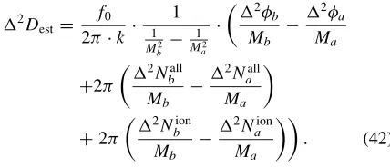
4.3.3 New TEC estimation method using multi-frequency signals To satisfy the conditions of the MFV method, a method for estimating the TEC error that still re-mains after differencing for the RFP of two spacecraft is newly proposed. RFP of the different frequency signals in VRAD can be used to estimate TEC error. As shown in Eq. (2), ionospheric delay is inversely proportional to the square of the radio frequency of the signal from the space-craft:
2τion = −k2D/f2
rf. (39)
Then TEC error2Dcan be estimated. TheRFP for the
signals of different frequenciesMa·f0andMb·f0from the
same crystal oscillator that generates reference frequency f0is expressed as:
2φ
where2τallis the sum of such non-dispersive delays as the geometric delay, the tropospheric delay, the instrumental delay, and the clock offset. 2Nall and 2Nion are the
cycle ambiguities of RFP that correspond to2τall and
2τion, respectively. Subscriptsaandbrepresent different
frequency signals. Ma and Mb are the coefficients of the frequencies of each signal. Radio frequency frfis expressed
as M · f0. For signalss2ands3 in VRAD (as described in
Section 2.2), Ma is 32, Mb is 33, and f0 is 69.3125 MHz
(Hanadaet al., 2002).
After eliminating2τallusing Eqs. (39), (40), and (41),
2Dis represented as:
est, two kinds of cycle ambiguity must be
corrected. Concerning the cycle ambiguity caused by TEC error,2Nion
a becomes equal to2Nbionwhen the following condition is satisfied: smaller than 0.83 TECU:
2D
This condition can only be satisfied when Elave is larger
than 20 degrees (El = 0.37 degrees) and 34 degrees
This condition can be satisfied using the differential group delay of signals s1, s2, and s3. As shown in Section 2.2
when TEC error and the phase error ofRFP are smaller than 810 TECU and 10.2 degrees, respectively, differential group delay can be derived within error of 2.8 ns without cycle ambiguity. TEC error of 810 TECU can be satisfied from the evaluation results of this section. When the phase error condition can be satisfied, Eq. (42) can be rewritten as the following equation:
The cycle ambiguity still remains in the 2nd term of Eq. (47). This term is 0.84 TECU, and there are some choices for2D
estevery 0.84 TECU. Then2Destcannot
be decided uniquely when2D
estis larger than 0.84 TECU.
When this condition is satisfied, 2D
estcan be estimated
Table 6. TEC error included in differential residual fringe phase of two nearby two spacecraft. Difference of elevation angles between two spacecraft is 0.37 degrees. Unit is TECU.
A B C D E
Average Average Average Average Average
+MS-TID +LS-TID +MS-TID +LS-TID
+transfer +transfer
Elave=20◦ 0.05 0.62 0.39 0.8 0.82
Table 7. TEC error included in differential residual fringe phase of two nearby spacecraft. Difference of elevation angles between two spacecraft is 0.9 degrees. Unit is TECU.
A B C D E
Average Average Average Average Average
+MS-TID +LS-TID +MS-TID +LS-TID
+transfer +transfer
Elave=34◦ 0.08 0.6 0.39 0.78 0.82
4.4 Position error of an a priori orbit
To estimate differential phase delay without cycle ambi-guity, the initial predicted geometric delay must be known with an accuracy of 83 ns (Konoet al., 2003). In the case of VRAD, where the shortest baseline is 1018 km (IRIKI-ISHIGAKI) (Kobayashi, 2005) and the distance between the spacecraft and ground station is 360,000 km, the error of the predicted orbits of two spacecraft must be less than 9.4 km. This accuracy can be achieved by orbit determi-nation with 2-way range and Doppler observations of the two spacecraft. The error, which is expected to be less than 7 km, corresponds to 61 ns. In the simulation model, the position error of an a priori orbit is included in the initial predicted geometric delay.
4.5 Other error sources
Other error sources in VLBI observations, which include clock offsetσclock, instrumental delayσinst, phase variation
in the main beam of receiving antenna σant-rx, and phase
variation caused by transmitting on-board antennaσant-txare
estimated in Liuet al.(2007). The results are summarized in Table 8. The magnitude of the phase error is common in the S- and X-band signals. As for the error of receiving antenna, it generates only when the same beam VLBI obser-vation is carried out because signals from the two spacecraft is not received at main beam center of antennas.
Largest parts of the instrumental delay can be canceled out by differencing the RFP of the signals from the two spacecraft. Therefore, the phase ripple generated at the VLBI front-end system is consideredσinst. In the
simula-tion, phase errorsσinst, σant-rx, andσant-tx are simply
con-sidered white noise. On the other hand, the clock offset is modeled as a linear function of the time.
4.6 Summary of error estimation
In this section, the error sources of differential phase delay are totally evaluated. The sources of the phase error of RFP are thermal noiseσS/N, tropospheric fluctuationσtrop,
σinst,σclock,σant-rx, andσant-tx. Among these terms,σclockand
σant-tx are almost zero, as described in Table 8. The total
phase error of RFP σφ is evaluated from the following equation:
σφ =
σ2
S/N+σinst2 +σant-rx2 +σtrop2 . (48)
Table 8. Phase error ofRFP of two spacecraft. Unit is all in degrees. σclock σinst σant-rx σant-tx
0 1 1.7 0
The total phase error in S- and X-band signalsσφs andσφx, is shown in Tables 9 and 10, respectively. In these tables, σS/Nandσtrop are the phase errors ofRFP, which are
in-tegrated over 50 seconds. Becauseσtropchanges with the
average and the difference of the elevation angle of the two VRAD spacecraft, cut-off elevation angleElcut-offfor
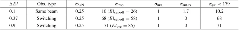
satis-fying the phase error condition is also shown in Tables 9 and 10. WhenElis smaller than 0.37 degrees, the phase error condition both in the S- and X-band signals can be satis-fied. The phase error condition in the S-band signal cannot be satisfied even if Elave is the maximum value of 85
de-grees in VRAD for the switching VLBI observation both in S- and X-bands. These results show that the condition of the phase error both in S- and X-bands can only be satisfied when the same beam VLBI observation method is applied.
TEC error2DinRFP must be less than 0.23 TECU,
as described in Section 2.2. From the evaluation result in Section 4.3.1, when TID does not occur in the ionosphere above the VLBI stations, the TEC error condition can be satisfied independent ofElaveandEl. On the other hand,
when TID does occur in the ionosphere, in some cases the TEC error condition cannot be satisfied. In this case, the new method to estimate2Dcan be used, as described in
Section 4.3.3. After compensating for TEC error with this method, the remaining TEC error is 0.04 TECU, and the condition of the TEC error can be satisfied.
The condition of the initial predicted geometric delay can also be satisfied as described in Section 4.4.
Next to the evaluation of the individual conditions of the MFV method, the four conditions described in Eqs. (20) to (23) are evaluated. To derive the differential phase delay of X-band signal without cycle ambiguity,σs2−s1, σs3−s1,σs1,
andσx1must be less than 0.5. Table 11 shows the evaluation
Table 9. Phase error ofRFP in S-band signal for different elevation angles of two spacecraft. Units are all in degrees.
El Obs. type σS/N σtrop σinst σant-rx σφs<4.3
0.1 Same beam 0.21 2.7 (Elcut-off=26) 1 1.7 3.4
0.37 Same beam 0.21 2.7 (Elcut-off=58) 1 1.7 3.4
0.9 Switching 0.21 19 (Elave=85) 1 0.0 19
Table 10. Phase error ofRFP in X-band signal for different elevation angles of two spacecraft.
El Obs. type σS/N σtrop σinst σant-rx σφx<179
0.1 Same beam 0.25 10 (Elcut-off=26) 1 1.7 10.2
0.37 Switching 0.25 68 (Elcut-off=58) 1 0 68
0.9 Switching 0.25 71 (Elave=85) 1 0 71
Table 11. Evaluation results of four conditions in MFV method in presence of TID.
Elongation Obs. type S-band/X-band Elcut-off σs2−s1 σs3−s1 σs1 σx1
El=0.1 Same beam/Same beam 26 [degrees] 0.38 0.17 0.44 0.13
El=0.37 Same beam/Switching 58 [degrees] 0.38 0.17 0.44 0.28
El=0.9 Switching/Switching 85 [degrees] 0.44 0.94 2.3 0.37
of the switching VLBI observation both in S- and X-bands, two of the four conditions cannot be satisfied. Although the σx1 condition is satisfied, all four conditions must be
satis-fied.
5.
Simulation Analysis of Differential Phase Delay
Estimation in VRAD
A simulation analysis of differential phase delay estima-tion is carried out using the models of the error sources un-der the predicted conditions of VRAD to assess the possible accuracy.
5.1 Description of simulation data
The signals from the spacecraft to the ground antennas are produced using the error sources modeled in Section 4. After the video conversion of the radio frequency signals, the signals received at the reference and remote stations are represented as:
xref(t)=Aref·exp{i(2π(frf− flocal)t
−2πfrf·τref(t)+θref)} +nthermalref (t) (49)
xrem(t)=Arem·exp{i(2π(frf− flocal)t
−2πfrf·τrem(t)+θrem)} +nthermalrem (t) ,(50)
where
τi(t)=τigeo(t)+τiinst(t)+τiclock(t)+τ
trop
i (t) +τion
i (t) (i=ref,rem), (51)
where subscriptirepresents the reference station as ref and the remote station as rem. Timetis epoch when the signal is received at the reference station, frfis the radio frequency
of the signals, flocal is the frequency of the local signals,
andArefandAremare the amplitudes of the signals for each
station, respectively. Phaseθirepresents the sum of the ini-tial phase for the local signal of the video converter and the phase of the signal when it is transmitted from the space-craft. This is given as a constant value. Propagation time
from the spacecraft to ground stationτi(t)is the sum of geo-metric propagation timeτigeo(t), tropospheric delayτitrop(t), ionospheric delay τion
i (t), instrumental delay τiinst(t), and the clock offset between ground stations τclock
i (t). As de-scribed in Eq. (29), the thermal noise of the ground system is given bynthermali (t).
The simulation orbits of two spacecraft are produced us-ing the GEODYN II program (Pavliset al., 2001). The or-bital elements are shown in Table 2. Lunar gravity field model LP100J (Konoplivet al., 2001) is used in this simu-lation.
Tropospheric delayτitrop(t)is composed of the average component and its fluctuation. Average tropospheric delay is given as a product of the error of the zenith wet delay and the mapping function, as described in Section 4.2.1. The error of the zenith wet delay is assumed to be 17 ps (Eloseguiet al., 1998). Tropospheric fluctuation in Eq. (34) is added to the signal from Rstar and Vstar by shifting the time with the amount oftin Eq. (31), wheretdepends on the average and the difference of the elevation angles of Rstar and Vstar.
Ionospheric delayτiion(t)is only the average component because its fluctuation caused by TID can be corrected for by the new method that estimates TEC error, as described in Section 4.3.3. Average ionospheric delay is given as a product of the error of the zenith ionospheric delay and the mapping function, as described in Section 4.3.1, which is identical for the tropospheric delay. TEC error in the zenith angle is assumed to be 2 TECU (Pinget al., 2002).
5.2 Conditions for simulation analysis of same beam VLBI observation
0 0.1 0.2 0.3 0.4 0.5 0.6 0.7 0.8 0.9
11:30:00 12:00:00 12:30:00 13:00:00 13:30:00
Elongation [deg.]
August 10, 2003 [UT]
MIZUSAWA OGASAWARA ISHIGAKI IRIKI
45 50 55 60 65 70 75
11:30:00 12:00:00 12:30:00 13:00:00 13:30:00
Average elevation angle [deg.]
August 10, 2003 [UT] MIZUSAWA
OGASAWARA ISHIGAKI IRIKI
Fig. 12. Average elevation angle and elongation of Rstar and Vstar in simulation path on August 10, 2003.
Table 12. Types of VLBI observation in each period. Period Obs. type S-band/X-band 11:30:00–12:03:00 Switching/Switching 12:03:00–12:28:00 Same beam/Switching 12:28:00–13:30:00 Same beam/Same beam
Figure 13 shows the residual geometric delay (RGD) of Rstar and Vstar. In this simulation differential RGD, which is the difference between the RGD of Rstar and Vstar, will be estimated as a differential phase delay.
5.3 Same beam VLBI observation both in S- and X-bands
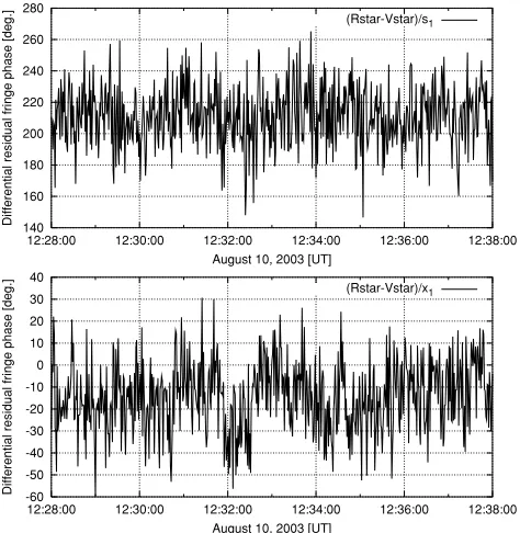
5.3.1 Correlation results The simulation signals represented in Eqs. (49) and (50) are correlated by the soft-ware method (Konoet al., 2003; Kikuchiet al., 2004). Fig-ure 14 shows the RFP of the signals from Rstar and Vstar for the MIZUSAWA–OGASAWARA baseline (Kobayashi, 2005). The integration period is one second. One of the three S-band signals1 whose frequency is 2212 MHz and
one X-band signalx1are shown. The change with the time
of RFP caused by the residual geometric delay is removed to show the RFP variation caused by tropospheric fluctua-tion.
Figure 15 shows theRFP between the signals of Rstar and Vstar. The tropospheric fluctuation of RFP whose pe-riod is longer thantof 2 seconds is almost canceled out. The RMS of RFP is 12.8 degrees in S-band and 41.4 de-grees in X-band. The RMS ofRFP is reduced to 2.2 and 8.1 degrees as a result of RFP differentiation. Integration time is set to 50 seconds.
The RMS ofRFP is almost consistent with the phase errors modeled in the simulation. That is, the phase error of the S-band signal, σS/N, σinst, and σant-rx are assumed
-60 -40 -20 0 20 40 60
11:40:00 12:00:00 12:20:00 12:40:00 13:00:00 13:20:00
Residual geometric delay [ns]
August 10, 2003 [UT]
Rstar Vstar Rstar - Vstar
Fig. 13. Residual geometric delay of Rstar and Vstar and differential residual geometric delay of these residual geometric delays.
to be 0.21, 1, and 1.7 degrees, respectively, as shown in Table 9. The phase error of tropospheric fluctuationσtrop
is 0.6 degrees when it is calculated using Eqs. (32) and (34) when thet condition is 2 seconds. Therefore, the phase error of RFP calculated from Eq. (48) becomes 2.3 degrees and is almost identical to the RMS ofRFP. The small difference is caused by the change with time of t in the simulation. Consequently, this result confirms the availability of the simulation model. Additionally, the ASDs of RFP and RFP shown in Fig. 16 represent the characteristics of the actual tropospheric fluctuations well compared with the ASDs in Fig. 7.
5.3.2 Results for differential phase delay estimation
At first, the estimation of the difference of cycle ambiguity Ns2−Ns1 between signalss1ands2, whose frequency
interval is 6 MHz, was carried out using Eq. (16). To uniquely estimateNs2−Ns1, the conditions ofNs2−
Ns1in Table 1 and Eq. (20) must be satisfied. The absolute
value of differential residual geometric delay is smaller than 20 ns in this simulation period. TEC error included in RFP is smaller than 0.01 TECU, as seen in Fig. 9. That is,Elaveis about 52 degrees andEl is about 0.1 degrees
in the simulation period. The phase error forRFP of the S-band signals is 15.6 degrees in one-second integration.
From Eq. (20), σs2−s1 becomes 0.18, and the condition
for the estimation ofNs2−Ns1is satisfied. As shown in
Fig. 17,Ns2−Ns1can be derived uniquely.
Second, the estimation of the difference of cycle ambi-guityNs3−Ns1 between signalss1ands3, whose
fre-quency interval is 75 MHz, is conducted using Eq. (17). To uniquely estimateNs3−Ns1, its conditions in Table 1
and Eq. (21) must be satisfied. The phase error condition can be satisfied by integratingRFP. The phase error is 4 degrees for 15-second integration. TEC error is identical as the estimation ofNs2−Ns1.
From Eq. (21),σs3−s1becomes 0.2, and the condition for
the estimation of cycle ambiguityNs3−Ns1is satisfied.
Figure 18 shows the error ofNs3 −Ns1 in which the
integration period ofRFP is 1 and 15 seconds. Although Ns3 −Ns1 is not decided uniquely for the 1-second
integration, it converges to 0 in the 15-second integration. Third, the estimation of cycle ambiguityNs1 of signal
s1, whose frequency is 2212 MHz, is carried out using
Eq. (18). To uniquely estimate Ns1, its conditions in
-30 -20 -10 0 10 20 30 40 50 60 70 80
12:28:00 12:30:00 12:32:00 12:34:00 12:36:00 12:38:00
Residual fringe phase [deg.]
August 10, 2003 [UT] Rstar/s1
-240 -220 -200 -180 -160 -140 -120
12:28:00 12:30:00 12:32:00 12:34:00 12:36:00 12:38:00
Residual fringe phase [deg.]
August 10, 2003 [UT] Vstar/s1
-100 -50 0 50 100 150
12:28:00 12:30:00 12:32:00 12:34:00 12:36:00 12:38:00
Residual fringe phase [deg.]
August 10, 2003 [UT] Rstar/x1
-50 0 50 100 150 200
12:28:00 12:30:00 12:32:00 12:34:00 12:36:00 12:38:00
Residual fringe phase [deg.]
August 10, 2003 [UT] Vstar/x1
Fig. 14. Residual fringe phases of carrier wave signals from Rstar and Vstar in one-second integration periodss1represent the S-band signal whose frequency is 2212 MHz andx1represents one X-band signal.
140 160 180 200 220 240 260 280
12:28:00 12:30:00 12:32:00 12:34:00 12:36:00 12:38:00
Differential residual fringe phase [deg.]
August 10, 2003 [UT]
(Rstar-Vstar)/s1
-60 -50 -40 -30 -20 -10 0 10 20 30 40
12:28:00 12:30:00 12:32:00 12:34:00 12:36:00 12:38:00
Differential residual fringe phase [deg.]
August 10, 2003 [UT]
(Rstar-Vstar)/x1
Fig. 15. Differential residual fringe phases of carrier wave signals between Rstar and Vstar in one-second integration periods. s1represents the S-band signal whose frequency is 2212 MHz and x1 represents one X-band signal.
ofRFP becomes 2.2 degrees for a 50-second integration period. TEC error is identical to the estimation ofNs2−
Ns1.
From Eq. (22),σs1 becomes 0.27. The condition for the
estimation of cycle ambiguityNs1 is satisfied, andNs1
can be derived uniquely. Figure 19 shows the estimated differential phase delay of signal s1 in the 50-second
in-tegration period. The offset and RMS are 2.7 and 5.5 ps.
10-14 10-13 10-12 10-11
1 10 100
Allan standard deviation
Averaging time [second] RFP RFP
Fig. 16. Allan standard deviations of residual fringe phase and differential residual fringe phase of S-band signals1.
The offset value comes from the TEC error of 0.01 TECU and the RMS value comes from the phase error ofRFP of 2.2 degrees.
Finally, the estimation of cycle ambiguityNx1of signal
x1, whose frequency is 8456 MHz, is carried out using
Eq. (19). To uniquely estimate Nx1, its conditions in
Table 1 and Eq. (23) must be satisfied. For the X-band signal, phase error is 8.1 degrees for a 50-second integration period. TEC error is identical to the estimation ofNs2−
Ns1.
From Eq. (23),σx1 becomes 0.05. The condition for the
estimation of cycle ambiguityNx1is satisfied. Figure 20
shows the estimated differential phase delay of signalx1in
the 50-second integration period. The offset and RMS of the estimated differential phase delay are 0.2 ps and 2.9 ps, respectively.
Consequently, the desired accuracy of the differential phase delay of signal x1 in the VRAD mission can be
-1 -0.5 0 0.5 1
12:30:00 12:40:00 12:50:00 13:00:00 13:10:00 13:20:00
Error of cycle ambiguity
August 10, 2003 [UT] Integration period = 1 sec.
Ns
2-Ns1
Fig. 17. Error of derived cycle ambiguityNs2−Ns1between signals
s1ands2. The integration period of the differential residual fringe phase is one second.
-5 -4 -3 -2 -1 0 1 2 3 4
12:30:00 12:40:00 12:50:00 13:00:00 13:10:00 13:20:00
Error of cycle ambiguity
August 10, 2003 [UT] Integration period = 1 sec.
Ns
3-Ns1
-1 -0.5 0 0.5 1
12:30:00 12:40:00 12:50:00 13:00:00 13:10:00 13:20:00
Error of cycle ambiguity
August 10, 2003 [UT] Integration period = 15 sec.
Ns
3-Ns1
Fig. 18. Error of derived cycle ambiguityNs3−Ns1between signals
s1 ands3. Integration period of differential residual fringe phase is 1 and 15 seconds, respectively.
5.4 Same beam VLBI observation in S-band only and switching VLBI observation in X-band
5.4.1 Connecting RFP of X-band signal without cy-cle ambiguity For same beam VLBI observation in S-band only and switching VLBI observation in X-S-band, the RFP of the X-band signals from two spacecraft are ob-tained alternately. This section describes how to calculate theRFP of X-band signals. A polynomial fitting method is used because changes of RFP mainly depend on the er-ror of the spacecraft’s a priori orbit. For example, the case shown in Fig. 21 is considered. To calculateRFP in Pe-riod 2, first the polynomial function is calculated from the RFP of spacecraft A in Periods 1 and 3. Then the RFP of spacecraft B in Period 2 is integrated at the central epoch of Period 2. After that,RFP is calculated from the difference between the integrated RFP of spacecraft B in Period 2 and the RFP of spacecraft A in the central epoch of Period 2, which is interpolated from the polynomial function.
-10 -5 0 5 10
12:30:00 12:40:00 12:50:00 13:00:00 13:10:00 13:20:00 13:30:00
Error of differential phase delay [ps]
August 10, 2003 [UT] 50 second integration
Ns1
Fig. 19. Error of estimated differential phase delay of signals1 in a 50-second integration period.
-10 -5 0 5 10
12:30:00 12:40:00 12:50:00 13:00:00 13:10:00 13:20:00 13:30:00
Error of differential phase delay [ps]
August 10, 2003 [UT] 50 second integration
Nx1
Fig. 20. Error of estimated differential phase delay of signalx1in 50-sec-ond integration period.
Fig. 21. Connecting RFP of X-band signal without cycle ambiguity.
Note that the cycle ambiguity of RFP between the switch-ing interval must be compensated for before calculatswitch-ing RFP. The change with time of RFP caused by the dis-persive and non-disdis-persive delays must be considered sep-arately. As for the dispersive ionospheric delay, when the difference of TEC D(t)changes 3.2 TECU during the switching interval, the RFP change exceeds 180 degrees, as seen in Eq. (3) , which generates cycle ambiguity. However, D(t) can be compensated for within error of 2 TECU (Ping et al., 2002). As for the non-dispersive delays, the tropospheric fluctuation rarely exceeds 180 degrees during the switching interval of 60 seconds because the ASD of the RFP is smaller than 5×10⁻¹³even if the climate condition
com-Table 13. Conditions for estimating cycle ambiguitiesNs2−Ns1,Ns3−Ns1,Ns1, andNx1.
σ
φs 2D 2τs σφx
Ns2−Ns1 3.8 [degrees] 0.01 [TECU] 48 [ns] — σNs2−Ns1=0.3 Ns3−Ns1 3.8 [degrees] 0.01 [TECU] — — σNs3−Ns1=0.19
Ns1 3.8 [degrees] 0.01 [TECU] — — σNs1=0.45
Nx1 3.8 [degrees] 0.01 [TECU] — 68 [degrees] σNx1 =0.22
-60 -50 -40 -30 -20 -10 0 10 20 30 40
12:00:00 12:05:00 12:10:00 12:15:00 12:20:00 12:25:00 12:30:00
Error of differential phase delay [ps]
August 10, 2003 [UT] 50 second integration
Nx1
Fig. 22. Error of differential phase delay of signalx1. Integration period of differential residual fringe phase is 50 seconds.
pensated by the polynomial fitting method. Consequently, the RFP of the X-band signal can be estimated without cy-cle ambiguity during the switching interval.
5.4.2 Results for differential phase delay estimation
From RFP calculated by the method described in Sec-tion 5.4.1, differential phase delay estimaSec-tion is carried out. The conditions for deriving the cycle ambiguity for each frequency band are summarized in Table 13. The error sources are somewhat large compared with those in the case of the same beam VLBI observation both in the S- and X-bands described in Section 5.3.2. These differences are mainly caused by elongation of the two spacecraft. How-ever, all the conditions for deriving the cycle ambiguity of each frequency band are satisfied.
Figure 22 shows the error of the differential phase delay of the X-band signal estimated by the MFV method. The RMS error of the differential phase delay in a 50-second in-tegration period is 22.5 ps. In this simulation period, the phase error of RFP caused by the tropospheric fluctuations whose periods are shorter than the switching interval cannot be removed for the X-band signal. Therefore, the error of the differential phase delay of the X-band signal is some-what large compared to Fig. 20.
5.5 Switching VLBI observation in both S- and X-bands
When the climate condition is rainy, as discussed in Sec-tion 4.2.2 and/or TID occurs in the ionosphere above the VLBI station, as discussed in Section 4.3.2, satisfying the conditions of differential phase delay estimation by MFV method is impossible. However, the period of switching VLBI observation accounts for most of the observation pe-riod in the VRAD mission. Therefore, the differential phase delay of the X-band signal must be obtained in the period of switching VLBI observation. Fortunately, there are paths in which same beam VLBI observation can be carried out for at least 50 seconds, including more than 90% of the total
Fig. 23. Method to estimate differential phase delay during period of switching VLBI observation.
-60 -40 -20 0 20 40 60 80
11:30:00 11:35:00 11:40:00 11:45:00 11:50:00 11:55:00 12:00:00 12:05:00
Error of differential phase delay [ps]
August 10, 2003 [UT] 50 second integration
Nx1
Fig. 24. Error of differential phase delay of signalx1. Integration period of differential residual fringe phase is 50 seconds.
paths described in Section 3.2. Path here denotes the con-tinuous observation period of the spacecraft. A method to derive differential phase delay without cycle ambiguity in these paths is newly developed.
For example, for the continuous observation path shown in Fig. 23, assume that same beam VLBI observation is car-ried out in period “A” in Fig. 23, and switching VLBI ob-servation is carried out in period “B”. The results in Sec-tions 5.3 and 5.4 show that the cycle ambiguity ofRFP of the X-band signal can be derived by applying the same beam VLBI observation method. Therefore, the derived cle ambiguity in Period “A” can be applied to derive the cy-cle ambiguity in Period “B”. The differential phase delay of the X-band signal in Period “B” is represented as follows:
2τB x1(t)=
2φB x1(t)
2πfrf
+2π·NxA1
2πfrf
, (52)
where2φB(t)is theRFP of the X-band signal in Period “B” andNA
x1 is the cycle ambiguity of RFP of the