Mean square numerical solution of stochastic differential equations by fourth order Runge Kutta method and its application in the electric circuits with noise

(1)

R E S E A R C H

Open Access

Mean square numerical solution of stochastic

differential equations by fourth order

Runge-Kutta method and its application in

the electric circuits with noise

Morteza Khodabin

1*

_{and Majid Rostami}

2

*_{Correspondence:}

[email protected]

1_{Department of Mathematics,}

College of Basic Sciences, Karaj Branch, Islamic Azad University, Alborz, Iran

Full list of author information is available at the end of the article

Abstract

We consider numerical solutions of stochastic initial value problems via the random Runge-Kutta method of the fourth order. A random mean value theorem is

established and the mean square convergence of these methods is proved. The expectation and variance of the solution are derived. We supplement this method by plotting computational errors.

Keywords: stochastic diﬀerential equation; random fourth order Runge-Kutta method; random mean value theorem; mean square solution

1 Introduction

Stochastic differential equations (SDEs) have many applications in economics, ecology, and finance [–]. In recent years, the development of numerical methods for the approx-imation of SDEs has become a field of increasing interest; seee.g.[–] and references therein. For example in [], a numerical solution of SDEs is given by a random Euler method and in [–], we obtain the expectation and variance of a numerical solution of these equations by a random Runge-Kutta method of the second order that have good ac-curacy, with respect to the Euler method [], and in this paper we obtain the expectation and variance of numerical solution of these equations by a random Runge-Kutta method of the fourth order.

A stochastic diﬀerential equation of the form

˙

X(t) =f(X(t),t), t∈I= [t,T],

X(t) =X, ()

where X is a random variable, and the unknown X(t) as well as the right-hand side

f(X(t),t) are stochastic processes deﬁned on the same probability space (,,P), are pow-erful tools to model real problems with uncertainty. The authors of [] treated the nu-merical solution of stochastic initial value problems based on a sample treatment of the right-hand side of the diﬀerential equations. The sample treatment approach developed in [] has the advantage that conclusions remain true in the deterministic case, but in

(2)

many situations the hypotheses assumed in [] are not satisﬁed. This fact motivates re-search for alternative conditions under which good numerical approximations could be constructed. Here we do not assume any trajectorial condition but mean square change information off(X(t),t) is expressed in terms of its mean square modulus of continuity. Other numerical schemes for stochastic diﬀerential equations may be found in [, , , ].

This paper is organized as follows: Section  deals with some preliminaries addressed to clarify the presentation of concepts and results used later. A mean value theorem for stochastic processes is given in Section  and in Section  the mean square convergence of a random fourth order Runge-Kutta method is established. In Section  some examples of [, ] illustrate the accuracy of the presented results. Finally, Section  gives some brief conclusions.

2 Preliminaries

Deﬁnition  We are interested in second order random variablesX, having a density func-tionfX,

EX= ∞

–∞x

_f

X(x)dx<∞,

whereEdenotes the expectation operator, and it allows the introduction of the Banach spaceLof all the second order random variables endowed with the norm

X=

EX_.

Deﬁnition  A stochastic processX(t) deﬁned on the same probability space (,,P) is called a second order stochastic process if for eacht,X(t) is a second order random variable. Hence the meaning ofX˙(t) in () is the mean square limit inLof the expression

X(t+t) –X(t)

t , ast→.

Lemma  Let Xnand Ynbe two sequences of second order random variables mean square convergent to the second order random variable X,Y,respectively,i.e.,

Xn→X and Yn→Y as n→ ∞,

then

E[XnYn]→E[XY] as n→ ∞,

and so

lim

n→∞E[Xn] =E[X] and nlim→∞Var[Xn] =Var[X].

Deﬁnition  Letg:I−→Lbe a mean square bounded function and leth> , then the

mean square modulus of continuity ofgis the function

ω(g,h) = sup

|t–t∗|≤h

(3)

Deﬁnition  The functiongis said to be mean square uniformly continuous inI, if

lim

h→ω(g,h) = .

Deﬁnition  Letf(X,t) be deﬁned onS×IwhereSis a bounded set inL. We say thatf

is randomly bounded uniformly continuous inS, if

lim

h→ω

f(X,·),h = ,

uniformly forX∈S, and ﬁnally we have

sup

X∈S

ωf(X,·),h =ω(h)→.

Deﬁnition  Let{Nt}t≥be an increasing family ofσ-algebras of sub-sets of. A process g(t,ω) from [,∞)×toRn_{is called}_Nt_{-adapted if for each}_t_≥_{ the function}_ω_→_g₍_t_,_ω₎

isNt-measurable, [].

Deﬁnition  Letν=ν(S,T) be the class of functionsf(t,ω) : [,∞)×→Rsuch that: (i) (t,ω)→f(t,ω)isB×F-measurable, whereBdenotes the Borelσ-algebra on

[,∞)andFis theσ-algebra on,

(ii) f(t,ω)isFt-adapted, whereFtis theσ-algebra generated by the random variables Bs;s≤t,

(iii) E[_STf₍_t_,_ω₎_dt_{] <}_∞_{, [].}

Deﬁnition (The Itô integral), [] Letf ∈ν(S,T), then the Itô integral off (fromSto

T) is deﬁned by

T

S

f(t,ω)dBt(ω) = lim

n→∞

T

S

φn(t,ω)dBt(ω),

whereφnis a sequence of elementary functions such that

E

T

S

f(t,ω) –φn(t,ω) dt

→, asn→ ∞.

Theorem (The Itô isometry), [] Let f ∈ν(S,T),then

E

T

S

f(t,ω)dBt(ω) 

=E

T

S

f(t,ω)dt

.

Deﬁnition (-dimensional Itô processes), [] LetBt be -dimensional Brownian

mo-tion on (,F,P). A (-dimensional) Itô process (or stochastic integral) is a stochastic pro-cessXton (,F,P) of the form

Xt=X+ t



u(s,ω)ds+ t



(4)

where

P

t



v(s,ω)ds<∞, for allt≥

= ,

P

t



u(s,ω)ds<∞, for allt≥

= .

The Itô processesXtis sometimes written in the shorter diﬀerential form

dXt=u dt+v dBt. ()

Theorem (The -dimensional Itô formula), [] Let Xtbe an Itô process given by()and g(t,x)∈C_([,_∞₎_×_R_),_then

Yt=g(t,Xt)

is again an Itô process,and

dYt=∂g

∂t(t,Xt)dt+ ∂g

∂x(t,Xt)dXt+

 

∂_g

∂x(t,Xt)(dXt)

_, _()

where(dXt)_{= (}_dXt₎₍_dXt₎_{is computed according to the rules}

dt·dt=dt·dBt=dBt·dt= , dBt·dBt=dt. ()

Lemma [] Let X(t)be a second order stochastic process,mean square continuous on I= [t,T],then there existsη∈I such that

t

t

X(s)ds=X(η)(t–t), t<t<T.

The purpose of the theorem below is to establish a relationship between the increment

X(t) –X(t) of a second order stochastic process, and its mean square derivativeX˙(η) for someηin [t,t] fort>t. The result will be used to prove the convergence of the random Runge-Kutta method.

Theorem  Let X(t)be a mean square diﬀerentiable second order stochastic process in

I= [t,T]and mean square continuous in it.Then there existsη∈I such that

X(t) –X(t) =X˙(η)(t–t).

Proof See [].

3 Convergence of random fourth order Runge-Kutta method A random fourth order Runge-Kutta method will have the following form:

Xn+=Xn+

(5)

where ⎧ ⎪ ⎪ ⎪ ⎨ ⎪ ⎪ ⎪ ⎩

k=hf(Xn,tn), k=hf(Xn+k

,tn+ h ), k=hf(Xn+k

,tn+ h ), k=hf(Xn+k,tn+h).

()

Theorem  Let f(X(t),t)be deﬁned on S×I to L,where S is a bounded set in L.If f(X(t),t) satisﬁes the conditions(C)and(C),

(C) f(X,t)is randomly bounded uniformly continuous,

(C) f(X,t)satisﬁes the mean square Lipschitz condition,that is,

f(X,t) –f(Y,t)≤k(t)X–Y, ()

where_tT

k(t)dt<∞,

then the random fourth order Runge-Kutta scheme()is mean square convergent.

Proof Note that under hypotheses (C) and (C), we are interested in the mean square convergence to zero of the error

en=Xn–X(tn), ()

whereX(t) is the theoretical solution of the fourth order stochastic process of the prob-lem ().

From Theorem  it follows that

X(tn+) =X(tn) +hfX(tη),tη , tη∈(tn,tn+). ()

By (), (), (), and () it follows that

en+ ≤ en+h

f(Xn,tn) –f

X(tη),tη +

h

 f

Xn+ k

,tn+

h



–fX(tη),tη

+h  f

Xn+k ,tn+

h



–fX(tη),tη

+h

f(Xn+k,tn+h) –f

X(tη),tη . ()

By assumption

M= sup

t≤t≤T

X˙(t), ()

and using (C), (C), and Theorem  we have

f(Xn,tn) –f

X(tη),tη ≤f(Xn,tn) –f

X(tn),tn +f

X(tn),tn –f

X(tη),tn

+fX(tη),tn –fX(tη),tη

(6)

and

and by setting

an=  + h

the inequality () gets the following form:

en+ ≤anen+bn, n= , , , . . . , ()

and by successive substitution, () will become

en+ ≤

and by () and geometrical progression we conclude

(7)

Finally, from () and substituting () and () in (), we obtain the following error bound:

en+ ≤ exp

(n+ )h



k(tn) + k

tn+h 

+k(tn+h)

e

+exp((n+ )

h

[k(tn) + k(tn+ h

) +k(tn+h)]) –  h

[k(tn) + k(tn+ h

) +k(tn+h)]

×

Mh 

k(tn) +Mh

_k

tn+h 

+Mh



 k(tn+h) +hω(h)

; ()

by assumptione=  andnh=T–t, the above inequality can be written as

en+ ≤ exp( T–t+h

 [k(T) + k(T+ h

) +k(T+h)]) –  k(T) + k(T+h_) +k(T+h)

×

Mhk(T) + Mhk

T+h 

+ Mhk(T+h) + ω(h)

; ()

sinceω(h)→ ash→, by condition (C) and inequality () we can deduce that the sequenceenis mean square convergent to zero ash→. Thus we have established the

theorem.

4 Numerical examples

Here we present some examples. Since these examples can be found in [, ], we can com-pare the results.

Example  Consider the following problem:

˙

X(t) = tX(t) +exp(–t) +B(t), t∈[, ],

X() =X,

()

where B(t) is a Brownian motion process and X is a normal random variable, X∼ N(_,_) independent ofB(t) for eacht∈[, ].

For computing the exact solution of the problem, by multiplying the equation by exp(–t_{) and using}_W₍_t_{) =}dB(t)

dt , we have

–texp–t X(t)dt+exp–t dX(t) =exp–t exp(–t) +B(t) dt

using the Itô formula [], we deduce

dexp–t X(t) = –texp–t X(t)dt+exp–t dX(t) =exp–t exp(–t) +B(t) dt

and so

X(t) =expt X+

t



exp–s exp(–s) +B(s) ds

(8)

Iff(X(t),t) = tX(t) +exp(–t) +B(t), we have

f(X,t) –fX,t∗ ≤X+  t–t∗+t–t∗ _()

sof(X,t) is randomly bounded uniformly continuous in any bounded setS⊂L. Now, from the random fourth order Runge-Kutta method we have

Xn+=Xn+

and by setting

(9)

(10)

Table 1 Absolute error of the expectation ofX(t) with the Euler, RK2, and RK4 methods and h=₂₀1,h=₅₀1

t Euler RK2 RK4

h =₂₀1 h =₅₀1 h =₂₀1 h =₅₀1 h =₂₀1 h =₅₀1

t Euler RK2 RK4

h =₂₀1 h =₅₀1 h =₂₀1 h =₅₀1 h =₂₀1 h =₅₀1

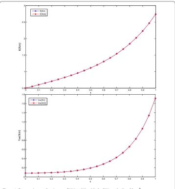
The absolute error of the expectation and variance ofX(t) with the Euler, RK and RK methods and h=_, h=_ are shown in Tables , . In Figure , the expectation and variance of the exact and numerical solutions of Example  with the RK method and

(11)

Figure 1 Expectations and variances ofX(t) andXnwith the RK4 method andh=201.

Example  Consider the following initial value problem:

˙

X(t) =t_X₍_t_{) +}_W₍_t_), _t_∈_{[, ],}

X() =X, ()

whereW(t) is a Gaussian white noise process with mean zero andXis an exponential

ran-dom variable with parameterλ=_, independent ofW(t) for eacht∈[, ]. Heref(X(t),t) involves the white noise process with mean zeroW(t),i.e. f(X(t),t) =t_X₍_t_{) +}_W₍_t_).

The covariance ofW(t) is

CovW(t),W(s)=δ(t–s), ()

(12)

for multiplication,

δ∗g=g.

So, takingg(s) =h(s)χ[,t](s), whereh(s) is aC∞function andχ[,t](s) denotes the

charac-teristic function on the interval [,t], from () it follows that ∞

For computing the exact solution of the problem, by multiplying both sides of () by exp(–t_), and usingW(t) =dB(t)_dt , we have

using the Itô formula, [], we conclude

d

Now, we computeXnfrom the random fourth order Runge-Kutta method,

Xn+=Xn+

and by setting

(13)

(14)

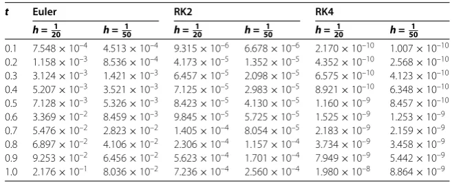
Table 3 Absolute error of the expectation ofX(t) with the Euler, RK2 and RK4 methods and h=₂₀1,h=₅₀1

t Euler RK2 RK4

h =₂₀1 h =₅₀1 h =₂₀1 h =₅₀1 h =₂₀1 h =₅₀1

0.1 7.548×10–4 _4.513_×₁₀–4 _9.315_×₁₀–6 _6.678_×₁₀–6 _2.170_×₁₀–10 _1.007_×₁₀–10 0.2 1.158×10–3 _8.536_×₁₀–4 _4.173_×₁₀–5 _1.352_×₁₀–5 _4.352_×₁₀–10 _2.568_×₁₀–10 0.3 3.124×10–3 _1.421_×₁₀–3 _6.457_×₁₀–5 _2.098_×₁₀–5 _6.575_×₁₀–10 _4.123_×₁₀–10 0.4 5.207×10–3 _3.521_×₁₀–3 _7.125_×₁₀–5 _2.983_×₁₀–5 _8.921_×₁₀–10 _6.348_×₁₀–10 0.5 7.128×10–3 _5.326_×₁₀–3 _8.423_×₁₀–5 _4.130_×₁₀–5 _1.160_×₁₀–9 _8.457_×₁₀–10 0.6 3.369×10–2 _8.459_×₁₀–3 _9.845_×₁₀–5 _5.725_×₁₀–5 _1.525_×₁₀–9 _1.253_×₁₀–9 0.7 5.476×10–2 _2.823_×₁₀–2 _1.405_×₁₀–4 _8.054_×₁₀–5 _2.183_×₁₀–9 _2.159_×₁₀–9 0.8 6.897×10–2 4.106×10–2 2.306×10–4 1.157×10–4 3.734×10–9 3.458×10–9 0.9 9.253×10–2 6.456×10–2 5.623×10–4 1.701×10–4 7.949×10–9 5.442×10–9 1.0 2.176×10–1 8.036×10–2 7.236×10–4 2.560×10–4 1.980×10–8 8.864×10–9

Table 4 Absolute error of variance ofX(t) with the Euler, RK2, and RK4 methods andh=₂₀1, h=₅₀1

t Euler RK2 RK4

h =₂₀1 h =₅₀1 h =₂₀1 h =₅₀1 h =₂₀1 h =₅₀1

0.1 5.425×10–1 _4.215_×₁₀–1 _9.914_×₁₀–2 _9.807_×₁₀–2 _9.74098_×₁₀–2 _6.206_×₁₀–2 0.2 6.456×10–1 _5.452_×₁₀–1 _2.243_×₁₀–1 _1.968_×₁₀–1 _1.95502_×₁₀–1 _8.245_×₁₀–2 0.3 8.425×10–1 _6.152_×₁₀–1 _3.654_×₁₀–1 _2.980_×₁₀–1 _2.96196_×₁₀–1 _1.312_×₁₀–1 0.4 8.896×10–1 _7.431_×₁₀–1 _5.756_×₁₀–1 _4.049_×₁₀–1 _4.02421_×₁₀–1 _2.318_×₁₀–1 0.5 9.476×10–1 _8.189_×₁₀–1 _7.265_×₁₀–1 _5.219_×₁₀–1 _5.18782_×₁₀–1 _3.436_×₁₀–1 0.6 3.523×10–0 _1.078_×₁₀–0 _8.438_×₁₀–1 _6.558_×₁₀–1 _6.51931_×₁₀–1 _4.540_×₁₀–1 0.7 4.247×10–0 _3.368_×₁₀–0 _9.457_×₁₀–1 _8.164_×₁₀–1 _8.11499_×₁₀–1 _7.243_×₁₀–1 0.8 6.235×10–0 _4.236_×₁₀–0 _1.214_×₁₀–0 _1.017_×₁₀–0 _1.01174_×₁₀–0 _9.345_×₁₀–1 0.9 7.369×10–0 _5.348_×₁₀–0 _2.125_×₁₀–0 _1.282_×₁₀–0 _1.27442_×₁₀–0 _1.895_×₁₀–0 1.0 8.563×10–0 _6.831_×₁₀–0 _4.425_×₁₀–0 _1.644_×₁₀–0 _1.63398_×₁₀–0 _2.213_×₁₀–0

Ci= h



 +h

ti+ h

 

+h



ti+ h

 

 +h (ti+h)



, i,k= , , , . . . ,n– .

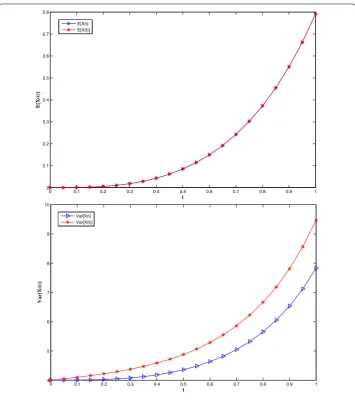
The absolute errors of the expectation and variance ofX(t) with the Euler, RK, and RK methods andh= _ ,h=_ are shown in Tables , . In Figure , the expectation and variance of the exact and numerical solutions of Example  with the RK method and

h= 

are compared.

Figures ,  show thatE[Xn] andVar[Xn] of the numerical solutions of stochastic initial value problems via random Runge-Kutta methods of the fourth order are close toE[X(t)] andVar[X(t)], respectively, ash→.

5 Applications in the electric circuits with noise Consider the following RC circuit with constant parameters:

RdQ(t)_dt +_CQ(t) =V(t) +α(t)W(t),

Q() =Q, ()

(15)

Figure 2 Expectations and variances ofX(t) andXnwith the RK4 method andh=₂₀1.

Brownian motion andα(t) is a nonrandom function that shows the inﬁrmity and intensity of noise at timet.

Now, solving this stochastic diﬀerential equation, we have

eRCt _dQ₍_t_{) +}  RCe

t

RC_Q₍_t₎_dt₌  Re

t

RC_V₍_t₎_dt₊  Rα(t)e

t

RC_dB₍_t_). _()

Now, by assumingg(t,x) =eRCt _x_{and using Theorem , we conclude}

deRCt _Q₍_t₎ ₌  RCe

t

RC_Q₍_t₎_dt₊_eRCt _dQ₍_t_). _()

By () and () we have

Q(t) =eRC–t

Q+



R

t



eRCs _V₍_s₎_ds₊  R

t



α(s)eRCs _dB₍_s₎

(16)

Now, we computeQnfrom the random fourth order Runge-Kutta method,

and by setting

(17)

Table 5 Absolute error of the expectation and variance ofQnwithh=₂₀1

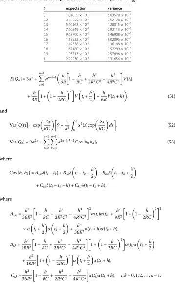
t expectation variance

(18)

Figure 3 Expectations and variances ofQ(t) andQnwithh=201.

6 Conclusion

In this paper, the numerical solution of a stochastic diﬀerential equation is discussed by fourth order Runge-Kutta methods in detail. The results can be compared with [, ]. Our comparison showed that this method has more accuracy than the Euler method and the second order Runge-Kutta methods in [, ].

Competing interests

The authors declare that they have no competing interests.

Authors’ contributions

All authors contributed equally to the writing of this paper. All authors read and approved the ﬁnal manuscript.

Author details

1_{Department of Mathematics, College of Basic Sciences, Karaj Branch, Islamic Azad University, Alborz, Iran.}2_Department

of Mathematics, Naragh Branch, Islamic Azad University, Naragh, Iran.

Acknowledgements

(19)

Received: 22 June 2014 Accepted: 30 January 2015

References

1. Cortés, JC, Jódar, L, Villafuerte, L: Numerical solution of random diﬀerential equations: a mean square approach. Math. Comput. Model.45, 757-765 (2007)

2. Khodabin, M, Maleknejad, K, Rostami, M, Nouri, M: Numerical solution of stochastic diﬀerential equations by second order Runge-Kutta methods. Math. Comput. Model.53, 1910-1920 (2011)

3. Khodabin, M, Maleknejad, K, Rostami, M, Nouri, M: Interpolation solution in generalized stochastic exponential population growth model. Appl. Math. Model.36, 1023-1033 (2012)

4. Soboleva, TK, Pleasants, AB: Population growth as a nonlinear stochastic process. Math. Comput. Model.38, 1437-1442 (2003)

5. Koskodan, R, Allen, E: Construction of consistent discrete and continuous stochastic models for multiple assets with application to option valuation. Math. Comput. Model.48, 1775-1786 (2008)

6. Cortés, JC, Jódar, L, Villafuerte, L: Random linear-quadratic mathematical models: computing explicit solutions and applications. Math. Comput. Simul.79, 2076-2090 (2009)

7. Kloeden, PE, Platen, E: Numerical Solution of Stochastic Diﬀerential Equations. Applications of Mathematics. Springer, Berlin (1999)

8. Milstein, GN: Numerical Integration of Stochastic Diﬀerential Equations. Kluwer Academic, Dordrecht (1995) 9. Calbo, G, Cortés, JC, Jódar, L: Random analytic solution of coupled diﬀerential models with uncertain initial condition

and source term. Comput. Math. Appl.56, 785-798 (2008)

10. Cortés, JC, Jódar, L, Camacho, F, Villafuerte, L: Random Airy type diﬀerential equations: mean square exact and numerical solutions. Comput. Math. Appl.60, 1237-1244 (2010)

11. Cortés, JC, Jódar, L, Villafuerte, L, Company, R: Numerical solution of random diﬀerential models. Math. Comput. Model.54, 1846-1851 (2011)

12. Cortés, JC, Jódar, L, Villafuerte, L, Villanueva, RJ: Computing mean square approximations of random diﬀusion models with source term. Math. Comput. Simul.76, 44-48 (2007)

13. Maleknejad, K, Khodabin, M, Rostami, M: Numerical solution of stochastic Volterra integral equations by stochastic operational matrix based on block pulse functions. Math. Comput. Model.55, 791-800 (2012)

14. Cortés, JC, Jódar, L, Villafuerte, L: Mean square numerical solution of random diﬀerential equations: facts and possibilities. Comput. Math. Appl.53, 1098-1106 (2007)

15. Soong, TT: Random Diﬀerential Equations in Science and Engineering. Academic Press, New York (1973)

16. Calbo, G, Cortés, JC, Jódar, L, Villafuerte, L: Analytic stochastic process solutions of second-order random diﬀerential equations. Appl. Math. Lett.23, 1421-1424 (2010)

17. Oksendal, B: Stochastic Diﬀerential Equations: An Introduction with Applications, 5th edn. Springer, New York (1998) 18. Lighthill, MJ: An Introduction to Fourier Analysis and Generalised Functions. Cambridge University Press, Cambridge