R E S E A R C H
Open Access
A dynamically consistent nonstandard finite
difference scheme for a predator–prey model
Muhammad Sajjad Shabbir
1*, Qamar Din
2, Muhammad Safeer
2, Muhammad Asif Khan
2and
Khalil Ahmad
1*Correspondence:
[email protected] 1Department of Mathematics, Air
University, Islamabad, Pakistan Full list of author information is available at the end of the article
Abstract
The interaction between prey and predator is one of the most fundamental processes in ecology. Discrete-time models are frequently used for describing the dynamics of predator and prey interaction with non-overlapping generations, such that a new generation replaces the old at regular time intervals. Keeping in view the dynamical consistency for continuous models, a nonstandard finite difference scheme is proposed for a class of predator–prey systems with Holling type-III functional response. Positivity, boundedness, and persistence of solutions are investigated. Analysis of existence of equilibria and their stability is carried out. It is proved that a continuous system undergoes a Hopf bifurcation at its interior equilibrium, whereas the discrete-time version undergoes a Neimark–Sacker bifurcation at its interior fixed point. A numerical simulation is provided to strengthen our theoretical discussion.
MSC: 39A30; 40A05; 92D25; 92C50
Keywords: Predator–prey model; Nonstandard finite difference scheme; Persistence; Stability; Neimark–Sacker bifurcation
1 Introduction
Many real-life biological models including prey–predator interactions often are governed by nonlinear differential equations. For these nonlinear differential systems analytical so-lutions are not always easy to investigate. One of the most challenging tasks is solving these nonlinear differential equations efficiently. There are several methods for converting con-tinuous differential systems to their discrete counterparts. The most conventional way for this purpose is to implement standard difference methods such as Euler approxima-tions and Runge–Kutta methods. However, numerical instabilities are observed with the implementation of standard finite difference schemes. In order to get rid of these numer-ical instabilities, one can implement nonstandard finite difference schemes introduced by Mickens [1].
Generally, a nonstandard finite difference scheme is based on the set of rules aimed at preserving the most dynamical properties of the associated continuous-time model, such as boundedness, positivity of solutions, stability of steady states, conservation laws, and bifurcations. In other words, the main advantage of these nonstandard finite difference schemes is to preserve the significant properties of their continuous analogs and
quently give reliable numerical results. On the other hand, the construction of these non-standard finite difference schemes is not always a straightforward task and there are no general criteria for their construction, and these may be considered as major drawbacks for nonstandard finite difference schemes.
Predator–prey interactions belong to the most important ways that species interact in ecological communities. Predator–prey models can reasonably be seen as the building blocks for the ecosystems. Mathematical models governed by differential equations are more appropriate for the species in which populations are overlapped. In the case of non-overlapping generations, discrete-time models governed by difference equations are more suitable than differential equations. Discretization of differential equations is one way to produce discrete-time models governed by difference equations. Numerical methods are implemented to differential equations in order to produce discrete-time models for predator–prey systems. A discrete-time model is said to be dynamically consistent with its continuous counterpart if the two demonstrate a similar dynamical behavior, such as boundedness and persistence of solutions, stability behavior of steady states, chaos, and bi-furcation [2]. Forward Euler approximations and piecewise constant arguments are more frequently used methods to obtain discrete-time counterparts of predator–prey models. But both of these methods are lacking the dynamical consistency with their continuous counterparts. Ushiki [3] proposed a discrete-time predator–prey model with implementa-tion of forward Euler approximaimplementa-tion, and it was investigated that the discrete-time system undergoes period-doubling bifurcation and the route to chaos was also discussed. Jing and Yang [4] implemented an Euler forward scheme to obtain a discrete version of the prey–predator system. Furthermore, in their paper they discussed period-doubling and Neimark–Sacker bifurcations. Similarly, Liu and Xiao [5] presented complex dynamics for a discrete Lotka–Volterra system after implementation of Euler method. For a similar type of investigations related to predator–prey systems the interested reader is referred to [6–
17]. All these studies reveal that the discrete predator–prey models with implementation of Euler approximation are dynamically inconsistent with their continuous counterparts. On the other hand, some other researchers implemented piecewise constant arguments to produce a discrete analog of the predator–prey system. Jiang and Rogers [18] imple-mented piecewise constant arguments to study the competitive case, and Krawcewicz and Rogers [19] investigated the cooperative case. Recently, Din [20–22] applied piece-wise constant arguments to various classes of predator–prey system and investigated bi-furcation and chaos control for discrete models. All these investigations reveal dynamical inconsistency between the discrete-time and continuous-time systems.
Next, we consider the following Holling and Leslie type predator–prey model [36]:
where xandyrepresent prey and predator population densities, respectively. Further-more, the growth rate for prey species is considered to be logistic with intrinsic growth raterand carrying capacityk, the consumption of prey is considered to be Holling type-III functional response,βdenotes the half-saturation constant,sis the intrinsic growth rate for prey population,hrepresents the quantity of food which prey provides for the conver-sion of predator birth, andy/xdenotes the Leslie–Gower term which measures the loss in the predator population due to rarity of its favorite food. Moreover, all parametersr,k,α,
β,s,hare positive constants.
He and Lai [6] investigated stability, period-doubling bifurcation, Neimark–Sacker bi-furcation and chaos control for a discrete counterpart of (1) with application of Euler forward approximation. Consequently, their investigation reveals the dynamical inconsis-tency between the discrete-time and continuous-time system because there is no chance of flip bifurcation in system (1). Keeping in view the dynamical consistency of model (1), the following discrete-time counterpart of (1) is proposed by implementing a Mickens type nonstandard finite difference scheme:
xn+1–xn
whereδ> 0 is step size for nonstandard finite difference method. Moreover, system (2) can be transformed into the following explicit form:
xn+1=
The remaining paper is organized as follows. In Sect.2, dynamical behavior including positivity, boundededness and persistence of solutions, existence of equilibria and their stability for model (1) is carried out. In Sect.3, we prove persistence of solutions, and a stability analysis of steady states for system (3) is also discussed. Neimark–Sacker bifurca-tion is investigated in Sect.4for model (3). Finally, numerical investigations are provided in Sect.5.
2 Dynamics of system (1)
First, we discuss positivity, boundedness and permanence of solutions of system (1).
Proof Take into account system (1) with positive initial values, that is,x(0) =x0> 0 and y(0) =y0> 0. Then from system (1) with positive initial values it follows that
x(t) =x0exp positivity of solutions and the first part (prey equation) of system (1) showing thatx(t) =
x(t)(r(1 –xk(t)) –αx(t)y(t) For the investigation of steady states of system (1), the zero growth isoclines are com-puted as follows:
Then obviously one has (k, 0) as boundary equilibrium for system (1). In order to see the dynamical behavior of system (1) at (k, 0), we first compute the Jacobian matrix of system (1) at (k, 0) as follows:
Then one can easily see that (k, 0) is a saddle point. Furthermore, the components of the interior steady state (x∗,y∗) are given by
y∗=1
hx
∗,
wherex∗is a real root of the following cubic equation:
Denote= 18bcd– 4b3d+b2c2– 4c3– 27d2, whereb=αk–hkr
hr ,c=β2andd= –kβ2, then some simple calculation shows that = –4k4(hr–α)3β2+hk2r(–8hh23rr32–20hrα+α2)β4–4h3r3β6. Then
< 0 ifα<hr. Therefore, system (1) has a unique positive steady state ifα<hr. Moreover, the variational matrix at interior equilibrium (x∗,y∗) is computed as follows:
J x∗,y∗=
a small neighborhood ofs0defined by
s0=r–
2rx∗ k –
2x∗y∗αβ2
(x∗2+β2)2.
Remark2.1 There is no chance of flip bifurcation for system (1) about its positive equi-librium.
Proof According to the necessary condition for the existence of the flip bifurcation, the determinant of the Jacobian matrixJ(x∗,y∗) must be zero, that is,2rxk∗+(2xx∗∗2y+∗βαβ2)22+ x
In this section, first of all we prove that system (3) is also permanent with similar para-metric conditions to that for system (1).
Lemma 3.1 Assume thatαk2<rhβ2,then system(3)is permanent.
1+shδkyn, and again by a simple comparison argument one has
limn→∞supyn≤kh for alln≥0. Now considering again the first equation of system (3) we
Next, we see the dynamics of model (3) at its steady states. First, the variational matrix of system (3) at boundary equilibrium (k, 0) is computed as follows:
The eigenvalues ofV(k, 0) are given byλ1= 1 –1+rδrδ andλ2= 1 +sδ. Now, it is easy to observe that|λ2|> 1 and|λ1|< 1 for allr,δ> 0. Therefore, (k, 0) is a saddle point for system (3). Furthermore, the variational matrixV(x∗,y∗) of system (3) at positive steady state is computed as follows:
V x∗,y∗=
⎛ ⎝1+
2αδx∗3y∗
(x∗2+β2)2
1+δr – αδx∗2
(1+rδ)(x∗2+β2)
sδ h(1+sδ)
1 1+sδ
⎞ ⎠.
Furthermore, the characteristic polynomial ofV(x∗,y∗) is computed as follows:
P(λ) =λ2–
1 1 +rδ +
2αδx∗3y∗
(x∗2+β2)2(1 +rδ)+
1 1 +sδ
λ
+sαδ
2x∗2(x∗2+β2) +h((x∗2+β2)2+ 2αδx∗3y∗)
h(x∗2+β2)2(1 +rδ)(1 +sδ) . (7)
Moreover, due to some simple calculations, it follows from (7) that
P(1) =sδ
2(αx∗2(x∗2+β2) +h(r(x∗2+β2)2– 2αx∗3y∗))
h(x∗2+β2)2(1 +rδ)(1 +sδ) , P(–1) =sαδ
2x∗2(x∗2+β2) +h(2 +sδ)(2(x∗2+β2)2+δ(2αx∗3y∗+r(x∗2+β2)2)) h(x∗2+β2)2(1 +rδ)(1 +sδ)
> 0
(8)
and
P(0) =sαδ
2x∗2(x∗2+β2) +h((x∗2+β2)2+ 2αδx∗3y∗)
h(x∗2+β2)2(1 +rδ)(1 +sδ) .
From (8) it follows that P(1) > 0 if and only if αx∗2(x∗2 + β2) + hr(x∗2 + β2)2 –
2αhx∗3y∗> 0. Keeping in view the relationx∗=hy∗ and the existence conditionhr>α
for a unique positive equilibrium point, we have
αx∗2 x∗2+β2+hr x∗2+β22– 2αhx∗3y∗
=αx∗4+αβ2x∗2+hrx∗4+ 2hrβ2x∗2+hrβ4– 2αx∗4
= (hr–α)x∗4+β2(α+ 2hr)x∗2+hrβ4> 0.
Lemma 3.2 Assume thatα<hr,then the unique positive steady state(x∗,y∗)of system(3)
is locally asymptotically stable if the following condition holds true:
sαδ2x∗2 x∗2+β2+h x∗2+β22+ 2αδx∗3y∗<h x∗2+β22(1 +rδ)(1 +sδ).
4 Neimark–Sacker bifurcation
A Hopf (Neimark–Sacker) bifurcation is the production of a closed invariant curve from a steady state in dynamical systems with iterated maps, when the steady state (fixed point) changes stability via a pair of complex eigenvalues with unit modulus. Recently, many it-erated maps have been studied for existence and direction of Neimark–Sacker bifurcation (cf. [37–50]).
In order to study the Neimark–Sacker bifurcation in system (3) at its positive steady state (x∗,y∗), we choosesas bifurcation parameter and system (3) is described by the following a unique positive fixed point of map (12), then one has the following map with fixed point at (0, 0):
An application of Taylor expansion about (0, 0) shows that
Moreover, the characteristic polynomial for aa1121aa2212is computed as follows: is automatically satisfied. Moreover, we assume that the following condition is satisfied:
and
Then from transformation (18) it follows that
Taking into account the bifurcation theory of normal forms (cf. [51–55]) the first Lyapunov exponent at (w,z) = (0, 0) is computed as follows:
Due to the aforementioned computations, we have the following theorem.
an attracting invariant closed curve bifurcates from the equilibrium point for s>s1,and if L> 0,then a repelling invariant closed curve bifurcates from the equilibrium point for s<s1.
5 Numerical simulation and discussion
In order to dynamical consistency between (1) and (3), we taker= 1.2,k= 1.5,α= 0.45,
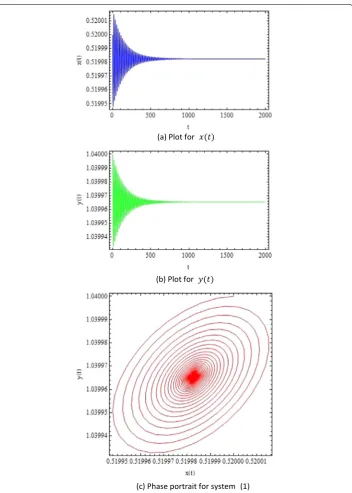
β= 0.2 andh= 0.5 for both systems (1) and (3), then both systems (1) and (3) have unique positive steady state (x∗,y∗) = (0.519983, 1.03997). Next, we takes= 0.18 for system (1),
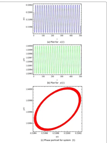
Figure 2Plots for system (1) withr= 1.2,k= 1.5,α= 0.45,β= 0.2,h= 0.5,s= 0.1659505778939415 and (x0,y0) = (0.52, 1.04)
then the equilibrium point (x∗,y∗) = (0.519983, 1.03997) is locally asymptotically stable and plots are depicted in Fig.1. Furthermore, ats0= 0.1659505778939415 system (1)
un-dergoes Hopf bifurcation at its positive steady state (x∗,y∗) = (0.519983, 1.03997) and plots are depicted in Fig.2.
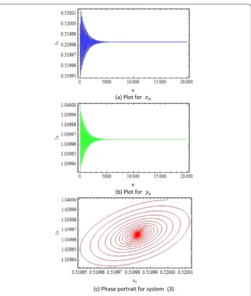
Figure 3Plots for system (3) withr= 1.2,k= 1.5,α= 0.45,β= 0.2,h= 0.5,s= 0.18,δ= 0.1 and (x0,y0) = (0.52, 1.04)
h= 0.5,δ= 0.1 ands= 0.15932296370369736 the variational matrix for model (3) is given as follows:
V(0.519983, 1.03997) =
1.01482 –0.0350006 0.0313649 0.984318
.
With some simple computation one can obtain the eigenvalues forV(0.519983, 1.03997),
λ1= 0.999567 – 0.0294149iandλ2= 0.999567 + 0.0294149isuch that|λ1,2|= 1. Moreover,
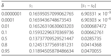
bifurcation diagrams for model (3) are given in Fig.4. On the other hand, some phase por-traits for model (3) are depicted in Fig.5. Since we have chosen exactly similar parametric values for both continuous and discrete models except the step sizeδ= 0.1 for the discrete model. In this case, the absolute difference betweens0ands1is 0.00662761. The variation
between|s0–s1|andδis given in Table1. From Table1it is obvious that for smaller step
bifurca-Figure 4Bifurcation diagrams for system (3) withr= 1.2,k= 1.5,α= 0.45,β= 0.2,h= 0.5,δ= 0.1, s∈[0.05, 0.25] and (x0,y0) = (0.52, 1.04)
tion and a Neimark–Sacker bifurcation are nearly identical, that is,|s0–s1| →0 asδ→0.
Furthermore, since system (1) is independent ofδ,s0is taken ass0= 0.1659505778939415
in Table1. Arguing as in [6], if we implement Euler forward approximation to system (1) with the aforementioned parametric values and step sizeδ= 0.1, then this discrete-time model undergoes a Neimark–Sacker bifurcation ats1= 0.17688307136658987 and thus
we have|s0–s1|= 0.0109325.
6 Concluding remarks
Figure 5Phase portraits of system (3) forr= 1.2,k= 1.5,α= 0.45,β= 0.2,h= 0.5,δ= 0.1(x0,y0) = (0.52, 1.04)
and with different values ofs
Table 1 Variation ofs1and|s1–s0|with different values ofδ
δ s1 |s1–s0|
0.0000001 0.16595057099062765 6.90331×10⁻⁹
0.0001 0.1659436748673543 6.90303×10⁻⁶
0.01 0.16526310630603203 0.000687472
0.1 0.15932296370369736 0.00662761
0.5 0.13737709529521447 0.0285735
0.8 0.12451377569181231 0.0414368
approximation. According to these investigations the discrete-time model undergoes a period-doubling bifurcation at its positive fixed point and therefore the Euler method does not seem to be bifurcation preserving.
Funding
Not applicable.
Availability of data and materials
Not applicable.
Competing interests
It is declared that none of the authors have any competing interests in this manuscript.
Authors’ contributions
All authors contributed equally to the writing of this paper. All authors read and approved the final manuscript.
Author details
1Department of Mathematics, Air University, Islamabad, Pakistan.2Department of Mathematics, University of the Poonch
Rawalakot, Azad Kashmir, Pakistan.
Publisher’s Note
Springer Nature remains neutral with regard to jurisdictional claims in published maps and institutional affiliations.
Received: 8 April 2019 Accepted: 27 August 2019 References
1. Mickens, R.: Nonstandard Finite Difference Methods of Differential Equations. World Scientific, Singapore (1994) 2. Liu, P., Elaydi, S.N.: Discrete competitive and cooperative models of Lotka–Volterra type. J. Comput. Anal. Appl.3,
53–73 (2001)
3. Ushiki, S.: Central difference scheme and chaos. Physica D4, 407–424 (1982)
4. Jing, Z., Yang, J.: Bifurcation and chaos in discrete-time predator–prey system. Chaos Solitons Fractals27, 259–277 (2006)
5. Liu, X., Xiao, D.: Complex dynamic behaviors of a discrete-time predator–prey system. Chaos Solitons Fractals32, 80–94 (2007)
6. He, Z., Lai, X.: Bifurcation and chaotic behavior of a discrete-time predator–prey system. Nonlinear Anal., Real World Appl.12, 403–417 (2011)
7. Li, B., He, Z.: Bifurcations and chaos in a two-dimensional discrete Hindmarsh–Rose model. Nonlinear Dyn.76(1), 697–715 (2014)
8. Yuan, L.-G., Yang, Q.-G.: Bifurcation, invariant curve and hybrid control in a discrete-time predator–prey system. Appl. Math. Model.39(8), 2345–2362 (2015)
9. Cheng, L., Cao, H.: Bifurcation analysis of a discrete-time ratio-dependent predator–prey model with Allee effect. Commun. Nonlinear Sci. Numer. Simul.38, 288–302 (2016)
10. Hu, D., Cao, H.: Bifurcation and chaos in a discrete-time predator–prey system of Holling and Leslie type. Commun. Nonlinear Sci. Numer. Simul.22, 702–715 (2015)
11. Jana, D.: Chaotic dynamics of a discrete predator–prey system with prey refuge. Appl. Math. Comput.224, 848–865 (2013)
12. Cui, Q., Zhang, Q., Qiu, Z., Hu, Z.: Complex dynamics of a discrete-time predator–prey system with Holling IV functional response. Chaos Solitons Fractals87, 158–171 (2016)
13. Singh, H., Dhar, J., Bhatti, H.S.: Discrete-time bifurcation behavior of a prey–predator system with generalized predator. Adv. Differ. Equ.2015, 206 (2015)
14. Ren, J., Yu, L., Siegmund, S.: Bifurcations and chaos in a discrete predator–prey model with Crowley–Martin functional response. Nonlinear Dyn.90(1), 19–41 (2017)
15. Salman, S.M., Yousef, A.M., Elsadany, A.A.: Stability, bifurcation analysis and chaos control of a discrete predator–prey system with square root functional response. Chaos Solitons Fractals93, 20–31 (2016)
16. Chen, Q., Teng, Z., Hu, Z.: Bifurcation and control for a discrete-time prey–predator model with Holling-IV functional response. Int. J. Appl. Math. Comput. Sci.23(2), 247–261 (2013)
17. Baek, H.: Complex dynamics of a discrete-time predator–prey system with Ivlev functional response. Math. Probl. Eng.
2018, 1–15 (2018)
18. Jiang, H., Rogers, T.: The discrete dynamics of symmetric competiiton in the plane. J. Math. Biol.25, 573–596 (1987) 19. Krawcewicz, W., Rogers, T.: Perfect harmony: the discrete dynamics of cooperation. J. Math. Biol.28, 383–410 (1990) 20. Din, Q.: Complexity and chaos control in a discrete-time prey–predator model. Commun. Nonlinear Sci. Numer.
Simul.49, 113–134 (2017)
21. Din, Q.: Controlling chaos in a discrete-time prey–predator model with Allee effects. Int. J. Dyn. Control6(2), 858–872 (2018)
22. Din, Q.: Stability, bifurcation analysis and chaos control for a predator–prey system. J. Vib. Control25(3), 612–626 (2019)
24. Roeger, L.-I., Allen, L.: Discrete May–Leonard competitive models I. J. Differ. Equ. Appl.10, 77–98 (2004) 25. Roeger, L.-I.: Discrete May–Leonard competitive models II. Discrete Contin. Dyn. Syst., Ser. B5(3), 841–860 (2005) 26. Roeger, L.-I.: Disctete May–Leonard competitive models III. J. Differ. Equ. Appl.10, 773–790 (2004)
27. Roeger, L.-I.: Hopf bifurcations in discrete May–Leonard competition models. Can. Appl. Math. Q.11(2), 175–194 (2003)
28. Moghadas, S.M., Alexander, M.E., Corbett, B.D.: A non-standard numerical scheme for a generalized Gause-type predator–prey model. Physica D188, 134–151 (2004)
29. Roeger, L.-I.: A nonstandard discretization method for Lotka–Volterra models that preserves periodic solutions. J. Differ. Equ. Appl.11(8), 721–733 (2005)
30. Roeger, L.-I.: Nonstandard finite-difference schemes for the Lotka–Volterra systems: generalization of Mickens’s method. J. Differ. Equ. Appl.12(9), 937–948 (2006)
31. Dimitrov, D.T., Kojouharov, H.V.: Nonstandard finite-difference methods for predator–prey models with general functional response. Math. Comput. Simul.78(1), 1–11 (2008)
32. Roeger, L.-I., Lahodny, G. Jr.: Dynamically consistent discrete Lotka–Volterra competition systems. J. Differ. Equ. Appl.
19(2), 191–200 (2013)
33. Darti, I., Suryanto, A.: Stability preserving non-standard finite difference scheme for a harvesting Leslie–Gower predator–prey model. J. Differ. Equ. Appl.21(6), 528–534 (2015)
34. Bairagi, N., Biswas, M.: A predator–prey model with Beddington–DeAngelis functional response: a non-standard finite-difference method. J. Differ. Equ. Appl.22(4), 581–593 (2016)
35. Ongun, M.Y., Ozdogan, N.: A nonstandard numerical scheme for a predator–prey model with Allee effect. J. Nonlinear Sci. Appl.10, 713–723 (2017)
36. Murray, J.D.: Mathematical Biology, 2nd edn. Springer, Berlin (1993)
37. Din, Q., Shabbir, M.S., Khan, M.A., Ahmad, K.: Bifurcation analysis and chaos control for a plant-herbivore model with weak predator functional response. J. Biol. Dyn.13(1), 481–501 (2019)
38. Abbasi, M.A., Din, Q.: Under the influence of crowding effects: stability, bifurcation and chaos control for a discrete-time predator–prey model. Int. J. Biomath.12(4), 1950044 (2019)
39. Din, Q., Hussain, M.: Controlling chaos and Neimark–Sacker bifurcation in a host-parasitoid model. Asian J. Control
21(3), 1202–1215 (2019)
40. Din, Q., Iqbal, M.A.: Bifurcation analysis and chaos control for a discrete-time enzyme model. Z. Naturforsch. A74(1), 1–14 (2019)
41. Ishaque, W., Din, Q., Taj, M., Iqbal, M.A.: Bifurcation and chaos control in a discrete-time predator-prey model with nonlinear saturated incidence rate and parasite interaction. Adv. Differ. Equ.2019, 28 (2019)
42. Elsayed, E.M., Din, Q.: Period-doubling and Neimark–Sacker bifurcations of plant-herbivore models. Adv. Differ. Equ.
2019, 271 (2019)
43. Din, Q.: A novel chaos control strategy for discrete-time Brusselator models. J. Math. Chem.56(10), 3045–3075 (2018) 44. Din, Q.: Bifurcation analysis and chaos control in discrete-time glycolysis models. J. Math. Chem.56(3), 904–931
(2018)
45. Din, Q., Donchev, T., Kolev, D.: Stability, bifurcation analysis and chaos control in chlorine dioxide–iodine–malonic acid reaction. MATCH Commun. Math. Comput. Chem.79(3), 577–606 (2018)
46. Din, Q., Saeed, U.: Bifurcation analysis and chaos control in a host-parasitoid model. Math. Methods Appl. Sci.40(14), 5391–5406 (2017)
47. Din, Q., Elsadany, A.A., Khalil, H.: Neimark–Sacker bifurcation and chaos control in a fractional-order plant-herbivore model. Discrete Dyn. Nat. Soc.2017, 6312964 (2017)
48. Din, Q.: Qualitative analysis and chaos control in a density-dependent host-parasitoid system. Int. J. Dyn. Control6(2), 778–798 (2018)
49. Din, Q.: Neimark–Sacker bifurcation and chaos control in Hassell–Varley model. J. Differ. Equ. Appl.23(4), 741–762 (2017)
50. Din, Q., Gumus, O.A., Khalil, H.: Neimark–Sacker bifurcation and chaotic behaviour of a modified host-parasitoid model. Z. Naturforsch. A72(1), 25–37 (2017)
51. Guckenheimer, J., Holmes, P.: Nonlinear Oscillations, Dynamical Systems, and Bifurcations of Vector Fields. Springer, New York (1983)
52. Robinson, C.: Dynamical Systems: Stability, Symbolic Dynamics and Chaos. CRC Press, Boca Raton (1999) 53. Wiggins, S.: Introduction to Applied Nonlinear Dynamical Systems and Chaos. Springer, New York (2003) 54. Wan, Y.H.: Computation of the stability condition for the Hopf bifurcation of diffeomorphism onR2. SIAM J. Appl.
Math.34, 167–175 (1978)
![Figure 4 Bifurcation diagrams for system (3) with r = 1.2, k = 1.5, α = 0.45, β = 0.2, h = 0.5, δ = 0.1,s ∈ [0.05,0.25] and (x0,y0) = (0.52,1.04)](https://thumb-us.123doks.com/thumbv2/123dok_us/925478.1112232/14.595.121.479.78.421/figure-bifurcation-diagrams-r-k-a-b-d.webp)