R E S E A R C H
Open Access
Modeling and energy consumption evaluation
of a stochastic wireless sensor network
Yuhong Zhang
1*and Wei Li
2Abstract
In this article, we consider a stochastic model of wireless sensor networks (WSNs) in which each sensor node randomly and alternatively stays in an active mode or a sleep mode. The active mode consists of two phases, called the full-active phase and the semi-active phase. When a referenced sensor node is in the full-active phase of the active mode, it may sense data packets, transmit the sensed packets, receive packets, and relay the received packets. However, when the phase of the sensor node switches from the full active phase to the semi-active phase, it is only able to transmit/relay data. When the referenced sensor node is in a sleep mode, it does not interact with the external world. In this article, first, we develop a stochastic model for the sensor node of a WSN, and then we derive an explicit expression of the stationary distribution of the number of data packets in the sensor node. Furthermore, we figure out some important performance measures, including the sensor node’s energy consumption for transmission, the energy consumption of the sensor operations, and the average energy consumption of the sensor node in a cycle of active and sleep modes. Also, a numerical analysis is provided to validate the proposed model and the results obtained. The novel aspects of our research are the development of a stochastic model for WSN with active and sleep features and the development of important analytical formulae for evaluating the energy consumption of a WSN. These results are expected to be useful as significant contributions to the fundamental theory of the design of various WSNs with active and sleep mode considerations.
Keywords:Energy consumption, Transmission energy consumption, Operation energy consumption, Wireless sensor networks, Stochastic model
Introduction
Wireless sensor networks (WSNs) are composed of a large number of sensors equipped with limited power and radio communication capabilities. Sensors can be deployed in extremely hostile environments, such as battlefield target areas, earthquake disaster areas, and inaccessible areas inside a chemical plant or a nuclear reactor to measure environmental changes or acquire other needed information. Such sensors are usually bat-tery operated, and it is important that they have an acceptable lifetime to accomplish the intended objec-tives. Hence, energy consumption is a crucial issue, which means that it is important to optimize (i.e., minimize) power usage [1]. There are two major techni-ques for maximizing the lifetime of the sensor network,
i.e., (1) the use of energy efficient routing and (2) the introduction of sleep/active modes for sensors [2]. A good survey of energy-efficient area monitoring for sensor networks was given in an earlier article [3]. The authors have observed that the best method for conserv-ing energy is to turn off as many sensors as possible, while still keeping the system functioning. Most applica-tions for WSNs involve battery-powered nodes with lim-ited energy, and it may not be convenient to recharge or replace the batteries. When a node exhausts its energy, it can no longer sense or relay data. Thus, most of the current research on sensor networks focuses on protocols with energy-efficient mechanisms [4-6].
Another feature of WSNs is their uncertainty, which cannot be ignored when energy issues are addressed. The major uncertainties of WSNs result primarily from (1) uncertain environmental conditions inside the sensor and (2) uncertain environmental conditions outside the sensor. The former includes the uncertainty of time in * Correspondence:[email protected]
1
Department of Engineering Technology, Texas Southern University, Houston, TX, USA
Full list of author information is available at the end of the article
each of the power modes, the uncertainty of actual lifetime, the uncertainty of the number of transitions between different power modes, the uncertainty of the sensing process, the uncertainty of the transmitting and receiving processes, and the uncertainty of packet delay. The latter includes the uncertainty of the number of sensors in the area to be covered, the uncertainty of relaying requests from neighboring sensors, the tainty of routing to the head or the gateway, the uncer-tainty of their topologies, and many other related uncertainties. Therefore, the investigation of energy-efficient WSNs and their uncertainties is a crucial issue because it offers promise for future developmental improvements in WSNs. Once a system has been designed, additional energy savings can be achieved by using dynamic power management, which shuts down the sensor node if no events occur. Every component in a node can be in different states, e.g., each sensor can be in active, idle, or sleep mode. Mathematically speaking, each sensor will have a finite number of different sta-tuses and the state space of each status also is different. The sensor node stays in each status for a random time and then transfers into another status where it stays for another random duration. A very special case occurs when each sensor only has two different statuses, e.g., active and sleep, similar as those in [7-9]. The sensor node alternatively stays in active or sleep status for a probability distributed duration. In this article, we are going to start this investigation by concentrating on the development of energy consumption in a stochastic WSN and expect our research to improve existing WSN devel-opment significantly in both theory and applications.
The rest of this article is organized as follows. “The model description” section gives the description of the modeling, and“Performance characteristics”section con-centrates on the investigation of the major performance characteristics of WSNs. And in another section, numer-ical analysis is provided, and the conclusions and recom-mendations for future research are stated in last section.
The model description
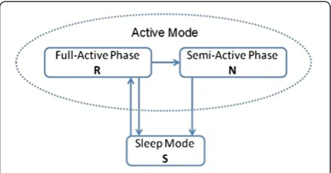
We considered a WSN in which each sensor node may alternatively stay in two major modes, i.e., active and sleep modes. The active mode consists of two phases, one of which is called the full-active phase (denoted by phase R) and the other phase is called the semi-active phase (denoted by phaseN). Sometimes we refer to the sleep mode as phaseS. Figure 1 provides a brief descrip-tion the transidescrip-tion reladescrip-tionship between these phases. From Figure 1, we know that a sensor can switch from the full-active phase to the sleep mode or to the semi-active phase. It can also change from the semi-semi-active phase to the sleep mode or from the sleep mode to the full-active phase.
In order to better describe the proposed model, the following assumptions and notations are introduced for the sensor node being investigated in this sensor network.
(a) The duration of a sensor in a sleep mode is distributed exponentially with a mean of 1/β. When a sensor is in the sleep mode, it disconnects from the external world. After the sleep duration, the sensor ends its sleep phase and returns to the full-active phase.
(b) The duration that a sensor spends in the full-active phase is a random time that has an exponential distribution with a mean of 1/α. During this period, the sensor node may:
(1) generate packets according to a Poisson process at a rate ofλ;
(2) relay packets coming from other sensors in accordance to a Poisson process at a rate of
λE; and
(3) process (transmit or relay) data packets with random exponential time with a mean of 1/μ.
(c) After the period spent in the full-active phase, the sensor node may change to either the semi-active phase or the sleep mode. The former requires there be at least one dada packet waiting to be processed, and the latter occurs when there are no data packets waiting for processing. In the semi-active phase, the sensor node may only process (transmit or relay) data packets with random exponential time with a mean of 1/μ, and it cannot generate or receive any data that are relayed from other sensors. After processing all data packets in the semi-active phase, the senor node will move to the sleep mode automatically.
(d) Each node has sufficient space, or a buffer with infinite size, to store the data it generated or forwarded from other nodes for relaying purposes.
Power consumption models of the radio in embedded devices must take both transceiver and start-up power consumption into account, and there must be an accur-ate model of the amplifier. In general, the energy con-sumed per bit transmitted is given [4,10] in terms of the energy per bit required by the electronic components of the transmitter (including the cost of startup energy), the electronic components of the receiver, the energy consumption of the transmitting amplifier to send one bit over one unit distance, and the path loss factor. In this article, we consider the energy consumption in terms of number of packets transmitted, the sensor mode status, and the switches from one mode to another. We will use the following notations:
etr: the transmitter power consumption per data packet in phaseRof the active mode;
etn: the transmitter power consumption per data packet in phaseNof the active mode;
eor: the operation power consumption per unit time in phaseRof the active mode;
eon: the operation power consumption per unit time in phaseNof the active mode;
eos: the operation power consumption per unit time in the sleep mode;
ern:the power consumption when the sensor switches from phaseRof the active mode to phaseNof the active mode;
ers: the power consumption when the sensor switches from phaseRof the active mode to the sleep mode; and
ens: the power consumption when the sensor switches from phaseNof the active mode to the sleep mode; and
esr: the power consumption when the sensor switches from the sleep mode to phaseRof the active mode.
Performance characteristics
In this section, we derive the distribution of the number of data packets in the sensor node and then develop the explicit expression of the sensor’s import-ant performance measures, including measures of the sensor’s energy consumption, the energy consumption required for operation when the sensor starts from a dif-ferent mode, the average energy consumption of a sensor in a cycle of full-active mode, semi-active mode, and sleep mode.
Distribution of the number of data packets in the sensor node
In this subsection, we derive the formula of the steady-state probability of the node when there are i (i≥0) packets (including the one being processed and
the others that are waiting) in the sensor node. Here, we denote
P(Ri) as the steady-state probability of the node when there arei(i≥0) data packets in the referenced sensor node, which is in phaseRof the active mode;
P(Ni) as the steady-state probability of the node when there areidata packets in the referenced sensor node, which is in phaseNof the active mode; and
P(S) as the steady-state probability of the node when the node is in the sleep mode.
Our major contribution to this section is the following explicit result.
Proof: In order to attain the desired result, we had to introduce three stochastic processes. One is the phase status of the node at time t, named I(t). The space of this process consists of the full-active phase (phase R),
the semi-active phase (phase N), and the sleep mode
(phaseS). The second stochastic process is the number of data packets when the sensor is in the full-active phase of the active mode at time t, called XI(t). The
space of this process is from 0 to infinity. The third sto-chastic process is the number of data packets when the sensor is in the semi-active phase of the active mode at time t, called YI(t). The space of this process is also
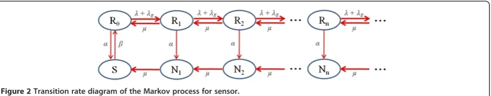
from 0 to infinity. Based on the description of the sensor node proposed in the previous section and by noting a similar but different consideration as in our other arti-cles [11,12], it is fairly simple to show that the joint process fXIð Þt ;YIð Þt g forms a multiple-dimensional Markov process with the transition rate diagram shown in Figure 2.
In Figure 2, the circle notation with Ri inside means
that the referenced sensor node is in phase R of the
active mode and that there are i data packets in the
referenced sensor node; the circle notation with Ni
inside means that the referenced sensor node is in phase
the referenced sensor node; the circle notation with S inside means that the referenced sensor node is in sleep mode. If we denote
A0¼ λþλE 0
then the corresponding transition rate matrix, Q,
of the constructed multi-dimensional Markov process
XIð Þt ;YIð Þt
applying the matrix analytical methods in stochastic modeling, such as in [13], we can derive the follow-ing result:
πi¼π0Ri; for i¼0; 1; 2; 3; 4; ⋯; ð3Þ
where matrix R is the minimal non-negative solution to the matrix-quadratic equations
R2A2þRA1þA0¼0; ð4Þ
andπ0is the unique positive solution of the equations
x0ðB0þRA2Þ ¼0 and x0ðIRÞ1e¼1; ð5Þ
in which e is a two-dimensional column vector with all its components of 1, i.e.,e¼ ð11Þ.
Furthermore, by using Theorem 6.4.1 in [13] to proceed with solving Equations (4) and (5), we finally obtain that
R¼ r1 r2
0 0
and π0¼Kðβ; αþμr2Þ ð6Þ
This theorem can now be verified by substituting the above two results in Equation (6) into Equation (3).
Remark: It is straightforward to verify that 0<r1<1 and 0<r2<1 ifαμ>0:
Measurement of energy consumption of the sensor node
As long as the formula of the steady-state probability is derived, it is not difficult to find various energy-consumption measures of the sensor node. Here, some results are listed to demonstrate how to utilize this for-mula to obtain the sensor node’s performance measures.
(1)The average energy consumption when the sensor node is in phase R of the active mode is denoted by ETR.Since the sensor will consumeetrmilliwatt (mW) of power for transmitting each data packet in phaseRof the active mode, and since the expected
number of data packets in phaseRisX 1
(2)The average energy consumption when the sensor node is in phase N of the active mode is denoted by ETN.Since the sensor will consumeetnmilliwatt (mW) of power to transmit each data packet in phaseNof the active mode, and since the expected number of data packets in this phase isX
1
sensor switches from phaseRto phaseSonly if there are not any data packets awaiting for processing. Since the sensor consumes ers milliwatt (mW) of power each time it switches from the phaseR to phaseS, we have the expression for ERS as
ERS ¼P Rð Þ0 αers¼Kαβers: ð9Þ
(4)The average energy consumed per unit time switching from the full-active phase to the semi-active phase is denoted by ERN. Since the sensor will consumeernmilliwatt (mW) of power each time the sensor switches from the full active phase of the active mode to the semi-active phase, and since the expected number of switching times from active mode to sleep mode per unit time is
X1
(5)The average energy consumed per unit time switching from the sleep mode to phase R of active mode is denoted by ESR.Since the sensor will consumeesamilliwatt (mW) of power each time the sensor switches from the sleep mode to the full-active mode, and since the expected switching number from the sleep mode to the full-active phase per unit time isP(S)β, we will have
ESR¼P Sð Þβesr¼Kðαþμr2Þβesr: ð11Þ
Node operation metrics
Now, several major metrics of the sensor node’s oper-ation are discussed, including
(1)The average delay of a data packet in the sensor node, denoted by D. Since the sensor’s data
generating rate isλand since the rate of the sensor’s relay requests from other sensors isλE, by using Little’s law [14], we have
(2)The throughput, denoted by Tn, of a sensor node which is defined as the average number of the data packets transmitted from the sensor per unit time, then
Tn ¼
(3)The probability that the sensor node is actually in sleep mode and the probability that the sensor node
is in the active mode. If we denotePSas the probability that the sensor node is actually in sleep mode, and if we denotePAas the probability that the sensor node is in the active mode, from our Theorem 1, we have
PS¼
Remark: Based on the explicit results presented above, it is apparent that the probability that the sensor is in sleep mode is not equal toβ=ðαþβÞ, and the probability that the sensor in active mode is not equal toα=ðαþβÞ, since the sensor node has to relay all data packets in the node when the sensor’s mode switches from phaseRto
phase N. This means that the active-sleep model we
developed is not a standard stochastic renewal process.
Energy consumption for operation
In this section, we concentrate on the sensor’s average energy consumption during operation in the full-active phase, semi-active phase, and sleep mode, which is denoted byEOR,EON, andEOS, respectively.
Since the sensor node will stay in the sleep mode for an exponentially distributed random time, and since the energy consumption per unit time in sleep mode is eos, it is easy to determine that EOS¼eos=β , where 1=β is the average sleep time.
Now, we consider how to obtain the sensor’s energy
consumption during its operation in phase N
(semi-active phase) and phaseR(full-active phase).
Therefore, the average energy consumption for the duration of the operation, starting from the time when there areidata packets in the semi-active phase and ending with the time when all data packets have been processed, can be given by
EON;i¼eonE TN;i
¼ieon
μ : ð16Þ
The average energy consumption for the operation of a sensor in the phaseNis
(2)The operation energy consumption when starting from the time when there are i data packets in phase R, denoted by EOR,i.Note that, in this case, the sensor node in phaseRof active mode can sense, receive, and transmit data packets and switch to phaseNor phaseR. When the sensor switches its phase from phaseRto phaseN, the sensor node only can continuously transmit the data packets that were already in the buffer of the sensor, and it cannot sensor or receive any other data packets. Thus, the operation time in this case is not as simple as theTN,idefined in above (1). In order to determine the distribution of this operation time when there areidata packets in phaseRof the active mode, we define the state when the sensor node is in sleep status as an absorbing state and construct a new Markov process with the following transition rate diagram with absorbing state (Figure3). If we denote the operation time byTR,iwhen starting from the time when there areidata packets in phaseR, then, from the definition of the distribution of the phase type as introduced in [15], we know that the distribution function of the actual operation time is a phase-type distribution and has an expression as
FTR;ið Þ ¼x P TR;i≤x
¼1eiexpð ÞTx eT; ð18Þ
forx≥0, where MatrixTcan easily be determined from the diagram in Figure3as
T ¼ consumption during operation, when starting from the time when there areidata packets in phaseRto the time when the node reached a sleep node or phaseN, is given by
When the node is in phaseRand there areidata packets, denote the initial probability byαi, and the probability vectorα¼ α0;α1;α2;⋯;αn;⋯
. Then, the energy consumption during operation in phase R, starting from the initial probabilityαi, can be expressed as
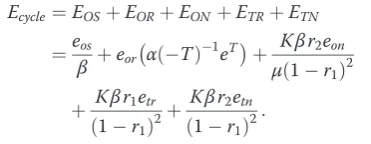
Total average energy consumption in a cycle of active sleep modes
In this section, we consider the total active average en-ergy consumption in a cycle of active and sleep modes, denoted byEcycle. Without loss of generalization, we will
ignore the switch energy consumption between sensor phases and define the cycle as the time period between the epoch when the sensor just starts its full active phase and the epoch when the sensor ends its sleep mode. In a trivial case when no data are actively processed during the cycle, the total average energy consumption is the summation of energy consumption the sensor needs to
operate when there is no any data packet in the sensor and that when the sensor is in sleep, i.e.,
Ecycle¼eor α þ
eos
β : ð21Þ
However, in the non-trivial case when at least a data packet is processed during the cycle, the energy con-sumption in this cycle should include
the energy consumption during operation in the sleep mode,EOS;
the energy consumption during operation in phaseR of the active mode,EOR;
the energy consumption during operation in phase Nof the active mode,EON;
the energy consumption for transmission in phaseR of the active mode,ETR;
the energy consumption for transmission in phaseN of the active mode,ETN.
Therefore, based on our results in “Measurement of
energy consumption of the sensor node” and “Energy
consumption for operation”sections above, we will have
Ecycle¼EOSþEORþEONþETRþETN
To verify the validity of the analytical expressions obtained in the previous section, we present the numer-ical results for a set of specific parameters in this sec-tion. The performance measures considered here are several energy consumptions, data package time delay, and the throughput.
In the model presented in this article, no limit is speci-fied for the sensor’s data storage capacity. However, in [16], we assumed that the data storage capacity of the sensor node was a finite numberC. Therefore, as a com-parison, in the following figures in this section, we treat the sensor’s data storage capacity in this model as an infinite number, i.e., C¼ 1. In addition, different per-formance measures for different Cvalues (C= 20, 10, 5) in [16] are also included in all figures. We observed and compared the effects of various performance measures in the four cases, i.e., C=1, 20, 10, and 5 versus the sensor node’s generating rate λ. We let λ change from 0.05 to 0.5. As a comparison, we used the same para-meters for this article as were used in [16], which are listed in Table 1.
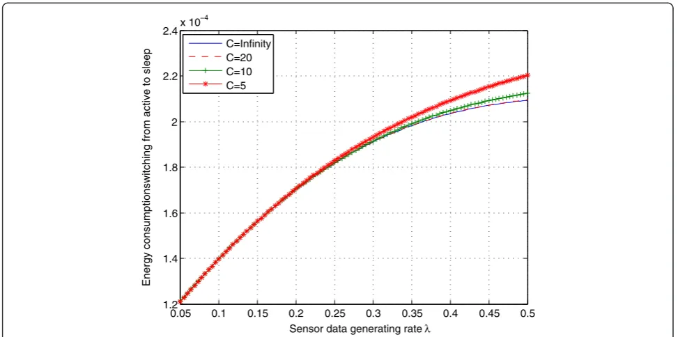
Figure 4 shows the energy consumption when the senor node switches from phaseRof the active mode to sleep mode S. It is clear that, with the increase of the sensor’s generating rate λ from 0.05 to 0.5, the switching energy assumption increases slowly. Thus, from the viewpoint of minimizing the energy consump-tion for switching from active mode to sleep mode, min-imizing the number of data packets will not have much effects. It also can be observed that the curve with
“C= 20”is much closer to the one with“C=1”than the other two curves of“C= 10”and“C= 5”. It is reasonable
to expect that the case with larger C value would be
closer to the case in whichC=1.
Figure 5 shows the energy consumption when the sen-sor node switches from sleep mode to the active mode. In this case, the energy consumption does not increase with the sensor’s generating rate, but it decreases slightly. This is because that the increased generating rate may increase the average time that the sensor stays in active mode, reduces the number of sleeps over a unit observation time and therefore reduces the energy consumption of switching from sleep mode to the active mode. In addition, similar to Figure 4, it also can be seen that the curve with “C= 20” is much closer to
the one with “C=1” than the other two curves of
“C= 10”and “C= 5”, which further verifies the validity of our formulae.
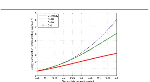
We also investigated the relationship between the change of the sensor’s generating rateλ and the average energy assumption for transmitting a package in phaseR or phase N. The curves in Figures 6 and 7 show that, with the increase of the generating rate λ, these two kinds of energy consumption will increase. This means that transmitting more data packages cause an increase in consumption. As mentioned during the discussion of the design of a WSN, the balance between energy consumption and the generation of packages is a critical issue.
The average data delay is depicted in Figure 8.
The curve with “C=1” is the delay curve for the
model in this article. It is obvious that the data delay increases when either the sensor’s generating rate λ increases or a greater number of relayed messages are being processed. Throughput of the sensor node is shown in Figure 9, and it depicts what we expected in that the throughput increases as the sensor’s generating rate increases.
Table 1 Value of parameters used in numerical analysis
λE= 0.2 μ= 0.5 β= 0.05 α= 0.1
etr= 31μw etn= 11μw err= 31μw eor= 25μw
Conclusions
In this article, we have reported the results of our study of the energy consumption of a WSN. By developing a stochastic model of the sensor node of WSNs and apply-ing the stochastic method, we derived the explicit expression of the distribution of the number of an data packets in a sensor node. Then, we determined several important performance matrices related to the sensor
node’s energy consumption. Numerical analysis was pro-vided to validate the proposed model and the results obtained. The results show that the energy consump-tion for switching between the active mode and sleep mode does not depend significantly on the number of data packets. However, the energy consumption for transmitting the data packets depends on the rate at which data packets are generated, which means that transmitting
0.05 0.1 0.15 0.2 0.25 0.3 0.35 0.4 0.45 0.5
1.2 1.4 1.6 1.8 2 2.2
2.4x 10
−4
Sensor data generating rate λ
Energy consumptionswitching from active to sleep
C=Infinity C=20 C=10 C=5
Figure 4Energy consumption for switching from the phaseRto the sleep mode.
0.05 0.1 0.15 0.2 0.25 0.3 0.35 0.4 0.45 0.5
0.0135 0.014 0.0145 0.015 0.0155 0.016 0.0165 0.017
Sensor data generating rate λ
Energy consumption switching from sleep to active
C=Infinity C=20 C=10 C=5
0.055 0.1 0.15 0.2 0.25 0.3 0.35 0.4 0.45 0.5 10
15 20 25 30
Sensor data generating rate λ
Energy consumption for transmitting in phase R
C=Infinity C=20 C=10 C=5
Figure 6Energy consumption for transmitting in the phaseNthe active mode.
0.050 0.1 0.15 0.2 0.25 0.3 0.35 0.4 0.45 0.5
1 2 3 4 5 6 7 8 9
Sensor data generating rate λ
Energy consumption for transmitting in phase N
C=Infinity C=20 C=10 C=5
0.051 0.1 0.15 0.2 0.25 0.3 0.35 0.4 0.45 0.5 1.5
2 2.5
Sensor data generating rate λ
Averge Delay of a data in the sensor
C=Infinity C=20 C=10 C=5
Figure 8Average data delay vs. sensor’s generate rate.
0.05 0.1 0.15 0.2 0.25 0.3 0.35 0.4 0.45 0.5
0.06 0.08 0.1 0.12 0.14 0.16 0.18 0.2
Sensor data generating rate λ
Throughput
C=Infinity C=20 C=10 C=5
high-density data requires the expenditure of more energy. The proposed model and analysis method are expected to be applied to the design and analysis of various WSNs, taking the times spent in active and sleep modes into consideration.
Competing interests
The authors declare that they have no competing interests.
Acknowledgments
This study was supported in part by the NSF under grant CNS-1059116 and HRD-1137732.
Author details
1Department of Engineering Technology, Texas Southern University,
Houston, TX, USA.2Department of Computer Science, Texas Southern University, Houston, TX, USA.
Received: 22 November 2011 Accepted: 24 August 2012 Published: 7 September 2012
References
1. R. Maheswar, R. Jayaparvathy, Optimal power control technique for a wireless sensor node: a new approach. Int. J. Comput. Electric. Eng.3(1), 1793–8163 (2011)
2. Z. Quan, A. Subramanian, A.H. Sayed, REACA: an efficient protocol architecture for large scale sensor networks. IEEE Trans. Wirel. Commun.6(8), 2924–2933 (2007)
3. J. Carle, D. Simplot-Ryl, Energy-efficient area monitoring for sensor networks. IEEE Comput. Mag.37(2), 40–46 (2004)
4. J. Haapola, Z. Shelby, C.A. Pomalaza-Raez, P. Mahoen,Crosslayer energy analysis of multi-hop wireless sensor networks, in Proceedings of the European Workshop on Wireless Sensor Networks(Istanbul, Turkey, 2005)
5. C.E. Jones, K.M. Sivalingam, P. Agrawal, J.C. Chen, A survey of energy efficient network protocols for wireless networks. Wirel. Netw.7(4), 343–358 (2001)
6. R. Shah, J. Rabaey,Energy aware routing for low energy ad hoc sensor networks, in Proceedings of the IEEE Wireless Communications and Networking Conference(Orlando, FL, 2002)
7. C.F. Chiasserini, M. Garetto,Modeling the performance of wireless sensor networks(Proceedings of IEEE INFOCOM’04, Hong Kong, China, 2004), pp. 9–11
8. C.F. Chiasserini, M. Garetto, An analytical model for wireless sensor networks with sleeping nodes. IEEE Trans. Mob. Comput.5(12), 1706–1718 (2006) 9. C.F. Hsin, M. Liu, Randomly duty-cycled wireless sensor networks: dynamics
of coverage? IEEE Trans. Wirel. Commun.5(11), 3182–3192 (2006) 10. S. Tang, W. Li, QoS supporting and optimal energy allocation for a cluster
based wireless sensor network. Comput. Commun.29(2569–2577) (2006) 11. W. Li, A.S. Alfa, APCSnetwork with correlated arrival process and
splitted-rate channels. IEEE J. Sel. Areas Commun.17(7), 1318–1325 (1999) 12. W. Li, Y. Fang, Performance evaluation of wireless cellular networks
with mixed channel holding times. IEEE Trans. Wirel. Commun. 7(6), 2154–2160 (2008)
13. G. Latouche, V. Ramaswami,Introduction to Matrix Analytic Methods in Stochastic Modeling, ASA-SIAM Series on Statistics and Applied Probability
(SIAM, Philadelphia, 1999)
14. P.G. Harrison, N.M. Patel,Performance Modelling of Communication Networks and Computer Architectures (Addison Wesley(Reading, MA, 1993) 15. M.F. Netuts,Matrix-Geometric Solutions in Stochastic Models (The Johns
Hopkins University Press(Baltimore, MD, 1981)
16. Y. Zhang, W. Li, An energy-based stochastic model for wireless sensor networks. Wirel. Sensor Netw3(322–328) (2011)
doi:10.1186/1687-1499-2012-282
Cite this article as:Zhang and Li:Modeling and energy consumption evaluation of a stochastic wireless sensor network.EURASIP Journal on Wireless Communications and Networking20122012:282.
Submit your manuscript to a
journal and benefi t from:
7 Convenient online submission
7 Rigorous peer review
7 Immediate publication on acceptance
7 Open access: articles freely available online
7 High visibility within the fi eld
7 Retaining the copyright to your article