Automatic scaling of F2-layer parameters from ionograms based on the
empirical orthogonal function (EOF) analysis of ionospheric electron density
Zonghua Ding1,2,3, Baiqi Ning1, Weixing Wan1, and Libo Liu1
1Institute of Geology and Geophysics, Chinese Academy of Sciences, Beijing, China 2Wuhan Institute of Physics and Mathematics, Chinese Academy of Sciences, Wuhan, China
3Graduate School of Chinese Academy of Sciences, Beijing, China
(Received April 24, 2006; Revised July 29, 2006; Accepted July 29, 2006; Online published March 15, 2007)
In this paper we apply a method based on empirical orthogonal function (EOF) analysis to automatically scale the F2-layer parameters obtained from ionograms. For a given location, the F layer’s height profiles of ionospheric electron density are represented as an EOF series with adjustable coefficients derived from the EOF analysis of electron density profiles obtained from the International Reference Ionosphere (IRI-2001) model or measured ionograms. By adjusting the coefficients of the series and combining image matching technique, we were able to construct a calculated trace that approximates as close as possible the observed ionogram F2 trace. The corresponding parameters are then known, including the critical frequency (foF2), peak height (hmF2) and maximum usable frequency [MUF(3000)F2] of the F2 layer. Polarization information is unnecessary; only an amplitude array is essential. Consequently, this method is universal and can be applied to many kinds of ionograms (even the film ionograms after an appropriate conversion of the information to the digital form from the film ionogram). To evaluate the acceptability of the obtained parameters, large numbers of foF2, hmF2 and MUF(3000)F2 values from the manually scaled ionograms at Wuhan (114.4◦E, 30.5◦N), China are compared with those from automatically scaled ionograms by the Automatic Real Time Ionogram Scaler with True height (ARTIST) and our method. The results indicate that the scaled parameters are acceptable and stable.
Key words:Ionogram, automatic scaling, electron density profile, EOF analysis.
1.
Introduction
The scaling and interpretation of ionograms are topics that are attracting continuous interest in both the scientific and practical context. Unfortunately, it is a labor-intensive and time-consuming task to manually scale ionograms and acquire the related ionospheric parameters. With the de-velopment of computer and image processing techniques, much effort has been focused on the development of tech-niques that will automatically scale ionograms (Wrightet al., 1972; Mazzetti and Perona, 1978; Reinisch and Huang, 1983; Fox and Blundell, 1989; Tsai and Berkey, 2000; Galkinet al., 2004). Most of these methods above firstly emphasize the accurate recognition of ionogram traces and then make an inversion of the density profile using iono-spheric inversion techniques (Huang and Reinisch, 1982, 2001; Titheridge, 1988). However, some complex situa-tions, such as ionogram incompleteness and external inter-ference, make ionogram automatic scaling difficult and at times even impossible.
The Automatic Real Time Ionogram Scaler with True height (ARTIST) software is the first operationally success-ful automatic scaling technique capable of robust perfor-mance (Reinisch and Huang, 1983; Reinischet al., 2005). The most widely used version to date is ARTIST4.0. A
Copyright cThe Society of Geomagnetism and Earth, Planetary and Space Sci-ences (SGEPSS); The Seismological Society of Japan; The Volcanological Society of Japan; The Geodetic Society of Japan; The Japanese Society for Planetary Sci-ences; TERRAPUB.
new release, ARTIST4.5, has been developed but it has not been adopted universally by all the users. ARTIST en-ables the autoscaling of ionogram traces by combining im-age recognition and analytical function fitting techniques. However, polarization information is required, which then expresses the electron density as a parabola or polynomials, especially as orthogonal Chebyshev polynomials with ad-justable coefficients in the F region. The coefficients of the Chebyshev polynomials are determined by fitting the calcu-lated traces obtained from the Chebyshev polynomials with the above-mentioned scaled ionogram trace. The foF2 and MUF(3000)F2 are obtained from the scaled ionogram trace, and hmF2 is acquired from the electron density profile. In addition, the contour fit method (Scotto, 2001) has been ap-plied to several standard F2 traces to match the ionogram F2 traces by the correlation technique and obtain foF2 and MUF(3000)F2.
In this paper, we present a method based on the EOF analysis of the electron density profiles. Allowing for the complications of the density profile in the E and E-F valley region, only the F-layer density profiles are represented us-ing an EOF series and that of E and E-F valley regions can be described by the universal International Reference Iono-sphere (IRI) model directly. The calculated traces from the above density profile are used to match the observed iono-gram F2 traces. From the F2 trace thus obtained and the density profiles, a number of parameters, including foF2, hmF2 and MUF(3000)F2, are obtained easily, of which the
statistical results are found to be acceptable and stable. The polarization information is thus unnecessary. The EOFs are different from the Chebyshev polynomials in being orthog-onal and experiential. By adjusting the coefficients of the EOF series, large numbers of traces are calculated and used to fit the unknown ionogram F2 trace. Thus, the ionogram F2 traces and the density profile of the F layer are obtained simultaneously, which is different from the approach using ARTIST.
2.
Analysis Procedure
2.1 Brief description of EOF analysis technique
EOF analysis is the decomposition of the dataset based on the orthogonal functions. The main idea of using EOF is to suggest a linear transformation of the original data and produce a new set of empirical orthogonal functions, which simplifies the expression of the original information. The orthogonal basic functions are naturally obtained during the calculation procedure so they involve the largest quantity of original information and moreover converge very quickly (Storch and Zwiers, 2002). The most important advantage of the EOF analysis is that only a few EOF components are required to represent most of the variability of the original dataset. The calculations of the EOFs and their coefficients are mainly based on the eigenvalue/eigenvector problems; for more details, the reader is referred to the work of Daniell
et al.(1995). EOF analysis has been used extensively in meteorology and climatology (Weare and Nasstron, 1982). Daniellet al. (1995) applied EOFs to present the altitude profiles of ion concentration in the parameterized model of the ionosphere.
2.2 Explaining the procedure of the method
It is well known that the ionogram trace and the den-sity profiles have a nearly one-to-one correspondence when there is no ledge in the F1 region. The density profile can be inversed from the scaled O wave trace. On the other hand, the observed ionogram traces can be fitted as approx-imately as possible by the calculated traces from a known density profile. If the height profile of electron density is approximated reasonably, the observed ionogram trace can be fitted satisfactorily using the calculated trace from a den-sity profile; the corresponding parameters are then obtained easily.
In the present work, the EOFs are obtained by carrying out an EOF analysis of large numbers of F-layer density profiles either inversed from the measured ionograms or di-rectly calculated from the IRI-2001 model, at Wuhan during the period of 1993–2003, which is precisely a 11-year so-lar cycle. These measured ionograms were collected by a DGS-256 Digisonde set up at Wuhan (114.4◦E, 30.6◦N), China. The height distributions of electron density are mainly influenced by the geological location, season, lo-cal time and solar and geomagnetic activity (Huanget al., 1995). It is therefore reasonable to assume that different sets of EOF analysis are made for electron density profiles under different conditions. We have simply made 64 differ-ent EOF analyses according to the four differdiffer-ent seasons, eight local time spans in each day (at 3-h intervals) and two typical solar activities (high F107:>150; low F107:<150). Some examples of the mean electron density profile and the
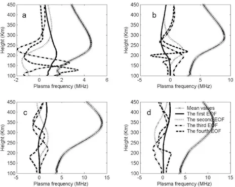
Fig. 1. The mean electron density profile and the corresponding four empirical orthogonal functions in different local times, seasons and solar activity. Panel (a) corresponds to the results at 5:00–8:00 LT, in the spring and at low solar activity. Panel (b) corresponds to those at 11:00–14:00 LT, spring and low solar activity. Panel (c) is the same as panel (b) except for high solar activity. Panel (d) is the same as panel (c) except for the different season, summer. It is obvious that the mean density profile and the corresponding four EOFs vary greatly with the different local times, seasons and solar activity.
corresponding four EOFs at different local times, seasons and solar activities are shown in Fig. 1. The electron den-sity is expressed in MegaHertz of plasma frequency in order to be compatible with figures presented later in this arti-cle. The cross, solid, dotted, dash-dotted and dashed lines represent the mean electron density and the four EOFs re-spectively. It is clear that the mean electron density profile shows the typical variation of the Chapman function, and its values are a great deal larger than those of the EOFs. The values of the different EOFs are nearly all the same. The mean electron density represents the basic character-istics, and the EOFs reflect the small variations. It is also notable that the mean electron density and the four EOFs of the different local times, seasons and solar activities are different from each other. For a more detailed discussion and analysis of the EOF analysis of electron density, the reader is referred to the articles of of Daniellet al.(1995), Wanget al.(2004) and Zhaoet al.(2005). Consequently, for a certain location, all of the F-layer density profiles can be expressed as a linear polynomial by 64 different sets of EOFs as Eq. (1).
N e(t,h)=N e(h)+
N
i=1
ai(t)∗Ei(h) (1)
Table 1. The cumulative variance of various EOFs.
and has little influence on the F2 echo trace near the foF2. The step of h is 2 km in this paper. The N denotes the rank of the adopted EOFs. The N e(h)is the time mean of the N e(t,h)distribution. The basic functionsEi(h)are the empirical orthogonal functions. The coefficient ai(t)
refers to the principal components and describes how the
N edistribution varies with time. Once the coefficientai(t)
is determined for the ionogram being processed, the F-layer density profile is known. At this point, the corresponding F2 traces and parameters can be obtained easily.
Whether the F layer represented by means of the EOF series includes both the F2 layer and the F1 layer is of no consequence to our method since the main component of this method is the scaling of the F2-layer parameters. The density profile represented by the EOF series is limited to the range of 100–450 km, from which the hmF2 is ob-tained. The calculated traces from the density profile gen-erally include the F2-layer trace, from which the foF2 and MUF3000f2 can be drawn.
Typically, the EOFs are arranged in order of decreasing variance captured in the original dataset. Table 1 lists the percentage variances of the first four EOFs. These EOFs are derived from the large number of F-layer density pro-files by the IRI-2001 model corresponding to a local time span of 11:00–14:00 LT, spring and high solar activity dur-ing 1993–2003 at Wuhan. The variance percentages of the 63 other sets of EOFs are almost the same as this one. As can be seen from Table 1, covariance contributions of the first four components are 83.148%, 15.453%, 1.221% and 0.116% respectively. Altogether, these are able to explain 99.938% of the total variance, leaving only 0.062% unex-plained. This is a clear manifestation of the important ad-vantages of the EOF analysis - EOFs converge very quickly, and only a few EOF components are required to represent most of the variability of the original dataset. Consequently, we only adopt the first four EOFs, and theNis set to 4 sim-ply.
Once the EOF analysis is made for the given station, the variablesN,N e(h), andEi(h)are determined, and theai(t)
only vary in a known range. Thus, for the known station, the F-layer electron density profile can be represented as Eq. (2).
Since the F-layer density profile of the ionogram being pro-cessed is represented reliably by Eq. (2), with the adjustable coefficients, the observed ionogram F2 traces should be fit-ted satisfactorily as the correspondingly calculafit-ted trace. If the coefficients of Eq. (2) are adjusted, large numbers of ionogram traces can be calculated. Thus, the observed iono-gram F2 trace should be fitted acceptably as one calculated
trace from the large numbers of calculated traces.
The coefficients of the EOF series vary within a known range after the EOF analysis. In the analysis of Table 1, the ranges of a1, a2, a3 and a4 are−4 to 3.5,−1.3 to 1.1,−0.3 to 0.26 and−0.05 to 0.056, respectively. The range of the coefficient for the first EOF is larger than that for the second EOF. The range of the coefficient for the third EOF is also obviously larger than that for the fourth EOF. That is to say, the range of the coefficient for the former rank EOF is larger than that for the latter rank EOF. Table 1 also shows that the covariance contributions of the four components (that is, a1*E1, a2*E2, a3*E3 and a4*E4) decrease very quickly in turn, of which the contribution of the first component is 83.148% and that of the fourth component is only 0.116%. To strengthen the importance of the former rank EOF on the EOF series, more adjustments are made to the coefficient of the former rank EOF. That is to say, the fitting possibility number for the former rank EOF is larger than that for the latter. The fitting possibility number is determined by the step of each coefficient when the range of each coefficient is known. To determine the step of coefficient for each rank EOF is a process of trial and error.
We have routinely calculated about 200,000 traces and as such have a sufficiently number to fit most of the observed ionogram F2 traces. The total number adopted should be large enough to match the observed ionograms. Generally speaking, the large the fitting number, the better the match-ing performance, but more requires more time. The above EOFs and coefficients are determined after the EOF analy-sis, and the large number of calculated traces can be known before the matching to the measured ionogram. Thus, these are all calculated and saved in a *.txt file for the conve-nience of an efficient processing beforehand. When applied in real time, these calculated traces are read from the *.txt file in order and used to match to the measured ionogram.
To search for the optimal trace from the large numbers of calculated traces, a matching criteria is needed. We know that an ionogram can be seen as a gray pixel image and rep-resented as a two-dimension arrayA(f,h). Here, f andh
are the transmitted frequency and virtual height of the re-flected echo, respectively. The f andh correspond to the
x- andy-axis in the two-dimensional coordinate. TheA de-notes the amplitude of the reflected echo in frequency f and virtual heighth. The array A(f,h)of the observed iono-gram are usually adjusted with a resolution of 0.1 MHz on thex- axis and 5 km on they-axis by interpolation and ex-trapolation. It is obvious that the amplitude of pixel points in the observed ionogram echo trace is usually strong and remarkable, with the exception of the external interference. Therefore, the amplitude sum of all pixel points in the ob-served ionogram echo trace should tend towards the maxi-mum. This is just the core of our matching criteria.
In addition, the calculated traces hc(f)can be repre-sented as another array, B(f,h), and adjusted to the same
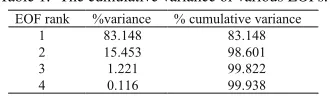
Fig. 2. Comparison of the performance of the different coefficients. The lines joining the circles and crosses denote the results from different coefficients. This ionogram is measured at Wuhan at 6:00 LT on May 2, 2001. It is clear that the calculated O and X wave traces tagged with the lines joining the circles match the observed ionogram F2 trace better than the line joining the crosses. By trying the different coefficients, the optimal coefficients are found and the calculated traces are thought to be resulting traces.
emphasize the good matching in the F2 layer, so theCvalue of pixel points in the calculated traceshc(f)near to foF2 is appointed a larger value in Eq. (3). In order to obtain optimal traces to match the observed ionogram F2 trace from large numbers of calculated traces, a correlation anal-ysis between theB(f,h)and A(f,h)is carried out. The calculated traces with maximal correlation are determined and considered to be a rough estimation of the resulting F2 traces. The corresponding coefficients are known imme-diately. Actually, the calculated O and X wave traces are simultaneously used to make the above analysis since the O wave echoes near fof2 are frequently weak or absent. We can further adjust the known coefficients of the series within the step and calculate several dozens of new traces that fluc-tuate around the roughly obtained traces. The trace that is ultimately obtained is searched from these newly calculated traces using the same matching criteria as mentioned above and generally matches the ionogram F2 trace better. This can be thought of as a refined process. This complete pro-cedure is illustrated in Fig. 2. Since the observed ionogram is always seen as a gray array, it is drawn into a gray picture in this paper.
The lines that link the circles and crosses in Fig. 2 de-note the calculated traces and the related density profiles, respectively, in terms of the EOF series from the different coefficients. It is obvious that the calculated O wave and X wave traces tagged with the line joining the circles fit the
observed ionogram F2 traces more satisfactorily. Therefore, we believe the results from the coefficients corresponding to the line joining the circles perform better than those corre-sponding to the line joining the crosses. The optimal efficients can be determined by repeatedly trying the co-efficients. The calculated traces from the optimal coeffi-cients can then be considered to nearly being the resulting F2 traces.
This method has an intrinsic advantage of universality and stability since the polarization information is not nec-essary and the information required is only a gray array. There is no need to pay much attention to the complicated situations in the observed ionogram traces, such as incom-pleteness and gaps. This method can match a complete cal-culated ionogram trace using only several weak and discon-tinuous echo signals. Because the ionogram traces in the F1 and E layer are changeable and complicated and the cal-culated traces may not sufficient to match these F1 and E traces, this method can not process the lower parts of iono-gram trace, such as the F1- and E-layer trace, very well.
Once the F2-layer traces of the observed ionogram have been fitted acceptably, some parameters, including foF2, hmF2 and MUF(3000)F2, can be obtained easily. Here, MUF(3000)F2 is obtained when the corresponding trans-mission curve is tangential with the ordinary trace in the F2 region. This transmission curve is plotted using the follow-ing equation:
fo=k fv
1
cos[arctan(1+h/sina−φ/2cosφ/2)] (4)
The fois the frequency of the wave reflected obliquely, and
the fvis the equivalent vertical frequency corresponding to
fo. The k is the correction factor, which varies from 1.0 and
1.2 and is considered to be equal to 1.1 in our calculation. Thehis the height of the reflecting layer, andφis the angle at the center of the earth subtended by the path (Pezzopane, 2004).
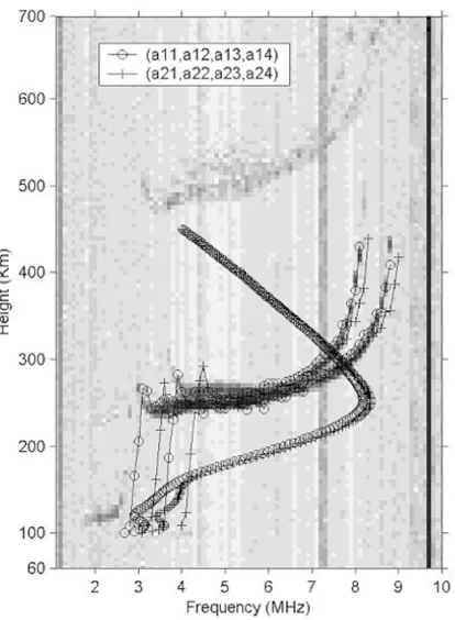
Fig. 3. The complete flowchart for a scaling of the ionogram F2 layer by our method. Panel (a) is the original ionogram observed at Wuhan at 21:30 LT on May 28, 2001. The ionogram after preprocessing is shown in panel (b). The E trace and most of the interference and noise are removed. Panel (c) is the roughly obtained traces. Panel (d) shows the final results. The lines joining the circles and crosses are the O and X wave traces in panel (c) and (d), respectively.
for reasons of simplicity. It should be clear from this figure that the automatically scaled F2 traces are nearly as good a replica of the measured ionogram F2 traces. Figure 3(d) shows the better performance of the refined processing. The final traces cover more valuable pixel points near to foF2. The automatically and manually scaled values of foF2 are 8.8 and 8.85 MHz, respectively. The corresponding hmF2 of the two cases are 383 and 388 km, respectively, while the corresponding MUF(3000)F2 values are 22.42 and 22.86 MHz, respectively. These results demonstrate the accept-ability of the autoscaling for the F2-layer parameters.
3.
Results and Discussion
3.1 Several typical samples
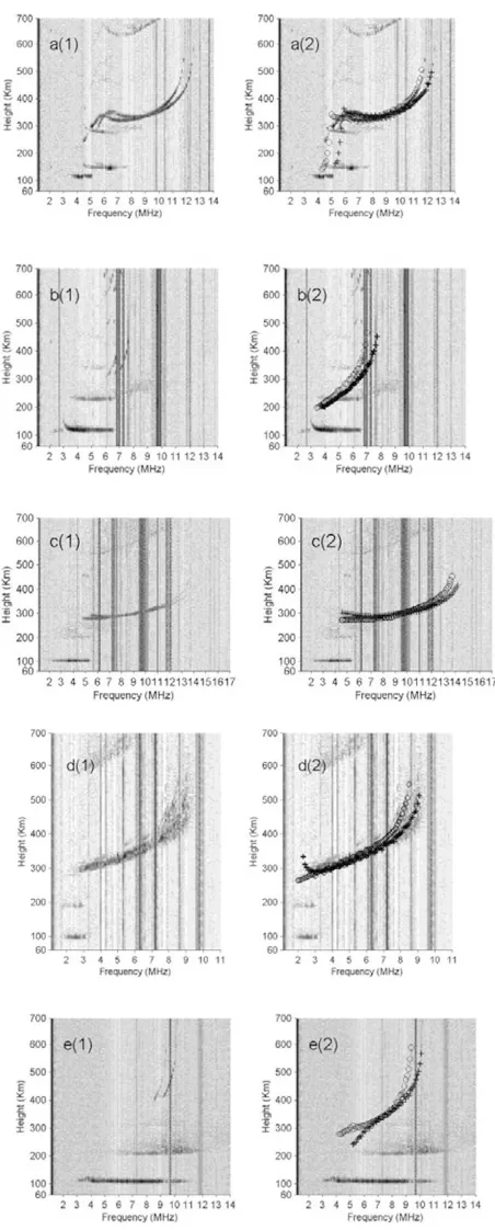
To demonstrate the features of this method qualitatively, we present five representative ionograms autoscaled in Fig. 4(a-e). These ionograms are measured by a DGS-256 Digisonde at Wuhan. Perusal of these figures will give us a good idea of the capabilities and limitations of our method. Each ionogram is plotted twice in left and right of each panel, respectively, in which the original ionogram is shown without the calculated trace, tagged with the bol “1”, and with the calculated trace, tagged with the
sym-bol “2”. The lines joining the circles and crosses denote the automatically scaled O and X traces, respectively. The F2 parameters derived from both autoscaling by our method and manually scaling are listed in Table 2 for comparison. In our work, an accurate value is considered to lie within
±0.1 MHz of the standard value for foF2,±0.5 MHz for MUF(3000)F2 and±5 km for hmF2. An acceptable value is considered to lie within±0.5 MHz of the standard value for foF2, ±2.5 MHz for MUF(3000)F2 and ±25 km for hmF2. Such limits of acceptability are in line with the URSI (International Union of Radio Science) limits of±5(is the reading accuracy).
Fig. 4. Five samples of autoscaled ionograms at Wuhan. The left and right of each panel correspond to the measured ionogram without and with the resulting traces, respectively. The ionogram traces are notable and strong, as shown in panel (a). The F1-layer and F2-layer traces are all strong. This ionogram is measured at 14:45 LT on April 30, 2001. In panel (b), the trace near foF2 of the ionogram is blurred by interference. This ionogram is measured at 07:30 LT on May 13, 2001. In panel (c), the F2 trace near to foF2 is truncated completely. This ionogram is measured at 18:00 LT on May 17, 2001. In panel (d), there is strong spread F in this ionogram, which is measured at 02:15 LT on October 16, 2001. In panel (e), the ionogram echo is very weak and strong sporadic E is also present. This ionogram is measured at 11:30 LT on October 12, 2001. Detailed explanations can be found in the text.
Table 2. The comparison of manually scaled and autoscaled F2 parameters from the five examples.
In Fig. 4(b), the F2 echo is very weak and sparse. The F2 trace near the foF2 is badly blurred and illegible due to strong interferences. This ionogram was measured at 07:30 LT on May 13, 2001. Our method satisfactorily scales the complete F2 layer trace using the several weak and discrete echoes in the F2 layer. It is also notable that the E echo is strong. The real values of foE and foF2 are 3.1 and 7.0 MHz, respectively. Although the ionization at the lower region is neglected in our EOF analysis and the difference between foE and foF2 is not very notable, the ionization at the E region does have little influence on the F2 traces obtained using our method. It is quite clear that the matched calculated traces at the lower part of F2 layer are redundant or incorrect, but the autoscaled F2 parameters are still acceptable, as shown in Table 2(b).
Figure 4(c) shows an ionogram of which the F2 trace is lost or truncated. This ionogram is measured at 18:00 LT on May 17, 2001. Our method constructs the complete F2 trace satisfactorily, which shows a strong extrapolation. The autoscaled F2 parameters are also acceptable according to Table 2(c). In Fig. 4(d), the spread F is strong and notable and the E trace is remarkable. This ionogram is measured at 02:15 LT on October 16, 2001. The scaling for the F2 layer is also acceptable.
Figure 4(e) shows how an ionogram with very weak echo traces and a strong sporadic E layer is scaled acceptably by our method. This ionogram is measured at 11:30 LT on Oc-tober 12, 2001. The F2 traces of the observed ionogram are nearly illegible, and the contour of the F2 echo trace is not well defined. Our method uses the weak echo infor-mation near fxF2 and acceptably constructs a complete F2 trace. The matched calculated F2 traces at the lower part of F2 layer are also clearly redundant and incorrect, but the autoscaled F2 parameters are acceptable.
As seen from Table 2, it is quite clear that all five of the F2 parameters from our method are completely acceptable. Consequently, we can conclude that our method is accept-able for the autoscaling of F2-layer parameters even when sporadic E, spread F, very weak echo and strong interfer-ence are present and the F2 trace near foF2 is not clearly recorded.
3.2 Statistical error analysis
Table 3. Percentages of the acceptable values of F2 parameters in the statistical analysis.
Fig. 5. The cumulative error distribution for foF2 (left), hmF2 (middle) and MUF(3000)F2 (right). The lines joining the circles, crosses and asterisks represent the results from ARTIST 4.0 and from our methods M and I, respectively.
LT, 17–20 LT and 20–23 LT) in one season and about 2000 ionograms for each season. Those ionograms in each group are selected evenly and routinely during the period of 1999– 2001.
We actually adopted two kinds of EOF in our work. We use method I and M to represent the EOFs from the electron density profiles directly calculated from the IRI model and inversed from the measured ionograms, respectively. The errorsfoF2,hmF2 andMUF(3000)F2 are calculated as the following:
foF2=foF2autoscaled−foF2manual (5.1)
hmF2=hmF2autoscaled−hmF2manual (5.2)
MUF(3000)F2=MUF(3000)F2autoscaled
−MUF(3000)F2manual (5.3)
The subscript autoscaled and manual represent the au-toscaled and the manually scaled values, respectively.
Table 3 gives the detailed acceptable percentages of all 7896 foF2, hmF2 and MUF(3000)F2 values. With respect to foF2, our method M and I has improved by 3.3% and 0.4% in acceptability compared with ARTIST 4.0, respec-tively. For hmF2, both our methods M and I are slightly superior to ARTIST 4.0 and have an increment of accept-ability of 4.8% and 0.9%, respectively. For MUF(3000)F2, the increment of acceptability of our method M is 0.8%. The MUF(3000)F2 acceptability of method I is as high as 87.4%, even though it is a little low in comparison with that of ARTIST 4.0.
The cumulative error distributions offoF2,hmF2 and
MUF(3000)F2 are shown in Fig. 5. The lines joining
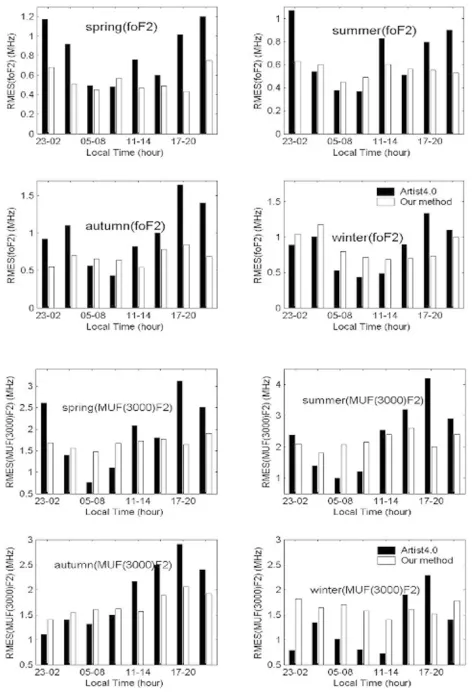
Fig. 6. The daily RMES variation of foF2 (upper) and MUF(3000)F2 (bottom). The black and white bars represent the results from ARTIST 4.0 and our method. Each black or white bar represents one RMES value during a 3-h period. For example, the bar at 23–02 LT is the result obtained during the period from 23:00 LT to 02:00 LT.
the circles, crosses and asterisks represent the results of ARTIST 4.0 and of our methods M and I, respectively. It is clear that the percentages offoF2 andhmF2 are larger than that of ARTIST 4.0 between the accurate value and the acceptable value all along, which shows the better ac-ceptability of foF2 and hmF2 from our methods. As to
pro-files of the measured ionograms more accurately than those from the method I. These results show the acceptability of both our methods for the scaling of F2-layer parameters.
The root mean square error (RMSE) represents the devi-ation from the standard values on the whole. The RMSE of foF2 is shown in Eq. (6). The subscript autoscaled and manual have the same meaning as in Eq. (5). The N de-notes the number of fof2 values calculated. The RMSE of MUF(3000)F2 is the same as in Eq. (6) with the exception of the replacement of foF2 with MUF(3000)F2.
RMSE=
We found that the RMSE variations of our method M are nearly the same as those of our method I. Consequently, we only report on the RMSE variations from method M for simplicity. The RMSE values of foF2 and MUF(3000)F2 for four seasons are given in Fig. 6. For each season, all eight RMSE values in the eight different local times are cal-culated, and eight bars are drawn. The black and white bars are the results of ARTIST 4.0 and our method, respectively. Each black or white bar represents the RMES value during the 3-h period. For example, the bars at 23–02 LT are the results obtained during the period from 23:00 LT to 02:00 LT.
The RMSE variations of ARTIST 4.0 show the obvious daily variation. The fact that the ionograms vary greatly with local time can help explain this phenomenon. How-ever, our method shows weaker variations or more stable results. It is obvious that the daily RMSE variations of both foF2 and MUF(3000)F2 from our method are slightly smoother than those of ARTIST 4.0 in all four seasons. Most of the foF2RMSE values from our method are less than those of ARTIST 4.0. The RMSE variations in both foF2 and MUF(3000)F2 from our method are usually con-sistent. When the foF2 RMSE from our method is less than that of ARTIST 4.0, the corresponding MUF(3000)F2 RMSE from our method is usually less than that of ARTIST 4.0. The scaling of the foF2 and MUF(3000)F2 parame-ters are directly related to the scaling of the F2 layer trace. Therefore, we can say that our method operates more stably and is less related to the ionograms being processed for the scaling of the F2-layer parameters.
At present, the whole autoscaling of F2-layer parameters is made using a Windows program by Matlab or C program-ming language on a common PC. The required time from the reading of the originally observed ionogram to the fi-nal output of the ionogram F2 parameters is less than 10 s. Therefore, it is possible to automatically scale F2-layer parameters of ionograms in real time.
4.
Conclusion
We introduce a method for automatically scaling F2-layer parameters from ionograms based on EOF analysis of ionospheric electron density. This method is universal and can be applied to many kinds of ionograms since it only
needs an amplitude array as input and polarization informa-tion is not necessary. The statistical results show the ac-ceptability and stability of this method for the autoscaling of F2-layer parameters. Although this method is currently not applicable to the scaling of the lower layers, such as the E and F1 layers, it has good levels of stability and accept-ability, and it does not need polarization information, which makes it a promising methodology which can be further de-veloped for the automatic scaling of whole ionogram traces.
Acknowledgments. This work was supported by National Nat-ural Science Foundation of China (40574072) and the KIP Pilot (KZCX3-SW-144) of Chinese Academy of Science.
References
Daniell, R. E., L. D. Brown, D. N. Anderson, M. W. Fox, P. H. Doherty, D. T. Decker, J. J. Sojka, and R. W. Schunk, Parameterized ionospheric model: a global ionospheric parameterization based on first principles models,Radio Sci.,30, 1499–1510, 1995.
Fox, M. W. and C. Blundell, Automatic scaling of digital ionograms,Radio Sci.,24, 747–761, 1989.
Galkin, I. A., B. W. Reinisch, G. Grinstein, G. Khmyrov, A. Kozlov, X. Q. Huang, and S. Fung, Automated exploration of the radio plasma im-ager data,J. Geophys. Res.,109, A12210, doi: 10.1029/2004JA010439, 2004.
Huang, X. Q. and B. W. Reinisch, Automatic calculation of electron den-sity profiles from digital ionograms, 2. True height inversion of top-side ionograms with the profile-fitting method,Radio Sci.,17, 837–844, 1982.
Huang, X. Q. and B. W. Reinisch, Vertical electron content from ionograms in real-time,Radio Sci.,36, 335–342, 2001.
Huang, X. Y., Y. Z. Su, and K. Zhang, Ionospheric structure and profile over Wuchang, China,Adv. Space Res.,15, 149–152, 1995.
Mather, P. M.,Computer Processing of Remotely Sensed Images: An In-troduction, 2nd Edition Wiley, Chichester, 292 pp., 1999.
Mazzetti B. and G. E. Perona, Automatic analysis of diurnal digital iono-grams,Alta Frequenza,47, 495–500, 1978 (in Italian).
Pezzopane M., Interpre: A Windows software for semiautomatic scaling of ionospheric parameters from ionograms,Computers Geosci.,30, 125– 130, 2004.
Reinisch, B. W. and X. Q. Huang, Automatic calculation of electron den-sity profiles from Digital ionograms, 3. Processing of bottomside iono-grams,Radio Sci .,18, 477–492, 1983.
Reinisch, B. W., X. Q. Huang, I. A. Galkin, V. Paznukhov, and A. Kozlov, Recent advances in real-time analysis of ionograms and ionospheric drift measurements with digisondes,J. Atmos. Solar Terr. Phys.,18, 477–492, 2005.
Scotto, C., A Method for Processing Ionograms Based on Correlation Technique,Phys. Chem. Earth.,26, 367–371, 2001.
Storch, H. V. and F. W. Zwiers,Statistical Analysis in Climate Research, Cambridge University Press, 2002.
Titheridge, J. E., The real height analysis of ionograms: a generalized formulation,Radio Sci.,23, 831–837, 1988.
Tsai, L. C. and F. T. Berkey, Ionogram analysis using fuzzy segmentation and connectedness techniques,Radio Sci.,35, 1173–1186, 2000. Wang, X., J. Shengyun, and X. Dilong, EoFs analytic representation of the
ionospheric electron density profile,Chinese Journal of Radio Science, 19(5), 560–564, 2004.
Weare, B. C. and J. S. Nasstron, Example of extended empirical orthogonal function analysis,Mon. Weather Rev.,110, 281–485, 1982.
Wright, J. W., A. R. Laird, D. Obitts, E. J. Violette, and D. McKinnis, Automatic N(h,t) profiles of the ionosphere with a digital ionosonde,
Radio Sci.,7, 1033–1043, 1972.
Zhao, B., W. Wan, L. Liu, X. Yue, and S. Venkatraman, Statistical char-acteristic of the total ion density in the topside ionosphere during the period 1996–2004 using empirical orthogonal function (EOF) analysis,
Ann. Geophys.,23, 3615–3631, 2005.